111 EAAE-IAAE Seminar ‘Small Farms: decline or persistence’ University of Kent, Canterbury, UK
26th-27th June 2009
A two-stage productivity analysis using bootstrapped Malmquist index and quantile regression
Eleni A. Kaditi and Elisavet I. Nitsi
Centre of Planning and Economic Research (KEPE) Amerikis 11, 106 72 Athens, Greece
[email protected]; [email protected]
Copyright 2009 by E. Kaditi and E. Nitsi. All rights reserved. Readers may make verbatim copies of this document for non-commercial purposes by any means, provided that this copyright notice appears on all such copies.
Abstract
This paper examines the effects of farm characteristics and government policies in enhancing productivity growth for a sample of Greek farms, using a two-stage procedure. In the 1st-stage, non-parametric estimates of Malmquist index and its decompositions are computed, while a bootstrapping procedure is applied to provide their statistical precision. In the 2nd-stage, the productivity growth estimates are regressed on various covariates using a bootstrapped quantile regression approach. The effect that the covariates exert on productivity growth of the average producer is analyzed, as well as the marginal effect of a given covariate for individuals at different points in the conditional productivity distribution. The results indicate that there exists large disparity of the covariates effect on productivity growth at different quantiles. Thus, policy suggestions should take into account the productivity distribution involved, as well as the selected policy objectives.
Keywords: Malmquist productivity index, quantile regression, bootstrap JEL codes: C14, C21, D24
A two-stage productivity analysis using bootstrapped Malmquist indices and quantile regression
Eleni A. Kaditi and Elisavet I. Nitsi
1 INTRODUCTION
The analysis of productivity and productive efficiency has received enormous attention in the literature. Productivity change and production efficiency scores are typically estimated using either a parametric or a parametric method. A well-known non-parametric mathematical linear-programming approach to frontier estimation is the Data Envelopment Analysis (DEA). This method has been developed since Charnes et al. (1978) and Färe et al. (1985), providing measures of efficiency in production based on the work of Debreu (1951) and Farell (1957), and it has been widely used due to its numerous advantages.1 The most obvious is that no particular functional form is assumed for the frontier model; whereas DEA is not subject to assumptions on the distribution errors, which might arise with parametric methods. Moreover, this approach is particularly useful in situations of multiple outputs produced from a vector of inputs, having no reliable price information that would allow estimation of stochastic frontier cost functions.
Using a two-stage procedure, the estimates of productivity change or productive efficiency obtained from such a non-parametric approach are regressed on a variety of covariates to account for exogenous factors that might affect individuals’ (or sectors’) performance, as for example in Bureau et al. (1995), Fulginiti et al. (1997), Arnade (1998), Wadud et al. (2000), Umetsu et al. (2003), Coelli and Rao (2005), and Balcombe et al. (2008). Many of these studies employ the consistent bootstrap estimation procedures proposed by Simar and Wilson (1998 and 2000) to estimate the production frontier with the best performing observations of the sample and establish statistical properties of DEA estimators. The effects of exogenous variables (e.g. producers’ size or government policies) on productivity change or efficiency are then estimated using mainly a censored or a linear model (e.g. Tobit and OLS, respectively). More recently, Simar and Wilson (2007) further proposed a double-bootstrap procedure for a truncated regression model to improve the results’ robustness.
In this literature, it is generally recognized that the resulting estimates of various effects on the conditional mean of productivity and efficiency change are not necessarily indicative of the size and nature of these effects on the tails of the productivity growth distribution. However, there has been no attempt to actually examine these. Moreover, according to Koenker and Hallock (2001), the faulty notion that is often encountered is that a form of ‘truncation on the dependent variable’, by segmenting it into subsets based on its unconditional distribution, and then doing least squares fitting on these subsets yields to consistent estimates. Such strategies are doomed to failure for all the reasons so carefully laid out in Heckman’s (1979) work on sample selection.
Quantile regression was developed by Koenker and Bassett (1978) as a robust alternative estimation technique to least squares. This study applies a two-stage analysis
1
The empirical applications of this method comprise various sectors such as agriculture, airlines, banking, electric utilities, insurance companies and public sectors.
employing a double-bootstrap technique to obtain DEA estimators and examine the issue of productivity change with a quantile regression model, in order to better understand for whom specific covariate changes are significant and how large they might be across various points of the conditional productivity distribution.
In particular, this study employs quantile regression to a sample of Greek farms to examine how farms’ productivity has been affected by government policies via regulations and subsidies, as well as through the structural evolution of the Greek agricultural sector towards larger farms. The continuous reforms of the Common Agricultural Policy (CAP) created incentives for production growth, land concentration and adoption of new technologies. However, farmers’ income continues to rely to a large extent on CAP payments. As the sector is expected to be deregulated by 2013 with the removal of such subsidies, there is currently far more pressure on farmers to be efficient. An interesting question, therefore, focuses on how farmers’ economic performance is affected by the relevant EU agricultural policies. Research by Rezitis et al. (2003) and Zhu et al. (2008) on the impact of subsidies on farms productive efficiency in Greece indicates that farmers’ performance is negatively affected by government policies. However, as is frequently the case in applied frontier research, the methods used to generate the appropriate information need to be considered.
In previous research, a stochastic frontier model and maximum-likelihood methods were applied to estimate a Cobb-Douglas or a translog production function, whereas the current analysis is the first attempt that employs a non-parametric method using data for Greece. In particular, the study employs a two-stage procedure by measuring first productivity change using a time dependent DEA method; namely the Malmquist productivity index method described in Färe et al. (1994). The statistical properties of the non-parametric estimators are determined, using a consistent bootstrap estimation procedure proposed by Simar and Wilson (1999). These estimated scores are regressed over a set of covariates, including farm characteristics and policy measures, in the framework of a quantile regression model with bootstrap. Farm-level data for the period 2001-2002 is retrieved from the Farm Accountancy Data Network (FADN) dataset. The rest of the study is organized as follows. Section 2 analyzes the Malmquist productivity index derived from the DEA method, as well as the quantile regression technique that is used for the empirical analysis. The following section gives the details of the data used, whereas Section 4 presents and discusses the empirical results. Conclusions and policy implications are included in the final section.
2 METHODOLOGY
2.1 The Malmquist Productivity Index
The Malmquist productivity index, a non-parametric DEA model under time dependent situations, is used for the estimation of productivity change. The concept of this index was introduced by Malmquist (1953), and it has been further studied and developed by several authors, as for example Caves et al. (1982) and Färe and Grosskopf (1992). It is an index evaluating total factor productivity (TFP) growth of a decision making unit (DMU – a farmer in this case), in that it reflects (i) progress or regress in efficiency along with (ii) the change in the frontier technology between two periods of time under
the multiple inputs and outputs framework. It is, therefore, defined as the product of catch-up (or recovery) and frontier-shift (or innovation) terms, respectively.
Following Cooper et al. (2007), the Malmquist index (MI) can be computed as follows:
( )
(
)
( )(
)
(
(
(( )))
)
( )(
)
( )(
)
(
(
(( )))
)
( )(
)
( )(
)
1 1 2 2 2 1 2 2 2 1 1 1 2 0 0 0 0 0 0 0 0 0 0 1 1 2 1 1 2 2 1 2 0 0 0 0 0 0 0 0 0 0 , , , , , , , , , , x y x y x y x y x y MI C F x y x y x y x y x y δ δ δ δ δ δ δ δ δ δ ⎡ ⎤ ⎡ ⎤ ⎡ ⎤ ⎢ ⎥ ⎢ ⎥ ⎢ ⎥ = × = × × = × ⎢ ⎥ ⎢ ⎥ ⎢ ⎥ ⎣ ⎦ ⎣ ⎦ ⎣ ⎦ 2 1 (1)where xo and yo indicate a vector of inputs and outputs, respectively; δi((xo, yo)i) denotes
the efficiency of (xo, yo)i with respect to period i frontier; and δj((xo, yo)i) denotes the
efficiency of (xo, yo)i with respect to period j frontier, for i=1, 2 and j=1, 2. Moreover, C
is the catch-up effect and denotes efficiency change, while F is the frontier-shift effect and denotes technology change. If MI>1, progress in the productivity of the relevant DMU has occurred from period 1 to 2, while MI=1 and MI<1 indicate respectively the status quo and deterioration in TFP.
The abovementioned scores of DMUs are measured relative to an estimated production frontier, defined as the geometrical locus of optimal production plans. In that case, the MI is based on the finite sample of observed DMUs. A bootstrap method is, therefore, used to analyze the sensitivity of the Malmquist index relative to the sampling variations of the estimated production frontier as proposed in Simar and Wilson (1999). In particular, the bivariate kernel estimator of the density of the original distance function estimates are used to preserve any temporal correlation present in the data. In this framework, an output-oriented Malmquist index is calculated with DEA based on a multi-input one-output model. Four inputs are included as follows. Capital is the value of total assets (e.g. agricultural machinery and equipment, agricultural buildings, permanent cultivation and livestock); Labor is measured as the number of hours of human labor used on individual farms during the year and includes operator, family and hired labor used on the farm; Land is the area operated measured in hectares; and Intermediates is the value of consumption of seeds, fertilizers, chemicals, feed, fuel and other miscellaneous expenses per farm.
2.2 Quantile Regression
In the quantile regression, the median is defined as the solution to the problem of minimizing a sum of absolute residuals, similarly to the sample mean used as the solution to the problem of minimizing a sum of squared residuals. The use of least squares regression leads though to biased estimates of the parameters included in the 2nd-stage of the analysis, when the data are heteroskedastic due to variable variations in the sample. Using quantile regression, the sets of slope parameters of the conditional quantile functions differ from each other as well as from the least squares slope parameters. Therefore, estimating conditional quantiles at various points of the distribution of the dependent variable allows tracing out different marginal responses of the dependent variable to changes in the covariates at these points.
The quantile regression model is defined as:
i i
i x
where yi is the MI of the ith sample farmer, i = 1,..,N, and xiis a vector of all regressors.
(
yi xiQθ
)
denotes the θth conditional quantile of yi given xi and βθ is the unknown vector of parameters to be estimated. The θth regression quantile (0<θ<1) solves the problem:(
)
⎭ ⎬ ⎫ ⎩ ⎨ ⎧ ′ − − + ′ −∑
∑
′ ≥ θ < ′θ θ β θ β θ β θ β θ β i i x i i y i iy x i i i i x y x y N Min : : 1 1 (3)Any quantile of the distribution of yi conditional on xi can be obtained by changing θ
from zero to one. This continuous change of θ relaxes the assumption of i.i.d. errors, ε, upon which the least square regression depends. Consequently, the parameter estimates are not assumed to be the same at all points on the conditional distribution.
Taking into account unobserved heterogeneity in the dependent variable of equation (2), the error term is independently but not identically distributed across individuals. The violation of this basic assumption of the standard regression model renders quantile regression to be a preferable method. In the empirical analysis, both quantile and least squares techniques are employed so as to provide a more complete picture of the conditional distribution of the dependent variable, and the partial effects the covariates exert on different quantiles.
The Malmquist index computed with DEA from the 1st-stage is then regressed using a number of covariates suggested in the literature. Starting with the variable chosen as government policies, the share of total subsidies in the total farm revenue is used, namely Subsidy. This variable may have a positive or a negative effect on productivity change. Subsidies increase productivity, if they provide to farmers an incentive to innovate or switch to new technologies, relaxing credit constraints. However, productivity may also decrease with an increase of subsidies, if farmers prefer more leisure having a higher income from subsidies.
Another farm characteristic selected is the Farm Size measured by a dummy derived from each farmer’s European Size Unit (ESU). In particular, nine different economic size classes are used based on the classification provided by FADN. It is assumed that a smaller farm may encourage its operators to adopt new technologies, though larger sized farms may be more efficient.
Two variables are included regarding the technology employed. The capital to labor ratio is used as a first proxy of farm Technology, whereas the ratio of family labor hours to total farm labor hours indicates the workforce composition. To the extent that Family Labor is more relevant in small, less competitive farms, it may be associated to a lower level of productivity.
Financial information concerning each farm is also included using two proxies. The share of Owned Land in the total land operated is expected to have a negative impact on farm’s productivity change, as long as direct costs of land rentals create stronger incentives to work the land in a more efficient manner, relative to the opportunity costs born by owned land. The availability of financial resources is proxied by a dummy variable, Loans, that equals to one when a farm has received an intermediate- or a long- term loan. This variable may reflect the ability of the farm to exploit investment opportunities and it is expected to increase productivity. A positive effect may be also
possible due to the pressure on farmers to repay their debts, and thus to limit their resource waste.
The main production activity of each farm is also indicated by a dummy variable, Specialization. It is a binary variable that equals one if a farm is mainly producing livestock and zero otherwise. This dummy is introduced to capture differences in farming practices among farms producing different types of outputs.
Farmers’ age is also likely to influence productivity, which is measured through a separate human capital variable. Age indicates the age of the farm’s operator. Younger farmers are expected to be more prone to introduce changes in farm management techniques that increase productivity, relative to elderly ones.
Moreover, a dummy that identifies whether a farm is located in a Less Favored Area (LFA) is included. Farms located in LFAs are likely to suffer from different restrictions, such as environmental constraints, low productive capacity, aged population, etc. that may reduce farms’ productivity growth.
Finally, an explicit indication of farms location is included using regional dummies. The use of regional dummies involves the assumption that farms are heterogeneous across regions. Four regions are distinguished as follows. Region 1 refers to Macedonia – Thrace; Region 2 is Ipiros – Peloponnisos – Nissoi Ioniou; Region 3 represents Thessalia, and Region 4 denotes Sterea Ellada – Nissoi Egaiou – Kriti. Binary variables that equal one or zero are, therefore, introduced, whereas Region 4 was chosen as the reference region.
In terms of the software used, the general-purpose statistical package R and FEAR (Frontier Efficiency Analysis with R) were used for the empirical analysis of this study, as standard software packages do not include procedures for non-parametric efficiency estimators, whereas only R includes procedures for statistical inference. In particular, FEAR 1.11 by Wilson (2007) and R 2.8.1 were used to compute the Malmquist index and its decompositions, as well as to implement bootstrap methods, to run the quantile regression and the appropriate hypothesis tests. Finally, the choice of bootstraps was constrained by available computer resources due to the large dataset. As indicated in the literature, 2 000 replications were performed in both stages to ensure an adequate coverage of the confidence intervals.
3 DATA AND DESCRIPTIVE STATISTICS
Data for two sequent years (2001-2002) were retrieved from the FADN dataset for Greece, which includes physical, structural, economic and financial data for about 4 000 farms. An unbalanced panel data was used to estimate the distance functions needed to construct the Malmquist productivity index, and data for 2002 were used to determine the effects of the explanatory variables. After cleaning for missing and inconsistent data, the sample size was reduced to 3 673 farms for 2001 and 3 618 for 2002. The sample used in the quantile regression includes 2 945 farms from the DEA output.
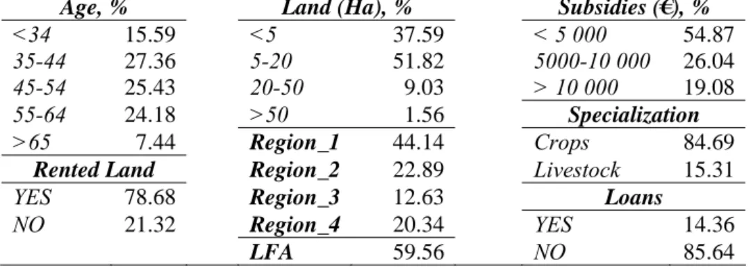
Based on this sample, a brief analysis of the agricultural sector in Greece follows. As it appears in Table 1, land operated by 51.82% of the farmers is between 5 and 20 hectares, whereas 10.59% of the producers operate in a farm that is larger than 20
hectares. Moreover, 54.87% of the sample farms receive subsidies of value lower or equal to €5 000. In terms of land ownership, about 80% of the farmers are renting land. From those, 50.69% of their total operated land is on average rented. Surprisingly, only 14.36% of the farmers reported having a long-term or an intermediate loan. As the majority of the Greek farmers are producing crops, 15.31% of the sample farms are mainly livestock producers. In addition, 57.05% of the farmers are more than 45 years old. Finally, from the 2 945 farms, 44.14% are located in Macedonia – Thrace, 22.89% in Ipiros – Peloponnisos – Nissoi Ioniou, 20.34% in Sterea Ellada – Nissoi Egaiou – Kriti and the remaining in Thessalia. Finally, almost 59.56% of the farms are located in a LFA.
Table 1 Farm Characteristics
Age, % Land (Ha), % Subsidies (€), %
<34 15.59 <5 37.59 < 5 000 54.87
35-44 27.36 5-20 51.82 5000-10 000 26.04
45-54 25.43 20-50 9.03 > 10 000 19.08
55-64 24.18 >50 1.56 Specialization
>65 7.44 Region_1 44.14 Crops 84.69
Rented Land Region_2 22.89 Livestock 15.31
YES 78.68 Region_3 12.63 Loans
NO 21.32 Region_4 20.34 YES 14.36
LFA 59.56 NO 85.64
Descriptive statistics for all variables included for the estimation of the Malmquist index are shown in Table 2. Sample farms’ average annual output totals around €20 000 in 2002. Farms employ about 3 100 labor hours per year, 82.82% of which come from family labor. Moreover, sample farms have on average 10.35 hectares of land in 2002, which was increased by 10.26% relative to 2001. Descriptive statistics for the variables used in the quantile regression are also presented in the lower part of Table 2. For instance, the average share of subsidies is about 43.28% of the farm’s revenue, whereas the average farmer’s age is 48 years for 2002.
Table 2 Descriptive Statistics
Malmquist Index output &
inputs Mean Median SD Min Max
2001 21 447 16 338 17 868 431 171 228 Production, € 2002 19 371 14 796 15 660 365 183 573 2001 29 129 22 990 24 235 221 272 553 Capital, € 2002 30 793 23 527 27 426 205 292 385 2001 3 073 2 720 1 732 177 14 300 Labor, hours 2002 3 159 2 840 1 788 144 16 240 2001 9.39 6.20 10.95 0 177.40 Land, Ha 2002 10.35 6.50 12.53 0 176.82 2001 7 999 5 956 7 211 207 95 537 Intermediates, € 2002 8 513 6 052 8 068 250 95 272
Table 2: continued
Quantile regression variables Mean Median SD Min Max
Subsidy 0.433 0.283 0.495 0 5.864 Subsidies, € 6 050 4 357 6 391 0 61 963 Technology 11.41 8.20 12.32 0.089 209.65 Family_Labor 0.828 0.903 0.197 0.112 1 Owned_Land 0.674 0.780 0.337 0 1 Age 47.87 48 12 22 84
Note: The monetary values in 2001 have been deflated using the following indices. For production: output price indices in the agricultural-livestock production (excluding subsidies); for capital: price indices of goods and services contributing to agricultural-livestock investment; and for intermediates: price indices of the consumable means of agricultural-livestock production.
4 EMPIRICAL RESULTS
4.1 The Malmquist Productivity Index
The estimated Malmquist index, its decompositions into efficiency and technology change, as well as the confidence intervals obtained from the bootstrap estimation procedure are presented in Table 3. The means for the sample farms were calculated, as well as the number of farms who experienced growth in their performance, or regress. Recall that since the MI is an output-oriented measure of productivity change, a number larger than one corresponds to improvements in performance, whereas a value less than one reflects deterioration. It appears that 44.01% of the MIs were estimated to be larger than unity; 65.37% of the farms included in the sample have an efficiency change larger than one; and only 1.56% of the farms experienced technology progress.
Table 3
Malmquist index and its decompositions
Mean Median SD Min Max
Malmquist index 1.138 0.871 0.909 0.041 4.985
Efficiency change 1.981 1.536 1.538 0.049 6.557
Technology change 0.599 0.581 0.160 0.303 1.213
Confidence intervals
Progress Regress Lower bound Upper bound
Malmquist index 1 296 1 649 1.077 1.177
Efficiency change 1 925 1 018 1.846 2.428
Technology change 46 2 899 0.421 0.635
Based on these figures, it can be further examined whether the changes in productivity, efficiency, and technology are statistically significant. The average farm of the sample appears to have a productivity growth of 13.8%, whereas the lower bound of the confidence interval is slightly greater than unity. In terms of the efficiency change component, the lower bound has again a value greater than one, which indicates that the gap between the production frontier and the relevant farms’ actual production was squeezed in the period of the present analysis. The average rate of technology change is though lower than unity indicating a downward shift of the production frontier. To sum-up, it is obvious that the observed increase in productivity growth can be explained by the increase in efficiency change for the average farm, since the change in technology lead to decreased productivity.
4.2 Quantile Regression
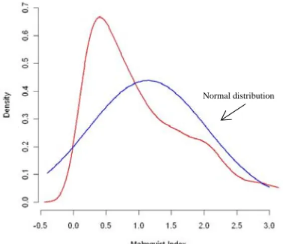
As it appears in Figure 1, the empirical distribution of productivity change is found to be highly skewed with a long right tail. The conditional median and mean fits are quite different, a fact that is partially explained by the asymmetry of the conditional density. Consequently, the median provides a more robust measure of location than the mean when distributions are skewed as with the Malmquist index.
Figure 1 Density distribution
Normal distribution
Formal testing leads to a rejection of the usual assumption of normality of the dependent variable, i.e. productivity change. The D’Agostino et al. (1990) skewness and kurtosis test is used to statistically show (at the 1% level of significance) that the dependent variable is positively skewed and kurtic (skewness = 22.173 and kurtosis = 9.644). Thus, there is a large number of farms with relatively small change in productivity, whereas farms with above average change in productivity are significantly above average. These results suggest that the distribution of the dependent variable significantly departs from normality and justifies the use of quantile regression.
Consequently, by estimating conditional quantile functions, it will be possible first to test for differences in the effects exerted on productivity change by specific covariates at various quantiles and second to take into account any possible bias due to long tails and unobserved heterogeneity among farms. The estimates of this technique are considered robust as opposed to the inefficient estimates produced by standard least squares.
In the 2nd-stage of the analysis, the effects of the various covariates on the Malmquist index were then estimated using quantile regression. The empirical results are shown in Table 4, where the 0.10, 0.25, 0.50, 0.75 and 0.90 quantiles are reported. In addition, OLS estimates showing the mean effects of all covariates are presented. The numbers in parentheses are the bootstrapped standard errors computed to improve statistical efficiency.
The quantile regression estimates are also summarized using a plot for each of the twelve covariates (and the intercept) included in the model. In Figure 2, nineteen distinct quantile regression estimates are presented for a (horizontal) quantile scale
ranging from 0.05 to 0.95 as the solid curve with filled dots. For each variable, these point estimates can be interpreted as the impact of a one-unit change of the relevant factor on productivity change holding the other variables fixed at a given specification. The shaded grey area depicts a 90 percent pointwise confidence band for the quantile regression estimates. The dotted line in each figure shows the OLS estimate of the conditional mean effect, whereas the two dashed lines represent conventional 90 percent confidence intervals for the least squares estimate.
Figure 2
OLS and Quantile regression estimates
In the first panel of the figure, the intercept of the model can be interpreted as the estimated conditional quantile function of the productivity change distribution of a farm that does not have loans, is not located in an LFA, produces mainly crops, is located in Sterea Ellada – Nissoi Egaiou – Kriti, and has the mean characteristics of the average farm (e.g. family labor is 82.8% of total labor hours, the farmer is 48 years old, etc.). That is, the explanatory variables that are not binary are chosen to reflect the means of these variables in the sample. It is worth noted that the median quantile of the distribution is farms with no change in productivity.
Each of the other plots gives information about the relevant covariate. At any chosen quantile the question that can be answered is how different is the response of productivity change from the corresponding variable, given a specification of all other conditioning factors. For the policy variable, the OLS estimate shows that productivity declines by 0.42; namely an increase of 1% of subsidies contribution to farmers’ income leads to a decrease of 0.42% in productivity. However, the quantile regression estimates show smaller changes in productivity for the lower tail of the distribution, where farms are experiencing productivity regress, and a larger change in the upper tail, where farmers are progressing. That is, a reduction in productivity by 0.12 at the 0.05 quantile up to 0.53 at the 0.95 quantile. The conventional least squares confidence interval does then a poor job of representing this range of disparity. Overall, the negative impact of subsidies on productivity change indicates that the motivation for improving productivity is lower when farmers are supported by government policies. For the farms that have experienced productivity progress, the marginal effect of subsidies is higher. This means that the farms that perform well are sensitive to subsidies and tend to progress at a lower level when receiving agricultural payments. This is a similar conclusion to the one obtained by Zhu et al. (2008).
In terms of the farm size, the variable has a positive, though relatively smaller impact on productivity change. The OLS estimates show an increase in productivity by 0.11, while the quantile regression estimates show a disparity from 0.03 at the 0.05 quantile to 0.15 at the 0.95 quantile. This implies that the larger the farm, the higher the possibility of productivity growth. This result is consistent with the conclusions of Balcombe et al. (2008). Moreover, the technology variable appears not to be statistically significant for all quantiles. Nevertheless, it may affect productivity change, as it is statistically significant for farms that regress in productivity.
Moreover, there is a negative relationship between productivity growth and farm’s workforce composition. The relevant coefficient is -0.81 for the OLS estimates and it decreases along higher quantiles (up to -1.47 at the 0.95 quantile). Its negative sign indicates that farms with a lower proportion of unpaid labor are more efficient. Family laborers appear to have fewer incentives than hired labor to act efficiently, whereas hired labor may be more qualified and more able to perform specialized tasks than family labor. This result is in accordance to Zhu et al. (2008). In addition, farms renting land may be more productive relative to farms owning the operated land; whereas the relevant coefficient is statistically significant for farms that are at the lower tail of the productivity distribution.
The variable on specialization has a positive effect on productivity, with the exception of the marginal effect in the median quantile. Interpreting the results, livestock producers are increasing their productivity relative to crop producers by 0.14 at the mean estimate, but as it is obvious from the quantile regression results, the coefficient is 0.03 in the lower quantile and significantly larger (0.57) in the upper tail of the distribution.
In terms of loans, farms’ productivity may increase if they have loans, due to the possibility of new investments. This is also justified by the fact that farmers included in the sample do not appear to be financially stressed. The coefficient representing farmers’ age suggests that older farmers might be less efficient in comparison to younger ones, though the coefficient is not statistically significant. Furthermore, the
sign of the dummy on LFAs is negative, indicating that the less favored areas are less productive relative to the other regions. Even though the estimated coefficient from the least squares is -0.12, the results obtained from the quantile regression varies from -0.03 to -0.16 along the productivity distribution.
The interpretation of the causal effects of the regional dummies, as in the corresponding least squares analysis, may be somewhat controversial. For example, it is found, that the level of productivity change is lower in all three regions in comparison to the reference region, which is Sterea Ellada – Nissoi Egaiou – Kriti. However, in the higher quantiles, that is the farms that experience the higher progress, a much larger effect appears for the three regions relative to the reference region.
Table 4
Results, Malmquist Index
OLS Quantile regression estimates
estimates 0.10 0.25 0.50 0.75 0.90 Subsidy -0.416 (0.032) *** -0.161 (0.019)*** -0.238 (0.022) *** -0.352 (0.032) *** -0.466 (0.045) *** -0.452 (0.054) *** Farm Size 0.112 (0.010) *** 0.048 (0.005) *** 0.075 (0.008) *** 0.118 (0.010) *** 0.148 (0.016) *** 0.161 (0.03) *** Technology 0.0003 (0.001) 0.0009 (0.0005) * 0.0012 (0.0007) -0.0005 (0.001) 0.0007 (0.002) -0.0016 (0.002) Family Labor -0.813 (0.086) *** -0.156 (0.051) *** -0.360 (0.071) *** -0.845 (0.134) *** -1.227 (0.174) *** -1.462 (0.229) *** Owned Land -0.011 (0.055) -0.069 (0.025) *** -0.049 (0.035) -0.065 (0.062) -0.072 (0.090) 0.230 (0.146) Loans 0.020 (0.046) 0.012 (0.028) 0.034 (0.032) 0.038 (0.055) 0.043 (0.072) 0.010 (0.108) Specialization 0.138 (0.045) *** 0.059 (0.028) ** 0.112 (0.030) *** 0.080 (0.057) 0.203 (0.093) ** 0.476 (0.152) *** Age -0.0003 (0.001) -0.0007 (0.0009) -0.0003 (0.001) -0.0006 (0.002) 0.0006 (0.002) -0.0027 (0.004) LFA -0.115 (0.034) *** -0.046 (0.019) ** -0.097 (0.024) *** -0.148 (0.034) *** -0.191 (0.062) *** -0.161 (0.087) * Region 1 -0.229 (0.045) *** -0.040 (0.023) * -0.055 (0.033) * -0.159 (0.057) *** -0.327 (0.083) *** -0.604 (0.154) *** Region 2 -0.287 (0.049) *** -0.061 (0.025) ** -0.113 (0.040) *** -0.228 (0.062) *** -0.364 (0.099) *** -0.755 (0.159) *** Region 3 -0.449 (0.059) *** -0.106 (0.031) *** -0.164 (0.039) *** -0.352 (0.067) *** -0.591 (0.102) *** -0.899 (0.157) *** Intercept 1.726 (0.132) *** 0.395 (0.076) *** 0.686 (0.097) *** 1.510 (0.171) *** 2.438 (0.244) *** 3.481 (0.398) *** Values in the parentheses are Standard Errors. Significance levels: 0.01***, 0.05**, 0.1*.
Before concluding, the importance of the differences in the quantile parameter estimates was formally examined with the relevant hypotheses testing. The corresponding test statistics for the pure location shift hypothesis and the location-scale shift hypothesis proposed by Khmaladze (1981) and Koenker and Xiao (2002) were performed. Two tests were computed for each hypothesis. A joint test that all covariates effects satisfy the null hypothesis, and a coefficient-by-coefficient version of the test. The test for the pure location shift hypothesis takes the value 44.31. The critical value for this test is 16.00, so the location shift hypothesis is decisively rejected. The critical values for the coordinatewise tests are 1.923 at 0.05, and 2.420 at 0.01, so that the effects of Subsidy,
Farm Size, Technology, Family Labor, LFA and Regions are highly significant. In terms of the location-scale shift hypothesis, it is found that the joint test statistic is now, 45.74, so that the hypothesis is rejected. Finally, for the coefficient-by-coefficient test, the covariates effects are less significant.
5 CONCLUSIONS
This study has demonstrated the use of recently developed econometric techniques for the estimation of farm-specific productivity growth, for the case of Greece. It provides a first application of a double bootstrap procedure in a two-stage estimation of a range of covariates on non-parametric estimates (DEA) of productivity growth using the method of quantile regression.
Having a distribution of productivity change that is highly skewed and kurtic, the use of the quantile regression method appears to be suitable. The importance of quantile regression estimates lies at the fact that looking at different points of the conditional distribution there is large disparity of the covariates effect on productivity growth. The empirical results indicate that government support reduces productivity growth, whereas its magnitude is almost fivefold between the lower and the upper quantile. Farm size improves farmers’ performance, while the disparity among quantiles is also fivefold. Additionally, farmers’ location plays an important role as regions appear to affect productivity differently at various points of the distribution. In particular, farmers that have significant progress, i.e. the upper quantiles, are experiencing the highest impact. Finally, farms’ specialization has a non-monotonic relationship with productivity growth among different quantiles.
Consequently, policy suggestions cannot be generalized, but should take into account the productivity distribution involved and the selected policy objectives. That is, different agricultural policies are required for farms that are observed at different points of the conditional productivity distribution, have different characteristics, and are located in different regions. In particular, possible reduction in agricultural payments may not affect farms’ performance, especially for those that experience considerable productivity progress, despite common notion. Moreover, further institutional reforms of the agricultural land market, as well as, restructuring of the overall sector towards larger farms, may contribute to the establishment of more productive farms.
Future research could proceed along two lines. First, longitudinaldata could be used in a quantile regression model to investigate how government policies and farms’ characteristic affect farms’ productivity growth over time. It would be also interesting to compare the impact of various covariates on productivity growth estimates, which are derived by a parametric and a non-parametric technique, using quantile regression.
REFERENCES
Arnade, C. (1998). Using a Programming Approach to Measure International Agricultural Efficiency and Productivity. Journal of Agricultural Economics. 49: 67-84.
Balcombe, K., S. Davidova and L. Latruffe (2008). The Use of Bootstrapped Malmquist Indices to Reassess Productivity Change Findings: An application to a sample of Polish farms. Applied Economics. 40(16): 2055-2061.
Bureau, C., R. Färe and S. Grosskopf (1995). A Comparison of Three Nonparametric Measures of Productivity Growth in European and United States Agriculture. Journal of Agricultural Economics. 46: 309-326.
Caves, D.W., L.R. Christensen and W.E. Diewert (1982). The Economic Theory of Index Numbers and the Measurement of Input, Output and Productivity. Econometrica. 50: 1393-1414.
Charnes, A., W. W. Cooper and E. Rhodes (1978). Measuring the efficiency of decision making units. European Journal of Operational Research.2: 429-444.
Coelli, T. and D.S. Prasada Rao (2005). Total Factor Productivity Growth in Agriculture: A Malmquist index analysis of 93 countries, 1980-2000. Agricultural Economics. 32(s1): 115-134.
Cooper, W.W., L.M. Seiford and K. Tone (2007). Data Envelopment Analysis: A comprehensive text with models, applications, references and DEA-solver software. Springer.
D’Agostino, R.B., A. Balanger and R.B. D’Agostino Jr. (1990). A Suggestion for Using Powerful and Informative Tests of Normality. The American Statistician. 44(4): 316-321.
Debreu, G (1951). The Coefficient of Resource Utilization. Econometrica.19: 273-292. Färe, R., S. Grosskopf, M. Norris and Z. Zhang. (1994). Productivity Growth, Technical
Progress and Efficiency Change in Industrialized Countries. American Economic Review. 84(1): 66-83.
Färe, R. and S. Grosskopf (1992). Malmquist Indexes and Fisher Indeal Indexes. The Economic Journal. 102: 158-160.
Färe, R., S. Grosskopf and C. A. K. Lovell. (1985). The Measurement of Efficiency of Production. Boston: Kluwer-Nijhoff.
Farell, M.J (1957). The measurement of productive efficiency. Journal of the Royal Statistical Society. 120(3): 253-281
.
Fulginiti, L.E. and R.K. Perrin (1997). LDC Agriculture: Nonparametric Malmquist Productivity Indices. Journal of Development Economics. 53: 373-390.
Heckman, J.J. (1979). Sample Selection Bias as a Specification Error. Econometrica. 47(1): 153-61
Khmaladze, E. V. (1981). Martingale Approach to the Theory of Goodness-of-Fit Tests. Theory of Probability and its Applications. 26: 240-257.
Koenker, R. and Z. Xiao (2002). Inference on the Quantile Regression Process. Econometrica. 70(4): 1583-1612.
Koenker, R. and K.F. Hallock (2001). Quantile Regression. Journal of Economic Perspectives. 15(4): 143-156.
Koenker, R. and G. Bassett (1978). Quantile Regression. Econometrica. 46(1): 33-50. Malmquist, S. (1953). Index Numbers and Indifference Surfaces. Trabajos de
Estadistica 4: 209-242.
Rezitis, A., K. Tsiboukas, S. Tsoukalas (2003). Investigation of Factors Influencing the Technical Efficiency of Agricultural Producers Participating in Farm Credit Programs: The case of Greece. Journal of Agricultural and Applied Economics. 35(3): 529-541.
Simar, L. and P. Wilson (2007). Estimation and Inference in Two-stage, Semi-parametric Models of Production Processes. Journal of Econometrics. 136: 31-64. Simar, L. and P. Wilson (2000). A general methodology for bootstrapping in
non-parametric frontier models. Journal of Applied Statistics. 27(6): 779-802,
Simar, L. and P. Wilson (1999). Estimating and Bootstrapping Malmquist Indices. European Journal of Operational Research 115: 459-471.
Simar, L. and P. Wilson (1998). Sensitivity analysis of efficiency scores: how to bootstrap in nonparametric frontier models. Management Science. 44: 49–61.
Umetsu, C., T. Lekprichakul and U. Chakravorty (2003). Efficiency and Technical Change in the Philippine Rice Sector: A Malmquist total factor productivity analysis. American Journal of Agricultural Economics. 85: 943-963.
Wadud, A. and B. White (2000). Farm Household Efficiency in Bangladesh: A comparison of stochastic frontier and DEA methods. Applied Economics. 32: 1665-1673.
Wilson, P.W. (2007). FEAR: A package for frontier efficiency analysis with R. Socio-Economic Planning Sciences. forthcoming.
Zhu, X., G. Karagiannis and A.O. Lansink (2008). Analysing the Impact of Direct Subsidies on the Performance of the Greek Olive Farms with a Non-monotonic Efficiency Effects Model. Paper presented in the 12th Congress of the European Association of Agricultural Economists, EAAE 2008.