A Review of \u27Big Data\u27 Variable Selection Procedures For Use in Predictive Modeling

(1)

Duquesne University

Duquesne Scholarship Collection

Electronic Theses and Dissertations

Summer 1-1-2017

A Review of 'Big Data' Variable Selection

Procedures For Use in Predictive Modeling

Sarah Papke

Follow this and additional works at:https://dsc.duq.edu/etd

This Immediate Access is brought to you for free and open access by Duquesne Scholarship Collection. It has been accepted for inclusion in Electronic Theses and Dissertations by an authorized administrator of Duquesne Scholarship Collection. For more information, please contact

[email protected].

Recommended Citation

Papke, S. (2017). A Review of 'Big Data' Variable Selection Procedures For Use in Predictive Modeling (Master's thesis, Duquesne University). Retrieved fromhttps://dsc.duq.edu/etd/182

(2)

A REVIEW OF ‘BIG DATA’ VARIABLE SELECTION PROCEDURES FOR USE IN PREDICTIVE MODELING

A Thesis

Submitted to the McAnulty College & Graduate School of Liberal Arts

Duquesne University

In partial fulfillment of the requirements for the degree of Master of Science

By Sarah Papke

(3)

Copyright by Sarah Papke

(4)

A REVIEW OF ‘BIG DATA’ VARIABLE SELECTION PROCEDURES FOR USE IN PREDICTIVE MODELING By Sarah Papke Approved May 11, 2017. Dr. Frank D’Amico Professor of Statistics (Committee Chair) Mr. Sean Tierney Professor of Statistics (Committee Member) Dr. John Kern Professor of Statistics (Department Chair) Dr. James Swindal

Dean, McAnulty College and Graduate School of Liberal Arts

(5)

ABSTRACT

A REVIEW OF ‘BIG DATA’ VARIABLE SELECTION PROCEDURES FOR USE IN PREDICTIVE MODELING

By Sarah Papke August 2017

Thesis supervised by Dr. Frank D’Amico.

Several problems arise when attempting to use traditional predictive modeling techniques on ‘big data.’ For instance, multiple linear regression models cannot be used on datasets with hundreds of variables. However several techniques are becoming common tools for selective inference as the need for analyzing big data increases. Forward selection and penalized regression models (such as LASSO, Ridge Regression, and Elastic Net) are simple modifications of multiple linear regression that can provide some guidance on simplifying a model through vari-able selection. Dimension reducing techniques, such as Partial Least Squares and Principal Components Analysis, are more complex than regression but have the ability to handle highly correlated independent variables. Each of the

(6)

afore-mentioned techniques are valuable in predictive modeling if used properly. This paper provides a mathematical introduction to these developments in selective inference. A sample dataset is used to demonstrate modeling and interpretation. Further, the applications to big data, as well as advantages and disadvantages of each procedure, are discussed.

(7)

ACKNOWLEDGEMENT

This paper would not have been possible without the help, guidance and support of several people in my life. First I’d like to thank my advisor, Dr. Frank D’Amico, for sharing his knowledge and enthusiasm throughout the research and writing process. I’d also like to thank my committee, Mr. Sean Tierney and Dr. John Kern, for giving me their time and feedback. My CMPA classmates, especially Michael McKibben, Wei Li, and Clayton Elwood, all deserve my endless gratitude: they have made the last two years truly memorable and enjoyable.

My parents, Rich and Sharon Papke, deserve the biggest thanks of all. They have always been supportive of my academic and employment pursuits, no matter how crazy or far from home they take me, and provided me with so much encouragement in my return to Pittsburgh for my Master’s degree. Last, but certainly not least, I’d like to thank my boyfriend Brian, who has been there to make me laugh and give a reality check every time I stressed too much over the last two years.

(8)

List of Figures

2.1 Hui Zou: Two-Dimensional Penalized Regression Comparison [14] 14

3.1 JMP: Variable Correlation Table 16

3.2 JMP: ANOVA table, parameter estimates, and summary statistics for

mul-tiple linear regression 17

3.3 JMP: Selection options for forward stepwise regression 19

3.4 JMP: ANOVA table, parameter estimates, and summary statistics for

stepwise regression 20

3.5 JMP: Eigenvalues for PCA 21

3.6 JMP: Eigenvectors for PCA 21

3.7 JMP: Loading Plot for PCA 22

3.8 JMP: Scree Plot for PCA 23

3.9 JMP: Principal Components Regression 24

3.10 JMP: Root Mean PRESS Plot 25

3.11 JMP: VIP Plot 27

3.12 JMP: VIP vs Coefficients Plot 28

3.13 JMP: Percent Variation Explained Plots 29

3.14 JMP: Model Coefficients for Centered and Scaled Data 30

(11)

3.16 JMP: LASSO Parameter Estimates 31

3.17 JMP: LASSO Model Summary 32

3.18 JMP: Ridge Regression Solution Path 33

3.19 JMP: Ridge Regression Parameter Estimates 33

3.20 JMP: Elastic Net Solution Path 34

3.21 JMP: Elastic Net Parameter Estimates 35

3.22 JMP: Elastic Net Model Summary 35

A.1 JMP: Distributions of Original Data 43

A.2 JMP: Distributions of Original Data 43

List of Tables

5.1 Summary of Selective Inference Techniques 41

(12)

Chapter 1:

Background and Introduction

1.1

Background

In the last 20 years, several ‘predictive modeling’ techniques have emerged to ad-dress some of the problems in analyzing ‘big data’. The phrase ‘big data’ can be traced back to John Mashey of Silicon Graphics in 1998. He said, “I was using one label for a range of issues, and I wanted the simplest, shortest phrase to convey that the boundaries of computing keep advancing.” [5] The use of big data encompasses ‘Three V’s’ (Volume, Variety, and Velocity), referring to the amount of data, types of data, and speed of data processing. [1] In 2002, the amount of information worldwide stored digitally surpassed analog information storage and by 2009, it was estimated that every US company with more than 1000 employees had at least 200 terabytes of digitally stored data. [6] The increased opportunities of learning from large datasets were accompanied by increased challenges and issues with analyzing the data cor-rectly.

There are many terms (‘machine learning,’ ‘data mining,’ ‘knowledge discovery,’ etc.) used to describe tools that sift through data, with the intention of finding pat-terns important to a question and provide answers. The aim of all these tools is the same: to make an accurate prediction. This is commonly referred to as ‘predictive modeling.’

In the paper “Statistical Learning and Selective Inference,” Jonathan Taylor and Robert Tibshirani state, “Most statistical analyses involve some kind of ‘selection’ - searching through the data for the strongest associations. Measuring the strength of the resulting associations is a challenging task, because one must account for the

(13)

effects of the selection.” [10] They go on to briefly describe several recent develop-ments for exploring these associations in data and issues with selecting variables for inclusion in the predictive model.

The objective of the thesis is to describe and compare each of the proposed mod-eling techniques discussed by Taylor and Tibshirani. Each procedure will be defined and demonstrated using an example dataset, with an explanation of common prob-lems and corrections. These same procedures will be discussed in the context of ‘big data’ analysis.

1.2

Introduction

Multiple linear regression is a common technique for predictive modeling, as the set of ˆβ coefficients effectively minimize bias, as well as being easy to interpret. In matrix form, the optimal linear regression solution is (X0X)−1_X0_y_{, where (}_X0_X₎−1 _is proportional to the covariance matrix of the predictors. [4] This inverse matrix poses a problem, however, if any of the X variables are collinear or if there are more X

variables than records in the dataset. Big datasets frequently possess one or both of these problem characteristics. Data can be pre-processed, however additional mea-sures may still be required to produce an accurate predictive model. Techniques such as Principal Components Analysis and Partial Least Squares can be employed to address the collinearity issue and provide model dimension reduction. Alternatively, penalized regression models (LASSO, ridge regression, and elastic net) can be used to shrink β parameter estimates, a useful feature when the number of variables ex-ceeds the number of records.[4] These dimension reduction and penalized regression techniques will be explored at length in the following chapters. As a reference, the following section is a list of basic definitions that will used throughout the paper.

(14)

1.3

Basic Definitions

AICc Akaike Information Criterion (corrected). A value used to compare different models for the same data, calculated by AICc = −2 ˆL+ 2k + 2k(k+1)_n₋_k₋₁ where

ˆ

L is the log likelihood, k is the number of estimated parameters, and n is the number of records in the dataset. Generally, a lower AICc indicates a better model fit.

bias The difference between a parameter’s expected value and its true value, present in penalized regression models.

BIC Bayesian Information Criterion. Like AIC (same equation, except it contains an additional term ‘log N’ in its calculation), a value used to compare different models for the same data.

big data A dataset containing, at a minimum, hundreds of records and variables.

cross-validation A process where a dataset is partitioned into k subsets, with an analysis then performedktimes. Each time the analysis is performed, a different subset is reserved for use as a validation set while the remaining sets are the training set. Thus each subset will be used in training k −1 times and in validation 1 time. After all analyses have been performed, the results of the k

analyses are averaged.

dimension reduction Transforming independent variables to a smaller dimensional space.

model complexity The number of independent variable terms present in a model.

multicollinearity Two or more X variables in a predictive model are highly corre-lated.

(15)

penalty parameter An additional term in a model to constrain the independent variable terms.

R2 _{A goodness-of-fit statistic; values range between 0 and 1, where 1 indicates that} the regression line that perfectly fits the data.

regression Determining a functional relationship between a dependent variable and one or more independent variables.

regularization Introducing a penalty parameter to a statistical model in order to prevent model overfitting.

RM SE Root Mean Square Error; A measure of a predictive model’s accuracy. selective inference Using correlations and patterns between dependent variables to

develop a predictive model.

sparse model A number of regression β coefficients are equal to 0.

standardized (normalized) data Data is put into the same scale by subtracting the mean from each element and then dividing those results by the standard deviation.

supervised learning Data has an input and a corresponding output; the dependent variable is predetermined, so analysis is ‘supervised’ at each stage by knowing (observing) the y-variable.

unsupervised learning Data has no output; input is categorized or sorted into groups and is used to study the most important contributors among the inde-pendent variables.

(16)

Chapter 2:

Statistical Procedures Useful for

Selective Inference

2.1

Multiple Linear Regression and Forward Selection

This chapter provides an overview of the mathematics behind each procedure. It is divided into three sections. The first section outlines multiple linear regression and forward stepwise regression to provide a foundation for comparison. The sec-ond section provides an explanation of the dimension reduction techniques, Principal Components Analysis and Partial Least Squares. The third section provides an ex-planation of penalized regression models, specifically LASSO, ridge regression, and elastic net. These are the recent new developments in selective inference discussed by Taylor and Tibshirani. [10]

2.1.1 Multiple Linear Regression

Traditionally, the most common technique for predictive modeling is multiple lin-ear regression using least squares. Multiple linlin-ear regression is a supervised llin-earning approach where several independent X variables are used to predict a single contin-uous dependent Y variable. The model is represented by the equation:

Y =β0+β1X1+β2X2+...+βkXk+e=β0 + n

X

i=1

βixi+e (2.1)

where Y is the outcome, βi are coefficient parameter estimates for the independent variables,Xi are the independent variables and eis random error. The linear regres-sion model [13] can be written in matrix form as y=Xβ+e, where:

(17)

y=          y1 y2 .. . yn          X=          1 x11 x12 · · · x1k 1 x21 x22 · · · x2k .. . ... ... . .. ... 1 xn1 xn2 · · · xnk          β =          β0 β1 .. . βk          e=          e1 e2 .. . en          (2.2)

The goal is to choose a model such that the sum of squared deviations between the actual outcome Y and the predicted outcome ˆY is minimized. In other words, regression finds a vector β such that :

min " _N X i=1 (yi−yˆ)2 # =min " _n X i=1 e2_i # =e0e= (2.3) (y−ˆy)0(y−yˆ) = (y−Xβ)0(y−Xβ)

where the fitted regression model is ˆy=Xβ. The minimized β vector can be found by the equation

β = (X0X)−1X0y (2.4)

The equation β = (X0X)−1_X0_y _{will appear again in a modified form in penalized}

regression models explanation of Section 2.3. The hypotheses for the multiple linear regression model are:

H0 :β1 =β2 =· · ·=βk = 0

H1 :βi 6= 0 for at least one i

2.1.2 Forward Selection

Forward selection follows the same process as multiple linear regression. Sta-tistical computing software uses an automated approach to quickly assess potential

(18)

regression models corresponding to various subsets of independent variables from a single dataset. In forward selection, independent variables are added to a regression model one at a time, usually from most significant to least significant. There are other methods (such as stepwise and backward elimination) of determining which variable enters the model next, however statistical significance is the usual default method.

After variables are ranked by significance, there are several ways to select a subset of variables to develop a model. For p-value threshold forward selection, all vari-ables added to the model have p-values below the user-defined threshold value. Any variables with p-values greater than the threshold are not included in the model. Alternatives to the p-value threshold selection are AIC and BIC. Both the AIC and BIC are based on the Likelihood function for the model. For both of these measures, a lower number indicates a better model fit; however a better model fit does not necessarily indicate a more accurate or reliable prediction.

(19)

2.2

Principal Components Analysis and Partial Least Squares

2.2.1 Principal Components Analysis

Principal Components Analysis (PCA) is an unsupervised learning process which examines the correlation between independent variables and transforms them into a set of uncorrelated component variables. [3] Although PCA removes the variation common to any two variables, it preserves the unshared variation of the individual variables. Each component can be represented by the following equation:

P Ci =wi1x1+wi2x2+· · ·+wikxk (2.5)

whereirepresents the component andwij is the weight corresponding to thejth vari-able in the corresponding component. The components are computed by eigenvalue analysis.

Begin by creating the correlation matrix of the standardized (normalized) data, then calculate the eigenvectors and corresponding eigenvalues for this matrix. (An eigenvector is a vector v such that Av = λv, where A is a square matrix and λ

is a constant multiplier called the eigenvalue. There are several linear algebra tech-niques for calculating eigenvectors and eigenvalues which will not be discussed in the context of this paper.) The eigenvectors are sorted by eigenvalue, from highest to lowest. The eigenvector with the highest eigenvalue becomes the first principal component, the eigenvector with the second highest eigenvalue becomes the second principal component, etc. Because eigenvectors corresponding to distinct eigenvalues are linearly independent, the eigenvectors and components are uncorrelated with each other. Each component explains a percentage of the variability in the X data, with the first component accounting for the most and the kth _{component explaining the}

(20)

least. One advantage of the PCA is that it can be used with datasets that have high correlation or a large number of independent variables.

If the original dataset has a dependent variable, the principal components can then be used in place of the original independent variables in a regression model, thereby reducing the number of independent variables (complexity) to a fewer num-ber. However, it is very difficult to analyze the coefficients of this model because each component depends on several of the original independent variables. The components are also developed only considering variation among the independent variables and there is no guarantee that they can be used to accurately predict Y. These issues will be further discussed at length in Chapter 4.

2.2.2 Partial Least Squares

Partial Least Squares (PLS) is a sister method to PCA that incorporates the de-pendent variable in the dimension reduction process. There are several algorithms to perform PLS regression, including methods to regress with a single dependent vari-able and methods to regress with multiple dependent varivari-ables. Similar to PCA, PLS can be used with datasets that are highly correlated or have a large number of inde-pendentX variables. PLS can also be used with datasets that have more independent variables than records or even when the dataset contains several dependent variables.

One commonly used PLS regression method is the Statistically Inspired Modifi-cation of Partial Least Squares (SIMPLS). This technique is designed for use with multiple dependent variables. However, SIMPLS can also be used to perform PLS on data with one dependent variable; in this instance, the algorithm simply terminates after one iteration and is equivalent to the Nonlinear Iterative Partial Least Squares

(21)

algorithm.

This section will focus on the Nonlinear Iterative Partial Least Squares (NIPALS) algorithm, which can be used to perform regression with a single dependent variable. This algorithm was developed in 1966 by Herman Wold for computing PCA and later modified for PLS. It is the most basic of the partial least squares algorithms and also the most computationally expensive algorithm because it iteratively performs a sequence of ordinary least squares regressions. As with PCA, the algorithm produces a set of scores and a set of loadings to use for dimension reduction.

For m independent variables and n total records composing m x n matrix X and one dependent variable y composing an n x 1 vector, the algorithm is as follows: Algorithm 1NIPALS for Partial Least Squares

1: find latent variable and principal component:

2: w=XT_y _. _{create vector}_w _{orthogonal to} _XT_y

3: w← w

kwk .convert w to a unit vector

4: t=Xw . tis a latent feature of X and y

5: p= X_tTT_tt . find principal component

6: deflate X and y:

7: X←X−tpT . residual in X unaccounted for by tpT

8: ˆc= t_tTTy_t .find regression coefficient of y as a function of t

9: y←y−tˆc . residual in y

10: repeat algorithm using deflated X and y to compute the next feature and component

11: continue to apply the algorithm until convergence

Because PLS uses the dependent variable in dimension reduction, the compo-nents derived from the algorithm are guaranteed to provide some percentage of ex-planation of the variation in Y. Moreover, PLS is a reliable method to determine high-importance variables in order to develop multiple linear regression or forward selection models.

(22)

2.3

Penalized Regression Models

Penalized regression models shrink the size of multiple linear regression coeffi-cients, thus introducing bias, while attempting to improve the prediction. The addi-tional bias attempts to correct for instances where there are more independent vari-ables than records, when varivari-ables are highly correlated, or other situations where traditional linear regression is inappropriate. This section is an overview of three types of penalized regression models: LASSO, ridge regression, and elastic net.

These three models are all modifications of multiple linear regression, each with a penalty parameter added to the (X0X)−1_{. In matrix form, this penalty parameter} appears in the form of a tuning parameter (called λ) which is added to the diagonal entries of the multiple linear regression estimation for β. The tuning parameter is algorithmically chosen by software to produce the ‘best model’, where the user can select criteria such as R2, training error, or cross-validation to give the software defi-nition of what the ‘best model’ is.

2.3.1 LASSO

The Least Absolute Shrinkage and Selection Operator (LASSO) method is a re-gression technique that performs variable selection by adding penalty,λ, to the diag-onal entries of the multiple linear regression estimation β = (X0X)−1_X0_y_{, as shown} in the equation below:

(23)

Rather than minimizing the sum of squares as multiple linear regression does, the LASSO regression minimizes the sum of squares plus the penalty parameter:

min " _N X i=1 (yi−yˆ)2+λ X j |βj| # = (2.7) min " _N X i=1 (yi−β0− X j βjxij)2+λ X j |βj| #

In standardized form, β0 = 0, so the equation can be rewritten more simply as

min " _N X i=1 (yi− X j βjxij)2+λ X j |βj| # (2.8) The term λP

j|βj| is referred to as the l1 penalty parameter. The λ (where λ ≥0) variable is a tuning parameter, which controls the magnitude of the penalty and the amount of shrinkage of theβestimates. It provides a balance between the ‘goodness of fit’ produced by the sum of squared differences and the ‘model complexity’ produced by the sum of absolute regression coefficients. [10] The λ parameter must be greater than or equal to 0. Ifλ= 0,the penalty term will not be in the model and a multiple linear regression model remains. As λ increases, the independent variables become more constrained. If ˆβo

j represents the least squares estimates, a value of λ <βˆjo will causeβcoefficients to shrink toward 0. In some instances, theβ coefficients will equal 0, effectively reducing the complexity of the model through variable selection. [11] There are many ways to select the ‘best model,’ which directly affects the value for

λ. Cross-validation is the most common method because it can be performed with any number of parameters and records.

(24)

2.3.2 Ridge Regression

Originally proposed in 1970 by Arthur E. Hoerl and Robert W. Kennard, ridge regression attempts to correct for overfitting through regularization. It takes the standard multiple linear regression estimationβ = (X0X)−1X0yand adds aλconstant parameter to the diagonal entries of theX0Xmatrix prior to inversion, providing the new estimate:

βridge = (X0X+λI)−1X0y (2.9) Ridge regression differs from the LASSO only in the penalty parameter: ridge regression uses the l2 penalty parameter, which adds the sum of squared β’s rather than the absolute value. While the l1 parameter creates a sparse model (a number of

β coefficients are equal to 0) through variable selection, thel2 parameter provides reg-ularization (l2 shrinks the coefficients but none will ever equal 0). The minimization equation looks as such:

min " _N X i=1 (yi− X j βjxij)2+λ X j β_j2 (2.10)

An important difference to note between LASSO and ridge regression is that the solution to ridge regression will bound the size of the β parameters but will never produce a β coefficient equal to 0. Similar to LASSO, cross-validation is one of the most common techniques to help select a value forλ. [12]

2.3.3 Elastic Net

Elastic Net regularization adds both the l1 and l2 penalties to the multiple linear regression model. As with both LASSO and ridge regression, λ is added to the diagonal entries of the multiple linear regression estimation β = (X0X)−1_X0_y_:

(25)

The β parameters are now predicted by finding: min " _N X i=1 (yi− X j βjxij)2+λ1 X j |βj|+λ2 X j β_j2 # (2.12)

Because Elastic Net uses both penalty parameters, the procedure allows for both the variable selection features present in the LASSO and the stability present in ridge regression. Differences between the three penalized regression models can be seen in the graph below:

Figure 2.1: Hui Zou: Two-Dimensional Penalized Regression Comparison [14]

In the figure above, the inner diamond depicts the constraint region of a two-dimensional LASSO. When the regression sum of squares is tangent to one of the

(26)

corners, the corresponding variable has been shrunk to zero. The two-dimensional depiction of the elastic net constraints is the rounded diamond (the middle shape of figure 2.1). Though the edges are curved, the region also has corners which will indi-cate that a variable has been shrunk to zero if the sum of squares is tangent to it. The outer circle in the figure is the constraint region of the ridge regression. There are no corners so no matter the constraint, all variables will still be present in the regression.

(27)

Chapter 3:

Illustrative Examples

3.1

Data Description

The dataset called Bread, from the book Discovering Partial Least Squares with JMP [2], will be used to demonstrate each of the procedures outlined in Chapter 2. This dataset contains 24 records, where each contains data regarding a variety of bread made by a commercial bakery. Each record contains 67 variables: 7 consumer attributes and 60 expert panel sensory attributes. For the purposes of this chapter, only consumer attributes will be used. The consumer attributes represent a cross-sectional study of 50 participants. Each participant rated each of the attributes from 0 to 9, with 9 being the most desirable, for each bread. The participants scores were then averaged and entered into the data as one observation. The attributes are as follows: Overall Liking, Strong Flavor, Gritty, Succulent, Full Bodied, Strong Aroma. The dataset contains no missing observations and all variables are approximately normally distributed. The independent variables have little correlation with each other, as can be seen in the correlation table in Figure 3.1:

Figure 3.1: JMP: Variable Correlation Table

It is important to note that the models in this chapter were not designed with the intention of producing the best fitting model. Rather, the model options and param-eters were kept as similar as possible in order to provide a foundation for comparison.

(28)

Also to provide consistency, all independent variables have been standardized by sub-tracting the mean of each variable and dividing by the standard deviation. All output in this chapter is produced using JMP® statistical software. [9] The full output for each analysis is provided in Appendix B.

3.2

Multiple Linear Regression and Forward Selection

3.2.1 Multiple Linear Regression

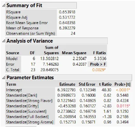
The multiple linear regression model will serve as the basis for comparison. The dependent variable is the consumer attribute Overall Liking and the independent variables are the remaining six consumer variables: Dark, Strong Flavor, Gritty, Succulent, Full Bodied, Strong Aroma. Output of multiple linear regression is as follows:

(29)

The model in figure 3.2 uses all six independent variables without selection. The F Ratio of F6,17 = 5.3536 indicates that the null hypothesis is rejected and at least one of the parameter estimates is not equal to 0. Looking at the t Ratios and p-values for the parameter estimates,Gritty is the strongest predictor in the model, while the others provide little contribution. These estimates are computed by Type III sums of squares, the most conservative type, where sums of squares are calculated for each variable as if it were the last to enter the model. Other important statistics to note are theR2Adj and the Root Mean Square Error (RMSE), as these values will be used to compare subsequent models.

3.2.2 Forward Stepwise Selection

Because many of the variables were non-significant in the multiple linear regression model, forward selection can be used to simplify the model by examining variables in order of decreasing contributions to design a subset of significant variables. Several options are available to create a model using forward selection, such as R2_, _{RM SE}_,

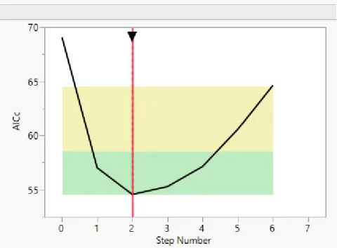
AIC, or BIC. Figure 3.3 below shows the solution path of forward selection using ‘AICc’.

(30)

Figure 3.3: JMP: Selection options for forward stepwise regression

To provide consistency with later models, the variables will be chosen by examin-ing the Akaike Information Criterion (AIC) value. AIC provides a relative indication of model quality, with lower values implying a more accurate model. The lowest AIC in the forward selection scenario occurs when only two variables,Gritty andSucculent

(31)

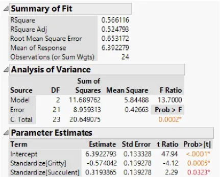
Figure 3.4: JMP: ANOVA table, parameter estimates, and summary statistics for stepwise regression

The summary statistics from the forward selection model in figure 3.4, specifi-ally r2 _{and RMSE, differ little from those in the multiple linear regression model.} Although there is no improvement in model accuracy, there is considerable improve-ment in model simplicity.

3.3

Principal Components Analysis and Partial Least Squares

3.3.1 Principal Components Analysis

Principal Components Analysis (PCA) provides an alternative to forward selection to simplify the model through dimension reduction of the independent variables. Prior to running PCA, all variables were standardized. In the output, first consider the eigenvalues and cumulative component percent, displayed in the figure below:

(32)

Figure 3.5: JMP: Eigenvalues for PCA

The percent column (calculated by dividing each eigenvalue by the total sum of all eigenvalues) indicates what portion of the variance is explained by the corresponding component. The eigenvalues represent the strength of the component; in this instance, the first three components account for nearly 75% of the total variation inX. Because the goal of PCA is dimension reduction, ideally at least 90% of the total variation could be explained by a small number of PCA variables. To see which variables contribute to each component, consider the eigenvectors:

Figure 3.6: JMP: Eigenvectors for PCA

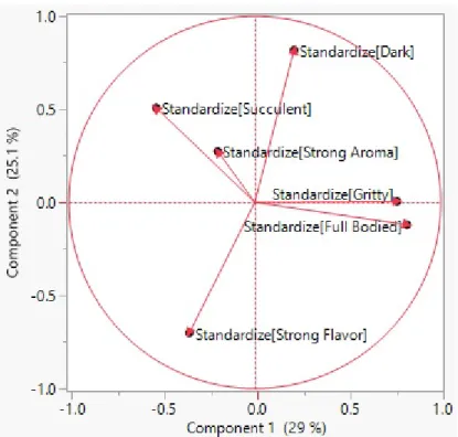
Gritty,Full Bodied, andSucculent are the strongest contributors to the first com-ponent, which is consistent with the forward selection. Similar information can be determined from the Loading Plot, which plots the first principal component eigen-vectors as horizontal coordinates and the second principal component eigeneigen-vectors as vertical coordinates.

(33)

Figure 3.7: JMP: Loading Plot for PCA

Variables closer to the outer circle are stronger contributors to the respective component, horizontal for component 1 and vertical for component 2. From the above loading plot, the horizontal orientation of Gritty (coordinates: (0.57903, 0.00431)) shows that it contributes highly to component 1 and does not contribute to component 2, whereasSucculent (coordinates: (-0.40201, 0.41368)) appears to contribute equally to both components but in opposite directions because of its position in the second quadrant.

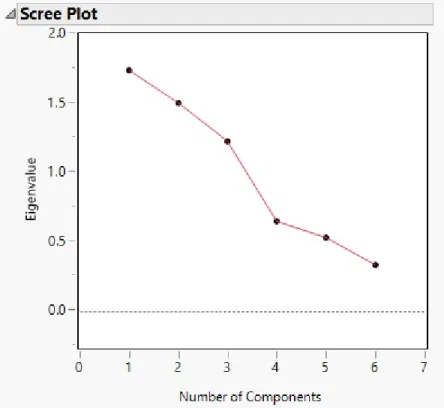
The principal components can be used as independent variables in a regression to model Overall Liking. The eigenvalues and scree plot, displayed in the figure below, can be used to determine the appropriate number of components to model in Principal Components Regression.

(34)

Figure 3.8: JMP: Scree Plot for PCA

An ideal scree plot would have a strong elbow- with early components decreasing quickly followed by latter components decreasing slowly. This strong elbow would show that the least important principal components all have low (and similar) eigen-values and are good candidates to remove from the analysis. However, the scree plot above does not fit the description of an ideal scree plot, as it is mostly linear and does not have a strong elbow. Thus it is difficult to determine from the scree plot the ideal number of components in the Bread PCA.

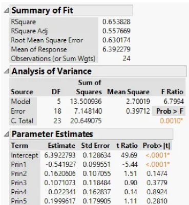
Side Note: After performing a PCA, the components can be used as the indepen-dent variables in a standard multiple linear regression model. This technique is called Principal Components Regression (PCR). To create a model that accounts for at least 90% of the variation in the X’s, Figure 3.5 indicates five variables must be included in the model. While it is ideal to reduce the model by more than one variable, it is

(35)

not possible in this example because the original Bread dataset independent variables were uncorrelated. The regression output modelingOverall Liking is displayed below in figure 3.9:

Figure 3.9: JMP: Principal Components Regression

The R2, RM SE, and parameter estimate for intercept are not much different the multiple linear and forward selection models from earlier. Also, the t-Ratio in the parameter estimates indicates that only the first principal component (Prin1) is significant in the model. Interpreting the regression model is much more difficult than assessing the goodness of fit because each independent variable is now comprised of a combination of the original variables. As mentioned in chapter 2, there are lengthy formulae for converting the components parameter estimates into estimates for the original variables. However, PCA is a better tool for independent variable analysis rather than regression. A dimension reduction substitute for PCR that also considers the dependent variable is the Partial Least Squares regression.

(36)

3.3.2 Partial Least Squares

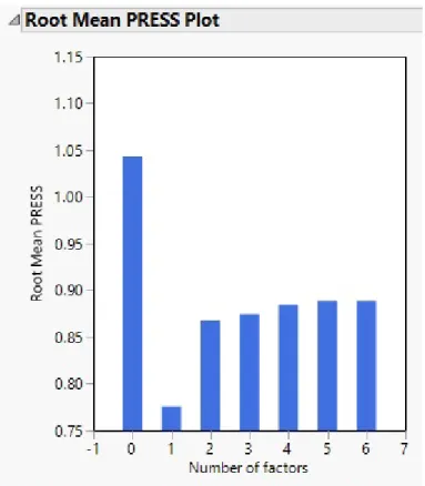
Like PCA,the Partial Least Squares (PLS) model is run using standardized vari-ables. The PLS model was created with the NIPALS specification using Leave-One-Out validation method1 (AIC is not an option for PLS) and maximum initial number of factors (which is equal to the number of independent variables, in this instance, 6). To determine the appropriate number of factors for the final model, the Root Mean PRESS Plot can be used:

Figure 3.10: JMP: Root Mean PRESS Plot

Root mean PRESS (predicted residual sum of squares) is a plot of the residuals corresponding to each number of factors (from 0 through the number of factors speci-fied prior to running the model). For this data, the best PLS model occurs when only

(37)

one factor is included, as it gives a root mean PRESS of 0.77577. PLS models with two or more factors have more than 0.85, as can be seen in the root mean PRESS plot.

Another option for selecting an appropriate number of factors is to use the ‘van der Voet T2_{’ in combination with root mean PRESS. The van der Voet} _Ts _number is a test statistic to determine if two models are differ significantly. [9] The number of factors with the lowest root mean PRESS has a van der Voet T2 p-value of 1.0. A model with fewer factors than the one with the lowest root mean PRESS can be selected if the van der Voet T2 _{indicates the model is not significantly different (a} common practice is to use a p-value greater than 0.1, as the van der Voet T2 _null hypothesis is not rejected). [9]

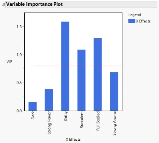
After selecting the number of NIPALS factors, there are a number of interesting and useful plots to use for analysis. One such plot is the Variable Importance Plot (VIP), shown in figure 3.11 below.

(38)

Figure 3.11: JMP: VIP Plot

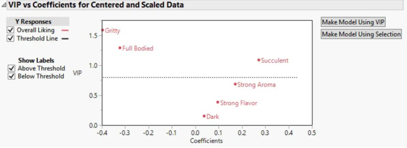
The VIP plot is a depiction of the VIP scores, which are a measure of each variable’s importance in measuring both X and Y. Typically 0.8 is used as the threshold for importance. Often, a small coefficient and a small VIP score is a good indication that a variable can be removed from the model. [9] This relationship can be seen in the ‘VIP vs Coefficients’ plot in figure 3.12. The VIP vs Coefficients plot includes the threshold line at 0.8, along with variables plotted as VIP (from figure 3.11) against coefficient value.

(39)

Figure 3.12: JMP: VIP vs Coefficients Plot

Variables below the threshold and near the center of the graph (in the above plot, the variables Dark, Strong Flavor, and Strong Aroma) are weak predictors of the de-pendent variable. The variables above the threshold can be used to develop multiple linear regression model, either directly or through additional forward selection.

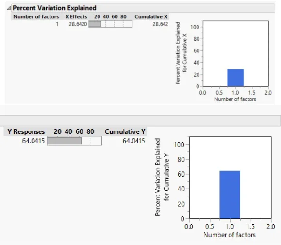
An additional useful statistic is the percent variation explained by the factors and theY variable response. In this PLS model, one factor explains 28.6% of the variation in X and 64% of the variation in Y, as shown in figure 3.13. In datasets larger than the Bread dataset, the percent variation can be used in the process to decide how many factors to model.

(40)

Figure 3.13: JMP: Percent Variation Explained Plots

After examining the various statistics produced by the PLS, a predictive model can be constructed using variable selection from the PLS output or by using the PLS centered and scaled model coefficients, displayed in figure 3.14.

(41)

Figure 3.14: JMP: Model Coefficients for Centered and Scaled Data

The centered and scaled output produces an intercept of 0 and comparatively large coefficients forGritty,Succulent, andF ullBodied. Both PCA and PLS provide procedures to produce information to reduce the dimension of a model but at the cost of a somewhat complex interpretation of the results.

3.4

Penalized Regression Models

3.4.1 LASSO

As with PCA, LASSO runs on standardized independent variables. Cross-validation is the most common technique for finding the bestλ value. However, for consistency and to compare results with previous models, this LASSO example was chosen using the AICc validation method. The following graph shows the AICc plotted against the magnitude of scaled parameters present in the model.

(42)

Figure 3.15: JMP: LASSO Solution Path

The lowest two AICc values occur when the parameters are scaled by a factor of three or by a factor of four. Because the objective is to simplify the model, select the option with three parameters. The estimates are displayed in figure 3.16 below:

Figure 3.16: JMP: LASSO Parameter Estimates

In the LASSO model,Gritty,Succulent, andF ullBodied were all included in the model, yet only Gritty is significant predictor. The β coefficients for Dark, Strong Flavor, andStrong Aroma have all been reduced toβi = 0. The intercept is similar to that of other models at approximately 6.4. The model summary in figure 3.16 below

(43)

details other summary statistics for the model. The AICc is close to AICc used in the forward selection model and the generalizedr2 _{is also comparable to the}_r2 _from other models. Overall, the LASSO model provides very similar results to previous models with the luxury of fewer variables.

Figure 3.17: JMP: LASSO Model Summary

3.4.2 Ridge Regression

While LASSO is able to perform selection by shrinking some of the X coefficients to 0, ridge regression is only able to perform shrinkage and not selection. The solution path highlights the ideal solution where the magnitude of the scaled parameters min-imizes the negative log likelihood (which is effectively maximizing likelihood). The solution path is displayed in figure 3.18 below:

(44)

Figure 3.18: JMP: Ridge Regression Solution Path

The parameters corresponding to this solution path are in 3.19. Because ridge regression does not select variables, all six are still present in the model. However comparing the coefficients to the multiple linear regression model, it can be observed that the coefficients for all the parameters, while consistent in direction, are all smaller in magnitude in the ridge model.

(45)

3.4.3 Elastic Net

The output for Elastic Net regression provides similar graphs and tables to that of the LASSO. The Solution Path in figure 3.20 below shows how the magnitude of scaled parameter estimates affects the AICc, which was the selected validation technique for this model.

Figure 3.20: JMP: Elastic Net Solution Path

The elastic net regression performs variable selection, and two variables shrink to 0. Looking at the parameter estimates of the remaining four variables, displayed in figure 3.21 below,Gritty is the only significant variable. The intercept is also similar to other models, with a value of approximately 6.4.

(46)

Figure 3.21: JMP: Elastic Net Parameter Estimates

The model summary in figure3.22 provides other statistics to compare the elastic net to other models. The AICc is similar to other models, as is ther2 value.

Figure 3.22: JMP: Elastic Net Model Summary

3.5

Summary of Illustrative Examples

The different selection and regularization techniques demonstrated in this chapter provide a brief example of how to interpret results. As can be seen from the param-eter and model summary outputs, the paramparam-eter estimates RMSE, and r2 values are similar. Thus for theBreaddataset, none of these techniques are statistically prefer-able and simplicity should take precedence. However, there are several advantages and disadvantages to each method, discussed in Chapter 4, that can provide some indication as to which method to use for a larger dataset.

(47)

Chapter 4:

Problems and Issues with

Each Approach

4.1

Multiple Linear Regression and Forward Selection

While multiple linear regression has a lengthy list of issues, the most significant in terms of this paper is that it does not translate well to large datasets. It is imprac-tical, and often mathematically impossible with regards to degrees of freedom, to use all independent variables and necessary interactions. A large number of independent variables also increases the risk of overfitting the model, where the model accurately reflects the patterns in the data but cannot accurately predict out-of-sample data. While there are many solutions to the issues with multiple linear regression, the most direct is to use a variable selection technique.

Forward selection models are also prone to overfitting the data. To minimize the risk of overfitting for both multiple linear regression and forward selection, models can be constructed using training and validation sets to assess the model’s predic-tive power. Another issue with forward selection is that the ‘mathematically best’ model could be due to chance.[7] Forward selection is an automated process that does not involve human judgment, so multicollinearity is another problem that can arise. However if correlations are examined prior to running the forward selection, it is simple to manually bypass any models that include highly correlatedXvariables.

4.2

PCA and PLS

There are two large problems with performing a Principal Components Analysis. The first is that PCA is an unsupervised learning technique. If the only objective is to strictly examine independent variables, unsupervised learning presents no issue.

(48)

However, if PCA will later be used as a predictive model, there is no guarantee that the components chosen to explain the variance in X will also explain the variance in Y. The second issue that arises with PCA is how to interpret the results of a regression with the components used as independent variables. The parameter coefficients output by a PCR do not directly translate back to the original variables. While formulae can be derived to interpret the coefficients, it is recommended to use PCA as a technique to examine correlations among the independent variables.

Because PLS is an iterative ordinary least squares sequence, it can be performed on matrices that have missing data. It can also be used on large datasets, especially performing well when there are more independent variables than records. However partial least squares cannot be used on binary, nominal, or ordinal data, nor can it predict non-linear relationships. [8] PLS has several different algorithms to choose from, so it requires more initial background knowledge than other predictive modeling techniques. However, one of the PLS algorithms (SIMPLS) is designed specifically to predict multiple dependent variables.

4.3

Penalized Regression Models

Penalized regression models, especially the LASSO and elastic net as they both perform variable selection, are suitable to use when the number of independent vari-ables exceeds the requirement. However, LASSO will only select at mostn variables, where n is equal to the number of records in the dataset. LASSO also fails to do grouped selection - if variables are grouped, the LASSO will often only select one variable from the group and ignore the others. Penalized regression models are eas-ier to interpret than PCA and PLS because they are the most similar to standard multiple linear regression. However penalized regression also lowers all β coefficients through the use of the penalty parameter, so interpretations must also account for this resulting bias. The tuning parameter can also create some issues for penalized

(49)

regression models. Selecting a tuning parameter that is too small will lead to overfit data, resulting in a model with high variance, and one that is too large will lead to underfit data. For a large dataset, ridge regression is unable to perform variable selection, as it does not shrink variables to 0.

(50)

Chapter 5:

Discussion

Any of the predictive modeling techniques described in this paper can be applied in the context of big data. However, depending on the raw data and the goal of the analysis, some methods may be more appropriate than others. The most important starting point is to examine the raw data carefully to assist in the decision-making process. Handling missing data and studying the pattern of missing data are essential precursory steps for any modeling. After looking at the data and undergoing initial data preparation steps (such as handling missing data, applying transformations, and standardizing variables), selective inference and dimension reduction techniques can be used independently or as supplements to each other as prediction tools. Table 5.1 briefly highlights each of the procedures.

Cross-validation has not been extensively discussed in the context of this paper. When working with big data, it is useful to partition the data into training and vali-dation sets in order to verify, and if necessary, to improve upon the chosen prediction technique. In the context of selective inference, cross-validation can ensure that a reduced model is providing an accurate prediction because there is true correlation between the variables rather than random chance.

After randomly partitioning data, the training set can be used to develop a model using one of the selective inference techniques discussed previously. Though big datasets often have many issues (missing data, correlation, size, etc.), considering dataset size and correlation can help narrow down selective inference techniques to try in the modeling process.

(51)

regression, forward selection, or ridge regression are simple in both computation and interpretation and could be reasonable options for predictive modeling. The defini-tion of ‘big data’ implies that there will generally be a large number of independent variables (maybe more independent variables than observations), so these are unlikely options for a final predictive model. A large number of independent variables indi-cates a model reduction process could be necessary; forward selection, PCA/PLS, or a penalized regression model (specifically LASSO and elastic net) are options to explore.

‘Are the independent variables correlated?’ As seen with the uncorrelated Bread

dataset in Chapter 3, PCA and PLS do not provide aid in dimension reduction if the variables are not highly correlated, as they are unable to group correlated variables into a single component. However, correlated independent variables can be examined using PCA. While it does not involve the relationship to the Y variable, PCA is a useful tool to initially explore correlations in more detail. PLS can be used for both study and predictive modeling, as it incorporates the dependent variable into the factor computation.

This thesis illustrated how various (currently popular) predictive modeling niques can be applied to ‘big datasets’ for variable selection. There are other tech-niques (neural networks, decision trees, and naive Bayes, to name a few) also gaining support. Some of these procedures provide automatic feature selection, have multiple tuning parameters, or may be more robust to variable selection. The field of ‘data analytics’ is expanding at a great rate, and as more technology is developed, the list of prediction techniques will continue to improve.

(52)

Summary of Advantages and Disadvantages for Each Selective Inference Technique Applied to Big Data Analysis

Multiple Linear Regression

Mathematically simple Impractical for big data

Easy to interpret coefficients Does not account for correlation Forward Selection

Simplified model Prone to overfitting

Principal Components Analysis

Correlated variables allowed Does not account forY variable

Large datasets possible Difficult to interpret components Partial Least Squares

Large datasets or missing data possible Complex interpretation

Multiple dependent variables possible No binary, nominal, or ordinal data LASSO Regression

Performs variable selection Selects at mostn variables

Easy to interpretβ coefficients Account for bias in interpretation Ridge Regression

Provides regularization Does not reduce the model Elastic Net Regression

Balances selection and regularization Account for penalties in interpretation Table 5.1: Summary of Selective Inference Techniques

(53)

Appendix A:

Original Data and Distributions

Overall Liking Dark Strong Flavor Gritty Succulent Full Bodied Strong Aroma

6.098 4.674 5.684 4.457 6.038 5.113 4.841 6.458 6.067 4.340 3.240 5.224 5.208 5.377 6.062 4.703 5.821 3.492 5.116 5.254 4.904 4.772 5.184 5.770 4.855 5.124 5.471 4.842 6.150 5.420 6.962 3.446 5.536 4.989 5.200 7.409 5.733 5.515 2.804 5.649 5.253 5.195 8.075 5.024 6.338 4.107 6.042 4.759 4.447 5.950 6.054 5.524 3.871 5.514 5.939 4.727 7.020 6.193 5.661 3.137 5.508 5.035 5.304 6.245 5.191 4.930 3.348 5.459 5.141 4.939 6.237 6.185 5.159 5.255 5.465 5.495 4.857 6.205 4.901 5.349 3.748 5.077 5.535 5.117 8.466 5.251 6.473 2.273 5.144 5.071 5.639 5.656 6.008 4.565 4.836 5.370 5.095 5.165 7.908 6.219 5.276 3.802 5.614 4.934 5.810 6.867 5.253 6.454 3.227 4.813 5.416 5.379 6.039 5.560 5.612 3.705 5.766 5.409 5.604 5.283 6.012 5.578 5.130 4.964 5.321 5.032 4.926 5.722 5.517 5.747 4.757 5.891 5.111 7.153 6.984 5.575 4.148 6.072 5.259 5.119 6.413 4.948 5.856 3.728 5.195 5.171 4.609 5.602 5.167 6.308 4.959 4.591 5.482 5.454 5.473 6.030 6.075 4.063 5.128 5.283 4.621 6.945 5.506 5.355 3.467 5.552 5.584 5.016

(54)

Original Data Distributions

Figure A.1: JMP: Distributions of Original Data

(55)

Appendix B:

Full JMP Outputs for All Models

Multiple Linear Regression

(56)

(57)

Forward Selection

(58)

(59)

Principal Components Analysis

(60)

(61)

Partial Least Squares

Figure B.7: JMP: Partial Least Squares Report

(62)

(63)

(64)

(65)

(66)

Figure B.18: JMP: LASSO Regression Report

Ridge Regression

(67)

Figure B.20: JMP: Ridge Regression Report

Elastic Net Regression

(68)

(69)

References

[1] Francis X. Diebold. A Personal Perspective on the Origin(s) and Development of ‘Big Data:’ the Phenomenon, the Term, and the Discipline. Technical report, University of Pennsylvania, 2012.

[2] Ian Guadard and Marie Cox. Discovering Partial Least Squares with JMP. SAS Institute, Cary, NC, 2013.

[3] Ron Klimberg and B. D. McCullough.Fundamentals of Predictive Analytics with JMP. SAS Institute, Cary, NC, 2016.

[4] Max Kuhn and Kjell Johnson. Applied Predictive Modeling. Springer Science + Business Media, New York, NY, 2013.

[5] Steve Lohr. The Origins of ‘Big Data’: An Etymological Detective Story. The New York Times, February 2013.

[6] James Manyika. Big Data: The next frontier for innovatoin, competition, and productivity. Technical report, McKinsey Global Institute, 2011.

[7] Minitab, Inc., State College, PA. Minitab 17, 2016.

[8] Giorgio Russolillo. Partial least squares algorithms for pca, component based regression and predictive path modeling. http://maths.cnam.fr/IMG/pdf/ Seminaire_Russolillo.pdf, Apr 2011.

[9] SAS Institute Inc., Cary, NC. JMP 12, 2015.

[10] Jonathan Taylor and Robert Tibshirani. Statistical Learning and Selective In-ference. Proceedings of the National Academy of Science, 112(25):7629–7634, 2015.

(70)

[11] Robert Tibshirani. Regression Shrinkage and Selection via the Lasso. Journal of the Roayl Statistical Society, 58(1):267–288, 1996.

[12] Pennsylvania State University. Applied data mining and statistical learning. Technical report, PSU, 2017.

[13] Hongquan Xu. Stat 105 chapter 12. Technical report, UCLA, 2012.

[14] Hui Zou. Regularization and variable selection via the elastic net. Technical report, Stanford University, 2005.

Electronic Theses and Dissertations

https://dsc.duq.edu/etd/182