TROY DAVIG, ERIC M. LEEPER, AND HESS CHUNG
Abstract. Interest rate rules for monetary policy and tax rules for fiscal policy change stochastically between two regimes. In the first regime monetary policy follows the Taylor principle and taxes rise strongly with increases in the real value of government debt; in the second regime the Taylor principle fails to hold and taxes follow an exogenous stochastic process.
Because agents’ decision rules embed the probability that policies will change qualitatively in the future, monetary and tax shocks always produce wealth effects, breaking down Ricardian Equivalence. The impacts of monetary policy shocks can also be different because their fiscal implications (and wealth effects) are different when regime can change. If monetary policy adjusts the interest rate at all in response to inflation, then i.i.d.policy shocks propagate for many periods.
The paper also addresses two empirical issues. First the “price puzzle” that plagues monetary VARs is a natural outcome of periods when monetary policy fails to obey the Taylor principle and taxes do not respond to the state of government in-debtedness. Second, dynamic correlations betweenfiscal surpluses and government liabilities, which have been interpreted as consistent with Ricardian Equivalence, can be produced by an underlying equilibrium that is non-Ricardian.
1. Introduction
Two themes run through policy analysis: rules determining policy choice are
func-tions of economic condifunc-tions; those rules may change over time. Those themes reflect
the common view that actual policy behavior is purposeful, rather than arbitrary, and that good policy adapts to changes in the structure of the economy or to
im-provements in understanding of how policy affects the economy.
Date: November 4, 2003. We thank Jon Faust, Dale Henderson, Lars Svensson and seminar participants at Banco de Portugal and the Federal Reserve Board for helpful comments. Affiliations: Davig, The College of William and Mary ([email protected]); Leeper, Indiana University and NBER ([email protected]); Chung, Indiana University ([email protected]).
c
°2003 by Troy Davig, Eric M. Leeper, and Hess Chung. This material may be reproduced for educational and research purposes so long as the document is not altered and this copyright notice is included in the copies.
A growing body of work estimates policy rules over different time periods to find
that critical parameters have changed in important ways over time.1 Those
parame-ters are critical because in simple theoretical models they can determine existence and uniqueness of equilibrium. In light of this evidence, there has been surprisingly little formal modeling of environments where regime change is stochastic and the objects subject to change are parameters determining how the economy feeds back to policy choice.
This paper allows interest rate rules for monetary policy and tax rules for fiscal
policy to change stochastically between two regimes. In the first regime monetary
policy follows the Taylor (1993) principle and taxes rise strongly with increases in the real value of government debt; in the second regime the Taylor principle fails to hold and taxes follow an exogenous stochastic process.
We are driven to model regime switching by our reading of American macro policies since World War II. Before describing the paper’s results, it is useful to review the history of monetary and tax policy behavior.
1.1. A Quick Post-WW II History of Regime Change. There is a near consen-sus among macroeconomists that U.S. monetary policy changed regime in late 1979. The consensus view holds that monetary policy changed from a period where
in-creases in inflation were passively accommodated to one where incipient inflation was
actively combatted with tighter policy.2 Taylor (1999a), Clarida, Gali, and Gertler
(2000), and Lubik and Schorfheide (2003b), among others, found that from 1960-1979 the Fed followed an interest rate rule that failed to satisfy the Taylor principle, which requires adjusting the Federal funds rate more than one-for-one in response to
inflation. Since the early 1980s, the Taylor principle is satisfied, according to this
empirical work.
Less well appreciated is the fact thatfiscal policy may also have experienced changes
in regime.3 In some periods, taxes are adjusted passively in response to changing
debt levels; at other times, tax changes are active attempts to achieve non-budgetary macroeconomic goals.
1For example, see Taylor (1999a) or Clarida, Gali, and Gertler (2000) for estimates of monetary
policy rules and Taylor (2000) or Auerbach (2002) for estimates of tax policy rules. Favero and Monacelli (2003) explicitly model regime switching in their estimates of monetary and tax policy rules.
2But see Bernanke and Mihov (1998), Sims and Zha (2002), and Hanson (2003) for alternative
viewpoints.
3This paragraph and the next draw on Pechman (1987), Poterba (1994), Stein (1996), Steuerle
The history of tax policy illustrates the pendulum swings in policy. In the 1950s taxes were increased three times on the grounds of budget balancing, in large part
tofinance the Korean War. By the 1960s, with the rise of Keynesian macro policies,
tax changes were initiated primarily as a countercyclical tool. Budget balance had slipped into the background of tax debates. This trend continued into the 1970s, with Presidents Ford and Carter proposing tax cuts designed to stimulate economic activity. Reagan’s Economic Recovery Plan drastically cut individual and corporate
income tax rates from levels that were thought to be adversely affecting incentives.
The resulting explosion in Federal government debt and its associated interest pay-ments shifted priorities once again toward budget balancing, and in 1982, 1984, 1990, and 1993 Reagan, Bush, and Clinton signed legislation that raised taxes to reduce
budget deficits. During the 2000 presidential campaign, George W. Bush ran on a
plank that taxes should be cut “to return the budget surplus to the people.” By the
time Bush’s campaign pledge was ratified by Congress in 2001, the rationale for tax
reduction had shifted once again–this time from budget concerns to economic stimu-lus. The last two tax reductions, the Job Creation and Worker Assistance Act (2002) and the Growth and Jobs Act (2003), were unambiguously motivated by
countercycli-cal objectives. Evidently over the past 50 years fiscal policy behavior has fluctuated
between periods when taxes were adjusted in response to the state of government indebtedness and those when other priorities drove tax decisions.
1.2. What We Do. Against this history of shifts in policy rules, we use a very
simple model as afirst step toward examining the implications of the kinds of regime
changes that the United States has actually experienced. The stark model highlights mechanisms that arise from regime switching but will continue to be present in richer models where the mechanisms are harder to isolate.
Because agents’ decision rules embed the probability that policies will change
qual-itatively in the future, monetary and tax shocks always produce wealth effects.
Re-gardless of the prevailing regime, agents never expect the changes in debt that policy
disturbances induce to generate offsetting changes in future taxes. Those wealth
ef-fects mean that taxes always matter for aggregate demand and Ricardian Equivalence
breaks down. The impacts of monetary policy shocks can also be different because
their fiscal implications (and wealth effects) are different when regime can change.4
We also show that if monetary policy adjusts the interest rate at all in response to
inflation, then i.i.d. policy shocks propagate for many periods, creating serial
corre-lation in inflation and nominal interest rates.
4Thefiscal consequences of monetary policy are stressed in the optimal policy work of Benigno
The paper uses simulated time series from the model to address two empirical issues. First, the “price puzzle” that plagues monetary VARs is a natural outcome of periods when monetary policy fails to obey the Taylor principle and taxes do not respond to the state of government indebtedness. Second, dynamic correlations
between fiscal surpluses and government liabilities, which have been interpreted as
consistent with Ricardian Equivalence, can be produced by an underlying equilibrium that is non-Ricardian.
This pattern of results raises two questions. Is Ricardian equivalence a useful benchmark for the study of tax policy? Can we rely on the Taylor principle to insult
the economy from the inflationary consequences of fiscal policy?
2. Contacts with the Literature
This paper makes contact with existing work in several areas. Sargent and Wallace
(1981) were among thefirst to emphasize intertemporal aspects of monetary andfiscal
policy interactions. With monetary andfiscal policy, there are two policy authorities
that jointly determine the price level and ensure the government is solvent. When one policy authority pursues its objective unconstrained by the behavior of the other authority, its behavior is “active,” whereas the constrained authority’s behavior is
“passive.”5
If policy regime isfixed, active monetary policy coupled with passivefiscal policy–
the policy mix implicit in the literature on the Taylor principle–produces monetarist
and Ricardian predictions of monetary and fiscal policy impacts. In contrast, when
active fiscal policy combines with passive monetary policy–the combination
associ-ated with the fiscal theory of the price level6–monetary and tax changes generate
wealth effects that shift aggregate demand, and policy impacts are non-monetarist
and non-Ricardian.
Lucas (1976) taught macroeconomists to think about policy changes in terms of shifts in regime. But Lucas’s examples all involve once-and-for-all changes, rather than the on-going process described in the quick history above. Cooley, LeRoy, and Raymon (1982, 1984), among others, have argued that treating policy as making once-and-for-all choices is logically inconsistent. After all, if policy authorities can contemplate changing regime, then regime is not permanent. If there has been a
history of changes in monetary and fiscal policy regimes, private agents will ascribe
a probability distribution over policy regimes. Agents’ expectations, and therefore
their decision rules, will reflect their belief that policy changes are not
once-and-for-all. This point resonates especially crisply in the United States, where the policy 5This follows Leeper’s (1991) taxonomy.
changes we aim to model are intrinsically temporary; they arose largely because of the personalities of the political players, rather than through the creation of new policy institutions or changes in existing institutions’ legal mandates.
A growing number of empirical studies finds evidence of regime changes. Clarida,
Gali, and Gertler (2000) find that from 1960-1979 the Taylor principle does not hold
for U.S. monetary policy. They implicitly assume thatfiscal policy was passive during
this period, allowing for multiple equilibria, and they interpret the inflation of the
1970s as arising from self-fulfilling sunspot equilibria. Woodford (1999) suggests that
fiscal policy may have been active during that period, implying that observed inflation
emerged from a unique equilibrium. Favero and Monacelli (2003) and Sala (2003) offer
empirical evidence that fiscal policy was active and monetary policy was passive in
the 1960s and 1970s, supporting Woodford’s argument.
All this work is couched in terms of changes in policy regime, and there have been
some efforts to incorporate switching policy specifications into dynamic stochastic
general equilibrium (DSGE) models to study the fiscal theory of price level
determi-nation (FTPL) [for example, Sims (1997), Woodford (1998), Loyo (1999), Mackowiak (2002), Weil (2003), and Daniel (2003)]. But each of these papers considers only one-time changes in regime. In addition, Loyo (1999), Weil (2003), and Daniel (2003)
consider only changes infiscal regime, holding monetary policy behaviorfixed. Given
a history of both monetary andfiscal regime switching, it is important to allow both
policies to change. This paper generalizes the theoretical literature on monetary and
fiscal policy interactions by explicitly modeling regime change as an on-going process.
Both one-time changes in regime and changes in only fiscal or monetary policy
be-havior are special cases of our specification.
There is work that models on-going regime change [for example, Andolfatto and Gomme (2003), Davig (2002, 2003b), Leeper and Zha (2002), Schorfheide (2003), and Andolfatto, Hendry, and Moran (2002)]. That work considers only exogenous processes for policy variables that switch regime. This paper makes substantive and technical contributions by extending work on on-going regime change to allow the objects subject to change to be parameters that determine how the economy feeds
back to policy choice. This is thefirst example of which we are aware that allows for
regime switching in parameters of endogenous policy rules in a DSGE model, where the parameters determine existence and uniqueness.
Empirical findings that policy regimes have changed in important ways are diffi
-cult to interpret without theory that models regime changes explicitly [Favero and
Monacelli (2003) and Sala (2003)]. This paper fills some of the theoretical holes.
Finally, the paper connects to two bodies of empirical work. It offers an
forth by Barth and Ramey (2001) and Christiano, Eichenbaum, and Evans (2001). The paper also provides a counterexample to the empirical inferences drawn by Bohn
(1998) and Canzoneri, Cumby, and Diba (2001) about the behavior offiscal policy in
the United States.
3. The Model
The model is an endowment version of Sidrauski (1967), modified to include an
interest rate rule for monetary policy and a tax rule for fiscal policy.
3.1. Households. The representative consumer receives a constant endowment each
period, yt =y, of which a constant gt = g is consumed by the government. Agents
choose consumption,ct,and decide how to allocate portfolio holdings between values
of money, mt=Mt/Pt, and bonds, bt =Bt/Pt. The household’s problem is:
maxE0 ∞ X t=0 βt[log(ct) +δlog (mt)], (1) subject to ct+mt+bt+τt =y+ mt−1 πt +Rt−1 bt−1 πt , (2)
where0< β <1is the discount rate,δ >0, Rt−1 is the one-period return on nominal
bonds, τt is lump-sum taxes, and πt =Pt/Pt−1. The household takes initial nominal
assets as given: M−1 >0, R−1B−1 >0.Expectations at datet are taken with respect
to an information set that contains all variables datedt and earlier. Policy is the sole
source of uncertainty, as detailed below.
In equilibrium,ct=c=y−gand thefirst-order necessary conditions corresponding
to the Fisher and money-demand relations reduce to
1 Rt =βEt · 1 πt+1 ¸ , (3) mt=δc · Rt Rt−1 ¸ . (4)
The optimal paths for real balances and bonds must also satisfy their respective transversality conditions.
3.2. Policy Specification. The fixed-regime model corresponds to Leeper (1991), where the properties of the rational expectations equilibrium depend on the reaction
coefficients in the monetary andfiscal policy rules. The fixed-regime rules are
τt =γ0+γbt−1+ψt, (6)
where θt andψt arei.i.d. shocks to monetary and tax policies.
We choose these policy rules to connect this paper to existing work. In this economy with perpetually full employment, an interest rate rule for monetary policy is clearly
not optimal. If anything, it will reduce private welfare. We employ specification (5)
for two reasons. First, it closely resembles monetary policy rules that have received detailed study in recent years [for example, Taylor (1999b)]. Second, (5) produces features of an equilibrium that will continue to hold in models with frictions where rules from the general class to which (5) belongs are optimal. The form of the tax rule, (6), is also widely used in both model simulations [Bryant, Hooper, and Mann
(1993)] and in analytical studies of monetary and fiscal policy interactions [Leeper
(1991), Sims (1997), or Woodford (2003)].
A combination of lump-sum taxes, new one-period nominal bonds and money
cre-ationfinance government purchases and debt payments. The government’sflow
bud-get identity holds at each date t≥0:
Bt+Mt Pt +τt=g+ Mt−1 +Rt−1Bt−1 Pt , (7)
given initial nominal liabilitiesM−1 >0, R−1B−1 >0.7
In a linear approximation to the model, a monetary authority reacting aggressively
to inflation, |αβ|>1, and afiscal authority raising taxes sufficiently to cover interest
payments and principle on the debt, ¯¯β−1−γ¯¯ < 1, implies a unique equilibrium
consistent with Ricardian equivalence.8 This policy combination is referred to as
active monetary and passive fiscal policy (AM/PF). A monetary authority reacting
weakly to inflation, |αβ| < 1, and a fiscal authority reacting weakly to real debt,
¯¯β−1−γ¯¯ > 1, implies a unique equilibrium where the path of taxes affects the
inflation rate. This policy combination is referred to as passive monetary and active
fiscal policy (PM/AF). One version of the fiscal theory of the price level emerges as
the special case α=γ = 0.
7By assuming initial government debt is positive, we do not address the criticism that the FTPL
falls apart whenB−1= 0.The criticism is made in a perfect foresight model by Niepelt (2001) and
countered in a stochastic model with incomplete markets by Daniel (2003).
8Logarithmic preferences make money essential and eliminate Obstfeld and Rogoff’s (1983)
spec-ulative hyperinflations as potential equilibria. This allows the Taylor principle, coupled with passive tax policy, to deliver uniqueness. As Sims (1997) shows, if money is inessential, this policy mix does not produce a determinant equilibrium.
The policy specification for the regime-switching model allows the coefficients in the tax and interest rate rules to depend on an observed state variable. The regime-switching policy rules are
Rt = α0(St) +α1(St)πt+θt, (8)
τt = γ0(St) +γ1(St)bt−1+ψt, (9)
where St∈{1,2}, θt∼N(0, σ2θ) and ψt ∼N(0, σ2ψ). The reaction coefficients take a
different value depending on the state variable,
γi(St) = ½ γi(1) forSt = 1 γi(2) forSt = 2 , for i={0,1}, (10) αj(St) = ½ αj(1)for St= 1 αj(2)for St= 2 , for j ={0,1}. (11)
We use the local results from the linearized (fixed-regime) model to guide
para-meter choices for the non-linear switching model. For most of this paper regime 1
combines active monetary policy with passive fiscal policy (AM/PF): |α1(1)β| > 1
and ¯¯β−1−γ1(1) ¯
¯<1.Regime 2 combines passive monetary policy with active fiscal
policy (PM/AF): |α1(2)β|<1 and¯¯β−1−γ1(2)¯¯>1.
Regimes follow a two-state Markov chain governed by the transition matrix
Π= · p11 1−p11 1−p22 p22 ¸ , (12) P [St=j|St−1 =i] =pij, where i, j = 1,2 and p12≡1−p11 andp21 ≡1−p22.
We assume agents observe current and past realizations of regimes and of exogenous disturbances.
Although our reading of macro policy history and Favero and Monacelli’s (2003)
estimates suggest that monetary andfiscal policy have not switched synchronously, for
two reasons we assume that they do through most of the paper. First, it is a reasonable
first step toward understanding the implications of regime switching. Second, full
non-synchronous switching would allow the economy to evolve for a time under policies that are both passive. A PM/PF mix, if it were expected to last forever, yields indeterminacy of equilibrium. We postpone grappling with the numerical aspects of indeterminacies and sunspots in non-linear models to later work. Section 6, however, displays an example of non-synchronous switching in a case where the equilibrium is unique.
3.3. Competitive Equilibrium. The equilibrium for the economy with
regime-switching policy rules is defined as:
Definition 1. Given the state vector Φt = {wt−1, bt−1, θt, ψt, St}, where wt−1 =
Rt−1bt−1 +mt−1, a competitive equilibrium for the economy consists of a con-tinuous decision rule for real debt, bt = hb(Φt), and a continuous pricing function,
πt =hπ(Φt), such that
(1) taking sequences {Rt, τt, πt, θt, ψt, St} as given, the representative agent’s op-timization problem is solved;
(2) thefiscal authority setsτt according to (8)and the monetary authority setsRt according to (9);
(3) the government budget identity, (7), and the aggregate resource constraint,
yt =ct+gt, are satisfied.
With a fixed endowment of goods each period, it is not feasible for the real value
of government debt to grow without bound even though in a growing economy debt can expand at a rate less than the real interest rate without violating the agents’ transversality condition for debt. Hence, in a deterministic steady state, all real
values of variables, the nominal interest rate, and the inflation rate are constant.
4. A Benchmark Specification
It may seem natural to solve the model by first linearizing around the
regime-dependent steady states. But in the switching model, policy parameters as well as policy shocks are random variables. For some policies of interest it can turn out that
the one-step-ahead forecast error in inflation from the Fisher relation is correlated with
future policy parameters. Linear methods fail to capture this correlation, leading the approximations to incorrectly classify existence and uniqueness of equilibrium.
Appendices A-C show this in detail for two different linearization methods. Appendix
D describes the numerical procedure for solving the non-linear switching model. In
all the results reported, we confirm local uniqueness of decision rules by randomly
perturbing the converged rules and checking that the algorithm recovers those original decisions.
This section describes results from a benchmark specification that is designed to
build intuition about the nature of the switching equilibrium. The section also
con-trasts the results with predictions from the model with fixed policy regime.
4.1. Parameter Selections. Our objective is to obtain qualitative, rather than quantitative, implications from the model, and the parameter values were chosen with that aim in mind. Several parameter choices were based on their implications
for the model’s deterministic steady state, which we set equal across regimes.9 We
take the model to be at an annual frequency, so we set β = .9615, implying a 4
percent real interest rate. Output is normalized to 1 and government consumption
is 25 percent of GDP. The debt-output ratio is .4 and inflation is 3 percent in the
deterministic steady state; both numbers are in the ballpark for post-war U.S. data.
In choosing the weight on real money balances in preferences, δ, we sought to make
the model’s consumption velocity close to U.S. data.10 This implied δ=.0296.
The feedback parameters in the policy rules, (α1(St), γ1(St)), were chosen to
cor-respond to values used in the literature. In regime 1–active monetary policy and
passive fiscal policy–α1(1) = 1.5, a common value in the Taylor rule literature, and
γ1(1) =.275, implying a very strong response of taxes to debt. In regime 2–passive
monetary policy and active fiscal policy–we chose the rules most often analyzed in
the FTPL literature: α1(2) = 0andγ1(2) = 0,making both the nominal interest rate
and taxes exogenous.
Given the settings for (α1(St), γ1(St)) and the assumptions on the deterministic
steady state values for debt and inflation, the intercept terms for the policy rules,
(α0(St), γ0(St)),are determined.
For the benchmark specification, we make the transition probabilities between
regimes equal, with the regimes only moderately persistent. Withp11=p22=.85,the
average regime duration is 6-2/3 years. This duration is briefer than seems plausible,
but it makes the differences between regimes clear.11
The variances of the i.i.d. policy shocks, (θt, ψt), are fixed across regimes. We set
σ2
θ = 3.125e−6andσ2ψ = 2.05e−5.
12 A constantσ2
ψ implies the same-sized tax shock
in each regime: two standard deviations amount to a change in taxes relative to its
stationary mean of about 3-1/2 percent. Because of simultaneity between Rt and πt
in the monetary policy rule, a constant σ2
θ can imply very different changes in the
nominal interest rate and inflation from a given shock. In the benchmark model, a
two standard-deviation shock to θt lowers Rt 5 basis points in regime 1 and 35 basis
points in regime 2.
9Of course, in the stochastic regime-switching model, the higher moments that matter for expected
inflation can vary across regime. Consequently, the means of the stationary distribution conditional on either regime will not match their deterministic steady state counterparts.
10The average ratio of consumption of non-durables plus services to the real monetary base over
1959-2002 is about 2.4.
11In section 5 we examine the equilibrium’s sensitivity to variation in policy settings, including
feedback parameters and regime duration.
12For present purposesfixing variances across regime is unobjectionable, but for matching data it
may be a problem, as the work by Bernanke and Mihov (1998), Sims (1999), Sims and Zha (2002), Hanson (2003), and Favero and Monacelli (2003) suggests.
4.2. Non-linear Impulse Response Analysis. The methods of Gallant, Rossi,
and Tauchen (1993) are used to assess the dynamic impacts of shocks to fiscal and
monetary policy. Impulse response functions reported below contrast the conditional
mean profile of a series to a baseline profile. A regime-dependent steady state is
defined as follows.
Definition 2. A regime-dependent steady state, ©π(j), b(j)ª, is values for the state vector such that
¯ ¯[πt, bt]0 ¯ ¯−¯¯[πt−1, bt−1]0 ¯ ¯< and St−1 =St=j,where j ={1,2}.
For example, the impact effect of an i.i.d shock to lump-sum taxes on inflation
conditioning on an AM/PF policy (regime 1) is described by
b πt=hπ ¡ w, b,0, ψt,1 ¢ −hπ¡Φ¢, (13)
where hπ¡Φ¯¢ is the regime-dependent steady state value for inflation. The paths for
inflation and debt are then recursively updated, holding regime constant. The
non-linear impulse response is the conditional path less the baseline path. The impulse response analysis that follows uses derivations analogous to (13) to trace out the
impacts of perturbing on shock, holding all other sources of randomnessfixed.
4.3. Average versus Marginal Sources of Financing. This paper follows Sargent
and Wallace (1981) by emphasizing the fiscal financing consequences of alternative
monetary and tax policy rules. We wish to highlight a distinction that does not
appear in Sargent and Wallace: there can be an important difference between the
average and the marginal source of financing.13 In the model’s deterministic steady
state direct taxation through τ constitutes over 96 percent of total revenues, leaving
seigniorage to cover a little over 3 percent. Although the means of the stochastic
steady states across regimes differ slightly from the deterministic steady state values,
the message is the same: on average seigniorage is a trivial source offiscalfinancing.
In regime 1 (AM/PF), seigniorage averages about 3.6 percent of total revenues (.99 percent of output), and in regime 2 it averages 3.4 percent (.95 percent of output). These numbers are consistent with the evidence King (1995) cites.
13This distinction is sometimes overlooked. King and Plosser (1985), for example, point to the
fact that averaged across time inflationfinancing is a trivial source of revenues in the United States as suggesting that inflation taxes should also be inconsequential in response to various shocks to the economy. In addition, many observers dispute the relevance of the dynamic policy interactions that Sargent and Wallace describe on the grounds that over time most developed countries do not rely heavily on seigniorage revenues [King (1995)]. Castro, Resende, and Ruge-Murcia (2003) draw a similar conclusion for OECD countries.
There are three distinct marginal sources offinancing that exogenous disturbances
may generate. The first arises from an instantaneous jump in the price level that
revalues existing nominal government liabilities. The other two sources are dynamic, arising from changes in the present values of the primary surplus and seigniorage.
Define the present value of the primary surplus as
xt= ∞ X s=0 "Ã s Y j=0 πt+j+1R−t+1j ! (τt+s+1−g) # (14) and the present value of seigniorage as
zt = ∞ X s=0 "Ã s Y j=0 πt+j+1R−t+1j ! ¡ mt+s+1−mt+sπ−t+1s ¢# . (15)
The government’s present value budget identity implies
Bt
Pt
=xt+zt. (16)
After taking expectations at datet of both sides of 16, Cochrane (2001b) refers to
this relationship as a “debt valuation equation,” which he uses to exposit the FTPL.
When expectedxt and zt are fixed by policy behavior, a bond-financed tax cut must
make Pt jump to ensure the equilibrium value of debt does not change. This is the
instantaneous marginal source of financing.
Under different policy assumptions, exogenous shocks may bring forth expected
changes in xt or zt. Given the benchmark parameters, when regimes are permanent,
i.i.d.shocks to taxes and to monetary policy generate no change in the present value of
seigniorage in regime 1 (AM/PF), though they do affect the present value of surpluses.
Tax shocks in regime 2 (PM/AF) leave both xt and zt unchanged, while monetary
policy shocks change both xt and zt. In contrast, in the switching model only tax
disturbances in regime 2 leave the present values in (14) and (15) unchanged.14
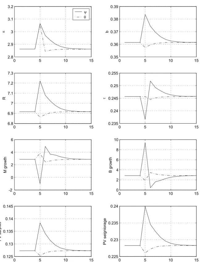
4.4. Impacts of Policy Shocks in Regime 1 (AM/FP). To isolate the impacts
of fiscal and monetary policy shocks, we condition on regime, start the economy at
its steady state for that regime, perturb either ψt or θt, and compute the change
in the decision rules and the resulting changes in path of variables, as indicated in
(13). Regime is held fixed in this experiment. The impacts are reported infigures 1
(conditioning on regime 1) and 5 (conditioning on regime 2); solid lines are responses
to an i.i.d.tax cut and dashed lines are responses to an i.i.d. monetary easing.
14If regime 2 setγ
4.4.1. Tax Shocks. Regime 1 fiscal policy would be Ricardian if policy regime were
expected to last forever. A bond-financed tax cut brings forth an expectation of future
taxes whose present value exactly equals the increase in the value of debt. With no change in net wealth, demand for goods is unchanged at initial prices and interest
rates. Unchanged inflation implies unchanged nominal rates, leaving the present value
of seigniorage also unchanged.
When regime can change, agents treat a tax cut as an increase in wealth because they place positive probability on switching to regime 2 (PM/AF), where taxes are
exogenous. A switch to regime 2 withfixed taxes brings with it a discrete devaluation
of government debt through an increase in the price level. Higher wealth increases
aggregate demand and the current inflation rate in this economy with afixed supply
of goods [figure 1].15
Withα1(1) = 1.5in regime 1, monetary policy reacts to the higher inflation rate by
sharply raising the nominal interest rate. This creates an expectation that inflation
will remain above its stationary level in regime 1, which is consistent with the antic-ipated debt devaluation. With the impulse response functions conditional on regime 1, active monetary policy propagates the transitory tax cut, generating persistently
higher inflation and nominal rates. The persistence is so strong that variables remain
away from their pre-shock levels over 10 periods after the tax cut.
In periods following the tax cut, taxes increase in a manner suggestive of Ricardian
fiscal behavior, as regime 1 policy passively raises taxes when debt increases. But
the rise in the value of debt exceeds the present value of these tax increases, with the
difference made up by an increase in the present value of inflation taxes.
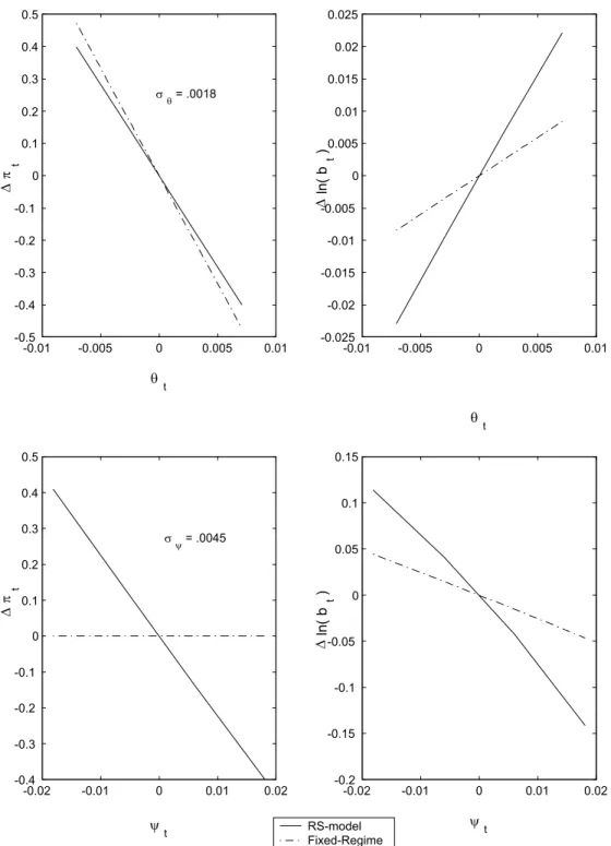
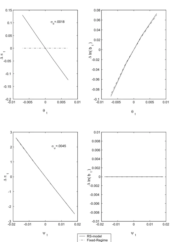
Decision rules in the switching environment differ markedly from the rules when
regime is fixed. Figure 2 shows the equilibrium rules for bt and πt under AM/PF
policies for both fixed and switching regime models. The rules are expressed as
functions of ψt and θt, holding all other state variables at their regime-dependent
steady state values. The lower left panel of thefigure illustrates the contemporaneous
impacts of taxes on inflation. When regime is permanent Ricardian equivalence makes
taxes irrelevant, but taxes matter when regimes can change.
15Some readers might object that this result seems to be inconsistent with Canzoneri, Cumby,
and Diba’s (2001) proposition stating that if surpluses respond positively to debt infinitely often– however briefly and weakly–then the equilibrium is Ricardian. But the relevance of the sufficient conditions in the proposition can be questioned. The proposition presupposes that debt can grow without bound and not lead to non-Ricardian policy. But this necessarily implies that taxes, which are proportional to debt, also must grow without bound. In our model, or any model with distorting taxes, this cannot happen so the proposition does not apply [also see Cochrane (2001b)]. We thank Chris Sims for bringing this to our attention.
Regime switching also increases the elasticity of real debt to policy disturbances by propagating the shocks’ impacts and changing the present values of taxes and
seigniorage [right panels of figure 2]. For example, as figure 1 showed, a negative
shock to ψt raises the nominal interest rate and generates an expectation that both
direct and inflation taxes will rise in the future, supporting the increase in the current
value of debt. Of course, the higher value of debt is associated with a higher present value of surpluses when the switching model conditions on staying in regime 1 where
γ1(1) = .275. Figure 3 shows the present values of both surpluses and seigniorage in
the switching and the fixed-regime models.
If agents expect tax policy to be non-Ricardian in the future, the Taylor principle
may not be sufficient to offset the inflationary impacts of tax disturbances. Indeed,
the Taylor principle is destabilizing because it givesi.i.d.tax shocks persistent effects,
increasing the variances of demand and inflation.
4.4.2. Monetary Shocks. When regime 1 is fixed, a transitory monetary policy shock
creates a one-time increase in inflation by the conventional mechanism of an increase
in liquidity. The Taylor principle ensures the nominal interest rate stays fixed. A
decline in the value of debt is matched by a decline in the present value of surpluses,
guaranteeing that both wealth and future inflation taxes are constant.
Regime switching alters the effects of a transitory monetary easing by expanding
liquidity and reducing wealth [figure 1]. Because agents anticipate policy will shift to
PM/AF, they no longer expect lower future taxes to match the decline in debt’s value; wealth falls. Lower wealth attenuates the liquidity-induced expansion of demand.
Along with the expectation that fiscal policy will switch to exogenous taxes comes
the expectation of a discrete drop in the price level to revalue debt. The present value
of seigniorage and the current nominal interest rate fall accordingly. Lower financial
wealth at the beginning of next period, with no new injections of liquidity, reduces
inflation in that and subsequent periods.
Note that the monetary shock generates a small “price puzzle”: a monetary easing
that lowers the nominal interest rate is followed by lower future inflation. As we
see below, this pattern emerges because agents perceive there is a chance policy will change to regime 2 in the future.
When prevailing policies combine AM and PF, tax disturbances produce a negative
correlation between money growth and inflation, and a positive correlation between
nominal debt creation and inflation. Monetary policy shocks make money growth
and inflation positively correlated, but bond growth and inflation are negatively
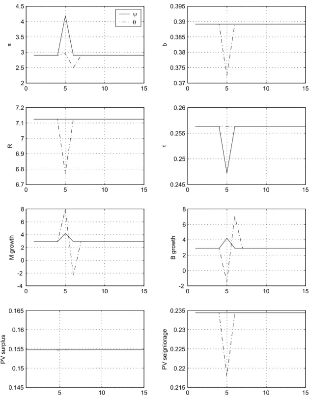
4.5. Impacts of Policy Shocks in Regime 2 (PM/AF). Regime 2 policy behav-ior corresponds to the standard FTPL exercise: both taxes and the nominal interest rate are exogenous. The policies also satisfy the hypotheses of Sargent and Wallace (1981) with the obvious, but crucial, exception that government debt is nominal in this model, but indexed in Sargent and Wallace’s.
4.5.1. Tax Shocks. A permanent regime 2 is the canonical FTPL exercise. Fixed
future taxes and constant current and future interest rates mean that a tax cut
cannot be financed by future revenues. At initial interest rates and prices, agents
feel wealthier and try to increase their consumption paths. This increase in demand drives up the current price level until the value of debt is returned to its original level
and agents are happy with their initial consumption plans. By fixing the interest
rate, monetary policy prevents the tax shock from propagating.
Regime switching does not alter the fixed-regime results [figure 5]. The current
inflation rate jumps to devalue the newly issued nominal debt; on the margin, the
full tax cut is financed by contemporaneous surprise inflation taxes. An unchanged
value of debt is consistent with unchanged present values of taxes and seigniorage. Money growth reacts passively to the higher price level to ensure the money market
clears at the fixed nominal interest rate. These effects coincide with those under
a fixed PM/AF regime because even though agents impute a positive probability
to a Ricardian tax rule and a Taylor rule in the future, unchanged real debt and an unchanged present value of surpluses are consistent with such a switch in rules.
Indeed, the decision rules as a function ofψt are identical [figure 6].
4.5.2. Monetary Shocks. When regime 2 is fixed, a monetary policy shock at time
t lowers the nominal interest rate and induces offsetting portfolio substitutions by
agents out of debt and into money. With their budget sets unperturbed by the shock,
there is no change in aggregate demand or inflation initially. The lower nominal rate
creates an expectation of lower future inflation and, therefore, seigniorage revenues
(supporting the drop in the value of debt). How is the lower expected inflation
realized? Although changes in real balances and real debt offset each other, the drop
inRt makes financial wealth,wt, lower at the beginning of periodt+ 1. This reduces
demand and inflation in that period.
When regime can switch, surprise monetary easing produces a similar pattern of
impacts. The only difference is the small contemporaneous uptick in inflation [figure
5], which arises because agents impute a positive probability to switching to regime
1 (AM/PF), where expansionary monetary policy raises inflation.
With monetary policy in this model couched in terms of an interest rate rule, the expansionary monetary shock produces a sizeable “price puzzle.” As we explore
in section 7, this pattern of correlation offers an explanation for the “price puzzle”
findings in the monetary VAR literature.
In regime 2, tax shocks make inflation positively correlated with both money growth
and bond growth. As in regime 1, monetary policy disturbances create a positive
correlation between money and inflation and a negative correlation between debt and
inflation.
5. Exploring the Parameter Space
This section characterizes the implications of alternative parameter settings across two important dimensions of the parameter space. First we show in regime 1 (AM/PF)
the implications of the expected duration of each regime as reflected by the transition
matrix. The benchmark settings for the PM/AF regime assume the monetary
author-ity sets interest rates independently of inflation, implying tax reductions are financed
entirely by a contemporaneous inflation tax (as in the FTPL). The implications for
the dynamic responses to tax shocks when interest rate policy responds positively,
but passively, to inflation are the second dimension we explore.
5.1. An Active Monetary/Passive Fiscal Regime. As section 4 demonstrated, agents’ expectations that regime will switch in the future play a crucial role in
deter-mining the impacts of policy disturbances. The benchmark specification assumes that
both regimes are relatively persistent. Here we explore how regime duration affects
the result that tax cuts generate wealth effects in regime 1. The expected duration
of a regime is given by
E[dj|St=j] = 1 1−pjj
,
for j = {1,2} and dj = T −t, where St = St+1 = · · · = St+T = j and St+T+1 6= j.
By relatively persistent we mean thatp11 > .5andp22 > .5. These restrictions create
the expectation that regimes will be in place for more than two periods, making it reasonable to interpret impulse responses that condition on staying in a particular regime for several periods.
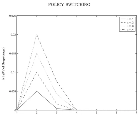
The degree to which tax shocks affect inflation in an AM/PF regime depends on
the transition matrix. Figure 7 illustrates how the magnitude of the impact of a
tax cut on inflation increases as p11 →0 andp22 → 1. Each decision rule represents
different probabilities in the transition matrix, where
λ= E[d1|St= 1]
E[d1|St= 1] +E[d2|St= 2]
represents the proportion of time spent in the AM/PF regime. As the expected
disturbances increase because agents expect to switch to the PM/AF regime in the future and then remain there relatively longer than in the AM/PF regime.
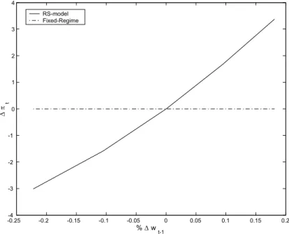
As figure 8 illustrates, the transition matrix affects the elasticity of inflation with
respect to a tax cut. The paths for inflation condition on the AM/PF regime and use
that regime’s steady state as the baseline; the tax cut occurs in period 2. As agents expect to spend relatively more time in the PM/AF regime, a tax cut generates
a larger increase in inflation on impact and results in higher variance of inflation.
The larger increase on impact arises from the expectation of a regime change to a more persistent PM/AF regime in the near future. Consequently, agents expect to remain in the AM/PF regime for relatively fewer periods, creating a lower expected present value of direct taxes relative to a scenario where the AM/PF regime is highly persistent. Thus, the expected regime change, which would result in a discrete jump
in the price level, generates expectations of higher inflation relative to where agents
expect to remain in the AM/PF regime for several periods.
5.2. A Passive Monetary/Active Fiscal Regime. In the fixed-regime model, a tax shock moves the price level and revalues outstanding nominal debt so the value of real debt matches the discounted value of future surpluses and seigniorage. With exogenous taxes and a pegged interest rate, the revaluation of nominal debt following an i.i.d. shock to taxes occurs instantaneously. But when regime is fixed, transitory
tax shocks can generate serially correlated changes in inflation if the monetary
au-thority responds weakly to inflation (α1 >0). This prevents the complete devaluation
of nominal debt from occurring in the period of the tax shock. Instead, a tax cut is
financed by issuing debt that will be repaid with inflation taxes spread over several
future periods.
Asαincreases, the monetary authority responds more aggressively to inflation and
the tax cut causes a larger increase in the interest rate and a smaller contemporaneous
rise in inflation. The higher interest rate, along with a higher real value of debt (due
to the lower contemporaneous inflation tax), induces substitution from real balances
to bonds. Asα increases, so must the present value of seigniorage following a tax cut.
However, regardless of the value of α1 in the fixed-regime model, the persistence in
inflation is quite weak, as the present value of future seigniorage returns to its initial
level relatively quickly. These effects are illustrated in figure 9 for a tax cut in period
2.
In the switching model, the positive probability of regime change propagates
in-flation to a much greater degree relative to the fixed-regime model [figure 10]. With
α1(2) >0, debt rises in response to a tax cut in period 2 because agents expect future
primary surpluses and seigniorage to adjust in the future. Agents impute positive probability to a change to AM/PF policies where the larger quantity of real debt will
be repaid with higher taxes. This generates a negative wealth effect, reducing
ag-gregate demand and lowering the rate of inflation relative to thefixed regime model.
These effects are in place until the policy regime changes. With the lower inflation
rate generating less revenue in any given period, the inflation taxes are spread over
more periods than in thefixed regime model.
6. Explosive Policies
This section considers a regime where both the monetary and fiscal authorities
behave actively, implying that both authorities set policy unconstrained by concerns about the state of government debt. An AM/AF policy implies that debt is “locally explosive,” referring to the behavior of debt within a particular regime. If alternative regimes exist where one policy authority generates revenue passively to satisfy the present value identity, then a locally explosive regime does not necessarily imply a globally explosive path for real debt. Francq and Zakoian (2001) and Davig (2003a) derive restrictions ensuring global stability for Markov-switching processes with
lo-cally explosive regimes. In general, the restrictions involve a trade-off between the
rate of growth in the explosive regime and the expected duration of remaining in each
regime.16 As the expected duration of a locally explosive regime increases, the rate
of growth must decline to ensure global stability.
To illustrate the effects of explosive policies, the benchmark parameter settings
are changed. The monetary authority always responds actively to inflation, α1(1) =
α1(2) = 1.5. The fiscal authority behaves as in the benchmark, where γ1(1) = .275
and γ1(2) = 0, except γ0(2) is set so that taxes are 3 percent (of output) lower on
average than in the AM/AF regime. The transition matrix is also adjusted so the expected duration of the explosive regime is 4 years and is 10 years for the AM/PF regime.
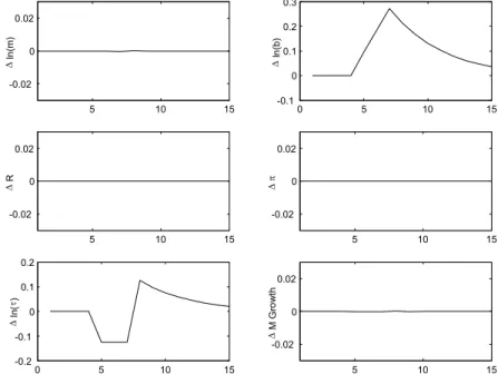
Under an AM/PF and AM/AF specification, figure 11 illustrates the effects of a
4-year switch to an AM/AF regime from an AM/PF regime. Thefigure also shows a
switch back to the AM/PF regime at period 8. The switch from AM/PF to AM/AF causes taxes to fall and then no longer respond to debt. The monetary authority
refuses to allow inflation to revalue the increase in debt and thus, the combination
of policies result in a temporarily explosive path for real debt. Agents continue to 16This characterization of the restrictions ensuring global stability is a simplification designed to
highlight the restrictions with a model where the regimes are persistent. In general, a dynamic model with all locally stationary regimes is neither necessary or sufficient for global stability. Francq and Zakoian (2001) provide an example where the local stationarity of all regimes does not imply global stationarity. Using an AR(2) process where the series increases when switching occurs, a transition matrix resulting in frequent regime changes results in a globally explosive process.
purchase and hold debt, however, because they anticipate a change to a regime that
raises taxes to service and pay off the debt.17
7. Some Empirical Implications
This section derives two empirical implications from the theoretical regime-switching environment. The implications are demonstrated using time series produced by sim-ulating the benchmark model for 100,000 periods. The simulation allows regime to
evolve according to the transition probabilities in (12) and draws (θt, ψt) from their
normal distributions.
7.1. The “Price Puzzle”. The “price puzzle” that emerges from many attempts to identify exogenous shifts in monetary policy is well documented [for example, Sims (1992), Eichenbaum (1992), Hanson (2002)]. It was regarded as a puzzle because a monetary expansion that lowers the nominal interest rate is often followed by lower
inflation, rather than higher inflation, as many theories would predict. Several papers
try to resolve the puzzle by changing identifying assumptions or by expanding the information set on which policy choices are based [for example, Gordon and Leeper (1994), Leeper, Sims, and Zha (1996), Christiano, Eichenbaum, and Evans (1999), Bernanke, Boivin, and Eliasz (2002), Leeper and Roush (2003)].
Another reaction has been that lower inflation following a lower interest rate is not
a puzzle at all. To the extent that firms must borrow to finance wage bills and new
investment, lower interest rates reduce the costs of production and can lead naturally
to lower inflation, at least for some period [Barth and Ramey (2001), Christiano,
Eichenbaum, and Evans (2001)].
As suggested in section 4, a positive correlation between the interest rate and future
inflation is also a natural outcome of the switching model. It appears subtly under
regime 1 (AM/PF) and forcefully under regime 2 (PM/AF). We now show that if
time series data were generated by this setup, one should expect tofind that positive
interest rates innovations predict higher inflation.
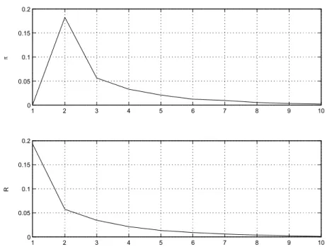
Figure 12 shows the responses of inflation and the nominal interest rate to an
orthogonalized innovation in the nominal rate. Ordering inflation before the interest
rate is consistent with much of the VAR work, which treats inflation as predetermined,
and is also consistent with estimates of the Taylor rule, which regress the nominal
rate on inflation (and potentially other variables). Although the policy disturbances
are i.i.d. and the monetary policy rule is purely contemporaneous, the interest rate 17These results are similar to Woodford (1998), who conducts the same experiment with Ricardian
displays substantial serial correlation. Inflation rises sharply in the short run, and remains above its initial level for 10 periods.
The model’s results are consistent with the Hanson’s (2002) careful analysis. He
finds that the “price puzzle” cannot be solved by the conventional method of adding
commodity prices to the Fed’s information set. And more to the point for the present
work, Hansonfinds that the “puzzle” is more pronounced in the period 1960-1979. But
Favero and Monacelli (2003) identify that period as one where monetary policy was
passive and fiscal policy was active. As figure 5 shows, the model predicts precisely
this outcome when conditioning on PM/AF.
7.2. Surplus-Debt Regressions. A number of authors have computed regressions
of budget surpluses and government debt to draw inferences about the source offiscal
financing [for example, Canzoneri, Cumby, and Diba (2001), Bohn (1998), Janssen,
Nolan, and Thomas (2001)]. Canzoneri, Cumby, and Diba (CCD), for example,
estimate a bivariate VAR with the government surplus and total liabilities.18 Their
figure 3 reports that a positive innovation in the surplus is followed by persistently
lower liabilities and a surplus that is significantly positive for only two periods. They
argue that a Ricardian interpretation of the data is “more plausible” than is a non-Ricardian one, as the increase in the surplus is used to retire debt.
Simulated data from the regime-switching model produce a pattern of correlation
strikingly similar to the top panel of CCD’s figure 3. A positive innovation to the
surplus produces an immediate and persistent decline in liabilities [figure 13].19 Of
course, asfigure 1 makes clear, even conditional on current tax policy being Ricardian,
tax shocks always generate wealth effects and non-Ricardian outcomes.
Our setup is completely straightforward and plausible. Both a reading of Amer-ican tax history over CCD’s sample period and the corroborating formal statistical evidence that Favero and Monacelli (2003) present support the view that monetary
and fiscal policy regimes have switched in a manner that our setup aims to capture.
8. Concluding Remarks
In most countries monetary andfiscal authorities cannot credibly commit to always
follow either active monetary policy and passivefiscal policy or passive monetary
pol-icy and activefiscal policy. If as a consequence, private agents place probability mass
on both kinds of regimes, then something like the regime-switching environment that 18The surpluses is defined to include seigniorage and total liabilities are the sum of net government
debt and the monetary base.
19Given the paucity of independent disturbances in the model and the simple form of the tax rule,
which excludes any contemporaneous response to other variables, in the reverse Choleski ordering– liabilities, surplus–an orthogonalized innovation to the surplus has no predictive value for liabilities.
we model will apply. That environment makes wealth effects–from both monetary and tax policy disturbances–important for determining the impacts of policy.
The implications of this switching setup raise some doubts about two pillars of
recent policy analysis. First, because tax changes have wealth effects, even if the
prevailing regime combines the Taylor principle for monetary policy with taxes that respond strongly to debt, Ricardian equivalence may be a misleading benchmark. Sec-ond, the Taylor principle can actually be destabilizing in the sense that it propagates
disturbances and can increase the variance of aggregate demand and inflation.
There are at least two dimensions along which to extend the current framework. Is it possible for both policy authorities to act passively in one regime, yet have the price level uniquely determined? It is not clear whether the current computational approach can deliver and appropriately characterize a solution with multiple equilibria or sunspots, as Lubik and Schorfheide (2003a) have done for linear models. The
second extension addresses the question: how “big” are the fiscal effects when the
current regime is AM/PF? To address this, we need a carefully calibrated model with frictions, possibly of the kind in the workhorse New Keynesian model extended to include long-term government debt as in Cochrane (2001a). With such a model in hand, we could extract a more complete set of empirical implications. In the New
Keynesian model monetary policy has more conventional macro effects, in addition
AppendixA. Why Linear Methods Fail
This appendix examines the suitability of various linearization approaches to solving the regime-switching model. Our conclusion is that none of these linearization approaches can be expected to give an accurate characterization of the stability of the full non-linear system in all of the cases of interest to us. This conclusion is somewhat surprising, given the nearly linear dynamics of the full system. Essentially, linearized models miss the role of the endogenous expectation error in determining the long-run behavior of the system. Since the qualitative properties of the dynamics are determined by the system’s long-run behavior, these linearized models fail to present an accurate picture of it. In particular, they may fail to classify existence and uniqueness of equilibrium correctly.
To get an intuitive sense of the problem with linearized models, considerfirst a straightforward lineariza-tion around a deterministic steady-state associated with one of the regimes. For the next few paragraphs, we will work with a simplified version of the model, in which seigniorage is identically zero. The government budget identity is therefore
bt= Rt−1bt−1
πt −γ1tb
t−1+g−γ0t−ψt, (17) where(γ0t, γ1t)denote the regime-dependent parameters of the tax rule,(γ0(St ), γ1(St )).
Now define the expectation errorηt = 1 πt/Et−1 h 1 πt i
. Using this definition and the Fisher equation, the government budget identity can be re-written as
bt= µ ηt β −γ1t ¶ bt−1+g−γ0t−ψt. (18)
The linearized version of this equation is
∆bt= µ 1 β −γ1 ¶ ∆bt−1+g−∆γ0t−ψt+ b β∆ηt−b∆γ1t, (19)
where∆b≡bt−b, andbis the steady-state value of real bonds under one of the regimes.
In the single-regime version of the model, the expectation error isi.i.d.and, therefore, the linearized ver-sion accurately captures the stability properties of the model. (See end of appendix C for proof.) However, in the full non-linear regime-switching model, the expectation errorsηt are correlated with futureγ1. Con-sequently,ηtcannot be replaced by1/βin expectations of the form EtQ∞k=1
³η t+k
β −γ1t+k ´
. Accordingly, in general, the long-run properties of the linearized model will be different from those of the full non-linear model, as the long-run behavior is governed by the expected value of such products.2 0
Now consider an alternative linearization approach. Since the equilibrium policy functions in this model appear to be nearly linear, one might imagine that a state-contingent linearization approach would be successful in reproducing the long-run properties of the full system. In this case, at each date we linearize around the steady-state associated with the regime holding at that time. The resulting random-coefficients equation is ∆bt= µ 1 β −γ1t ¶ ∆bt−1+g−γ0t−ψt+ b β∆ηt. (20) 2 0
T his p ossibility preclud es using m any of th e stan dard secon d-order accurate expansion s availab le in the literature. Typ ically, it is an assum p tion of these m eth ods that thefirst-ord er lin earization accu rately determ in es the long-run b ehavior of th e system an d th is assum ption is not n ecessarily satisfied for our m odel [K im , K im , S ch au mb erg, and Sim s (2003), Sch m itt-G roh e an d U rib e (2004)].
Again, the problem will be that, whenη is significant, the long-run dynamics of the random-coefficient models may fail to represent the stability properties of the full system.
To get a sense of the importance of this possibility, we can compare the results of the linearized models to the full non-linear model for special parameter values for which it is possible to solve the full model exactly. Suppose that monetary policy obeys the ruleRt= exp(α0t+α1tπ1t+θt). Using the Fisher equation, and using the definition of the endogenous expectation error, the dynamics for inflation can be written as
b
πt+1=α1tπbt+θt+α0t+ lnβ−bηt+1,
whereˆdenotes the natural log of the variable.
In appendix B, we show how to determine some long-run properties of this difference equation. For certain parameter values it will turn out that imposing stability on the inflation process is sufficient to determine the mapping between inflation and the exogenous shocks. These are the determinate Ricardian equilibria of this model. Having solved forπ, we can then obtain an expression for the endogenous expectation errorη.
Now return to the government budget identity (this time with seigniorage):
bt= µ ηt β −γ1t ¶ bt−1+Υt,t−1, (21) whereΥt,t−1≡ mt−1
πt −mt+gt−ψt. The solution forπimplies that inflation depends only on the current
regimeSt and realization ofθ. Therefore,Υt depends only on current and laggedθt andSt .Appendix C shows that the stability of this equation can be determined becauseηis known.
In Ricardian equilibria, we can compare the results of the full non-linear model with those of the straight-forward linearization around a single steady state. Results are predictably poor and we will not describe them in detail. More interestingly, we can also compare the random-coefficients linearization with the full model. With the random-coefficients model, however, the only qualitative difference between the two models arises in results concerning the stability of the government budget identity: the random-coefficients model may suggest stability when the full model is not stable and vice-versa.
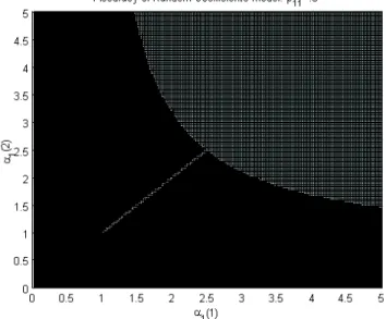
As a baseline, consider the model with γ1(1) = .275and γ1(2) = 0, p11 = p22 = .99, α0(1) = −.5,
α0(2) =.5. With this setting, the two linearization schemes report that the bond dynamics are stable if inflation dynamics are. However, such is not the case in the non-linear system. Figures 14-16 report the results of varyingα1systematically between 1 and 5. The lightly-shaded areas represent regions identified as Ricardian by both linear methods and by the exact solution to the full system. Areas shaded in the middle tone are regions of the parameter space which do not support an equilibrium in the full system, but which are equilibria for the linearized system. Finally, dark regions are areas that, according to the non-linear model, lie outside of the Ricardian space, including non-Ricardian and indeterminate equilibria.
As is apparent fromfigure 14, with the baseline settings there is a substantial region in which the linearized methods fail to capture the long-run behavior of the system, even though the dynamics conditional on regime are nearly linear. Intuitively, these results arise because the regimes are long-lived, while inflation behavior may differ substantially across regimes. Say, for example, that inflation is much higher in regime 1 than in 2. Then, while the system switches from 1 to 2, the inflation rate falls dramatically, generating a large value forη. Moreover, while in regime 2, the inflation rate is persistently and substantially below expectations. The growth rate of debt is therefore higher than the ex ante real interest rate, at the same time that taxes fail to respond to lagged debt. The ultimate effect is that the growth rate of debt is explosive, while the linear model, which does not capture these correlations, suggests that debt is stable.
To gauge the sensitivity of the model to these effects, we varied several parameters of the baseline, including the persistence of the regimes, the standard deviations of the shocks and the intercept terms in the monetary policy rule.2 1 Results of these variations are presented infigures 15-16. Reducing the persistence of
the regimes leads to smaller differences in inflation behavior between regimes. Correspondingly, the forecast errors, on average, are not as large, while also not as informative about future tax policy. Linear methods then are quite successful in tracking the long-term behavior of the system, as shown infigure 15, which increases the transition probability to 70%. Increasing the gap between the intercepts in the two regimes increases the spread in inflation rates across regimes and for similar reasons the performance of linear models becomes commensurately poor. (Figure 16 presents results from a run with the intercepts set at 1 and -1. The region of the parameter space over which the linear model mis-characterizes the long-run behavior of the model is much larger than the corresponding region for the baseline.)
Nevertheless, given our wish to explore the parameter space over fairly broad regions and with relatively persistent regimes, the linearized models are clearly not suitable. With widely separated, persistent regimes, the expected growth rate of debt is significantly affected by much lower-than-expected (or higher-than-expected) inflation. Neither of the linearization approaches matches this feature of the full model, and so cannot match its dynamics in general.
Appendix B. Stability Properties of Random-Coefficient Linear Models
For our purposes, it is sufficient to consider the stability properties of a simple univariate model of the following form:
xt=αt−1(St−1)xt−1+ξt−1+Π(St)ηt,
whereαtfollows anM-state Markov chain,ξtis an exogenous shock process possibly depending on both the state of the Markov chain and onQadditionali.i.d.processesΘandηtis an endogenous expectation error, satisfying the constraintEtηt+1= 0. Let the transition matrix of the Markov chain be given byπ, where
πij=prob(st+1=i|st=j). Finally, the expectationEt is taken with respect to the timetinformation set {xt−j, St−j, ξt−j, ζt−j|j≥0}, whereζ represents a non-fundamental (“sunspot”) shock.
We are interested in the behavior of Etxt+T asT becomes large. Iterating forward on the model shows that Etxt+T =Et ÃTY−1 j=0 αt+j ! xt+Et T X j=1 ÃT−Yj−1 k=0 αt+k+j ! ¡ ξt+j−1+Πηt+j ¢ . This expectation can be calculated explicitly using the following recursion relation:
Et "YT j=0 αt+j|St=k # = M X m=1 Et+1 "TY−1 j=0 αt+j|St+1=l # a(k)·prob(St+1=l|St=k).
Define the matrix ΓbyΓij≡a(j)·prob(St+1=i|St=j) and let the symbol
Et(a(tl)|•)≡ Ã Et " l Y j=0 αt+j|St= 1 # , ..., Et " l Y j=0 αt+j|St=M #! ,
so that dim(Et(a(tl)|•)) = 1×M. With this notation, the previous recursion relation can be written
Et(a (l) t |•) =Et(a (l) t |•)Γ. Accordingly,Et(a (l) t |•) =ωΓ (l)
, whereωis a1xM vector of ones. From this relation, it follows that forj > 1,
2 1
A lterin g the varian ce of thei.i.d.sh ock d oes not have a very dram atic im pact on the p erform an ce of the linear m odel. T herefore, we d o n ot d isp lay a graph for this case.
Et(a (l) t+jξt+j−1|St = m) = M X n=1 prob(St+j−2 = n|St=m)· M X k=1 Et+j−2(ξt+j−1|St+j−1=k, St+j−2=n)·prob(St+j−1=k|St+j−2=n) × M X p=1 Et(a (l) t+j|St+j = p)·prob(St+j−1=k|St+j=p) and therefore Et(a (l) t+jξt+j−1|•) =ωΓ l (πµπj−2), whereµij≡Et+j−2(ξt+j−1|St+j−1=i, St+j−2=j)·prob(St+j−1=i|St+j−2=j). Forj= 1,Et(a (l) t+1ξt|St=m) =ξtωΓ lπ.
Finally, the endogenous expectation errors can be handled as follows. Consider terms of the formd(St)ηt. Then define the basis random variables χj(St) associated with the Markov stateSt, which are defined so thatχj(St) = 1ifSt=jand 0 otherwise.
Projectd(St)ηtonto theχjandΘ, theQadditionali.i.d.processes:
d(St)ηt= M X n=1 anχn(St) + Q X l=1 blΘl+ε,
whereεis uncorrelated with theχj andΘ. Note thatEtat(+l)j|St=mis measurable with respect toSt, so must be expressible as a linear combination of theχj. It follows that
Eta(tl+)j+1Πd(St+j)ηt+j|St=Eta(tl+)j+1Πd(S^t+j)ηt+j|St,
whered(S^t+j)ηt+j≡ PM
n=1anχn(St) +PQl=1blΘl.Ultimately, therefore, we can treat the expectation errors just as we treat theξ, since any dependence on the sunspot shocksζdrops out of the expectations of interest. From here on, let us assume thatΓand πhave M distinct non-zero eigenvalues. With these recursion relations, write Etxt+k=ω Ã Γk(X+ξ/a(St)) + k X j=1 Γk−j(ηπ−1+πµπ−2)πj ! , whereX=diag(x(1)...x(M)).
Now decomposeΓandπinto linear combinations of projectors onto their eigenvectors:Γ=PjM=1λjPj(Γ) andπ=PMj=1φjPj(π). Then the sum over future shocks can be calculated explicitly to arrive at
Etxt+k=ω M X m=1 Pm(Γ) Ã λkm·(X+ξ/a(St)) + M X n=1 µ λkm−φ k n λm−φn ¶ (ηπ−1+πµπ−2)Pn(π) ! .
Therefore, the long-run expected properties ofxare characterized by the number of explosive roots ofΓ.
AppendixC. Solving a Ricardian Model
From the Fisher equation and the monetary policy rule, we have that1/Rt=βEt1/πt+1= exp(−α1tπt− α0t−θt), where θt is i.i.d. Defining ηt+1 =
1/πt+1
Et1/πt+1, we can rewrite these equations in logs as bπt+1 =
α1tπbt+θt+α0t+ lnβ−bηt+1.In this case,bηis not mean-zero, as is apparent from its definition. Therefore, we decomposebηinto its mean and deviations from the mean:bηt+1=ηet+1+Etbηt+1. Because the monetary policy shock isi.i.d., the mean is purely dependent on the Markov stateSt. From here on, letνt(St) =Etbηt+1.
Written in this form, inflation dynamics are of the form described in Appendix B, and, therefore, stability in expectation requires that, for every explosive rootλm,
ωPm(Γ) Ã X+ 2 X n=1 φn ½ θt λm + ηπ −1 λm−φn ¾ Pn(π) ! = 0,
where we have dropped the intercept term from the expression for the sake of convenience. The intercept containsνt, which must be determined later. In any event, the contribution of the intercept only adds a purelySt dependent term to the expression forx(St).
The operatorQm≡P2n=1ξn Pn(π)
λm−φn is invertible, so, assuming that both roots ofΓ(A)are explosive, we
can write 2 X m=1 ωPm(Γ) Ã X+ 2 X n=1 φn θt λm Pn(π) ! ( 2 X n=1 λm−φn φn Pn(π) ) = 0
sinceωη= 0. This leads to the following sequence of implications:
⇒ 2 X m=1 ωPm(Γ) ( X· 2 X n=1 λm−φn φn Pn(π) + 2 X n=1 λm−φn λm θ tPn(π) ) = 0 ⇒ 2 X m=1 ωPm(Γ) 2 X n=1 ½ X 1 φn + 1 λm θt ¾ (λm−φn)Pn(π) = 0 ⇒ 2 X m=1 ωPm(Γ)©X·(π−1λm−I) +θt(I−π/λm)ª= 0 ⇒ω©Γ(A)·X·π−1−X) +θt(I−Γ(A)−1π)ª= 0 Now expand this expression to yield
ω Ã π Ã α1(1)x(1) 0 0 α1(2)x(2) ! π−1−x ! + (1−1/α1(1),1−1/α1(2))θt= 0
Finally, after some further algebra with this expression, we can obtain explicit solutions for the inflation function. In this case, the inflation function is very simple:x(St) =−θt/α1(St).
With the intercept term, we would have obtainedx(St) =−θt/α1(St) + ∆(St), where∆(St)depends on the still-undeterminedEtbηt+1. This term can be determined by imposing the condition thatEtηt+1= 1.
Substituting the result forx(St), we have
βEt{exp (−bπt+1+α1(St)πt+θt+α0(St))}= 1 ⇒βEt ½ exp µ θt+1 α1(St+1)− ∆(St+1) +α1(St)∆(St) +α0(St) ¶¾ = 1
If we assume thatθisN(0, σ), then
Et ½ exp µ θt+1 α1(St+1) ¶ |St+1, St ¾ = exp µ σ 2α1(St+1)2 ¶ and therefore βEt ½ exp µ σ 2α1(St+1)2 − ∆(St+1) +α1(St)∆(St) +α0(St) ¶¾ = 1. This condition, for each initialSt,is sufficient to determine∆(St).
Once the expectations errorsηhave been determined, the long-run properties of the bond dynamics can be derived using a variation of the methods in Appendix B. When steady-state inflation rates are different across regimes, the relevant eigenvalues are those associated with the matrix
³ η(1,1) β −γ1(1) ´ p11 ³ η(1,2) β −γ1(1) ´ p12 ³ η(2,1) β −γ1(2) ´ p21 ³ η(2,2) β −γ1(2) ´ p22
Whenγ1 is independent of regime, however, the law of iterated expectations implies that
Et k Y j=1 µη t+j β −γ1(St+j) ¶ = (1/β−γ1) k .
This result holds when the conditional mean ofγ1 is independent of the initial state. Thus, under these circumstances, the state-contingent linearization scheme will perfectly capture the long-run behavior of the full non-linear system.
AppendixD. Solving the Non-linear Regime-Switching Model
The complete model consists of a system of non-linear expectational difference equations composed of thefirst-order necessary conditions from the representative agent’s optimization problem, constraints, spec-ification of the policy process, and the transversality conditions on real balances and bonds. The solution method, based on Coleman (1991), conjectures candidate decision rules that reduce the system to a set of non-linear expectationalfirst-order difference equations. The solution consists of two funct