HAL Id: hal-02459508
https://hal.archives-ouvertes.fr/hal-02459508
Submitted on 10 Mar 2020
HAL
is a multi-disciplinary open access
archive for the deposit and dissemination of
sci-entific research documents, whether they are
pub-lished or not. The documents may come from
teaching and research institutions in France or
abroad, or from public or private research centers.
L’archive ouverte pluridisciplinaire
HAL
, est
destinée au dépôt et à la diffusion de documents
scientifiques de niveau recherche, publiés ou non,
émanant des établissements d’enseignement et de
recherche français ou étrangers, des laboratoires
publics ou privés.
To cite this version:
Vinh-Loc Dao, Cécile Bothorel, Philippe Lenca. Community structure: A comparative evaluation
of community detection methods.
Network Science, Cambridge Journals, 2020, 8 (1), pp.1-41.
�10.1017/nws.2019.59�. �hal-02459508�
Community Structure: A Comparative Evaluation
of Community Detection Methods
VINH LOC DAO, CECILE BOTHOREL and PHILIPPE LENCA IMT Atlantique,
Lab-STICC CNRS UMR 6285 F-29238, Brest, France
(e-mail:{vinh.dao, cecile.bothorel, philippe.lenca}@imt-atlantique.fr)
Action Editor.Filippo Menczer
Abstract
Discovering community structure in complex networks is a mature field since a tremendous number of community detection methods have been introduced in the literature. Nevertheless, it is still very challenging for practioners to determine which method would be suitable to get insights into the structural information of the networks they study. Many recent efforts have been devoted to investigating various quality scores of the community structure, but the problem of distinguishing between different types of communities is still open. In this paper, we propose a comparative, extensive and empirical study to investigate what types of communities many state-of-the-art and well-known community detection methods are producing. Specifically, we provide comprehensive analyses on computation time, community size distribution, a comparative evaluation of methods according to their optimisation schemes as well as a comparison of their partioning strategy through validation metrics. We process our analyses on a very large corpus of hundreds of networks from five different network categories and propose ways to classify community detection methods, helping a potential user to navigate the complex landscape of community detection.
Keywords. community detection, community structure, comparative analysis, empirical analysis, computation time, community size, structural quality function, validation metric, decision-making assistance for practioners
Statement of conflict of interest.Vinh Loc DAO, C´ecile BOTHOREL and Philippe LENCA have nothing to disclose.
Contents
1 Introduction 2
2 Community detection methods and dataset 4
2.1 Community detection methods 4
2.2 Experimental dataset 7
3 Preliminary analysis of community detection methods 10
3.2 Analysis on community size distribution 15
3.3 Similarity based on community size distribution 25
4 Quality profiling of community detection methods 30
4.1 Community quality metrics 30
4.2 Co-performance index 34
5 Partitioning strategy comparison 37
5.1 Validation metrics 37 5.2 Empirical results 40 6 Related work 41 7 Conclusion 44 References 45 1 Introduction
In network science,community detection(sometimes calledgraph clustering) is one of the fundamental challenges to discovering the structure of networks on the mesoscopic level. However, it is an ill-defined problem. According to Arifinet al.(Arifinet al., 2017),“it does not have clear goals, solution paths or expected solution”. There is no universal defi-nition or closed form formula of what kind of objects one should be looking for (Fortunato & Hric, 2016), and consequently there is no golden standard to assess the quality of a community structure and the performance of a community detection algorithm.
The most frequently found definition of community in the network science literature is derived from the mechanism of connection preference. It implies thata community is a group of nodes (a subgraph) in a graph where there must be more edges (denser) connect-ing them together than edges connectconnect-ing the community with the rest of the graph(Radicchi
et al., 2004; Fortunato, 2010). Newman defines a community as a“group of vertices with a higher-than-average density of edges connecting them”(Newman, 2006b). Depending on the context, a community may be called acluster, amodule, aclassor amodular group. This is the most basic definition that sets the fundamental requirement for most of its derivative definitions. Many different variations of community could be found in (Wasser-man, 1994), for instance,LS-set, which is a set of nodes in a network such that each of its proper subsets has more ties to its complement within the set than outside; ork-core, which is a subgraph in which each node is adjacent to at least a minimum numberkof the other nodes in the subgraph. However, in recent developments of community detection algorithms, there is no consensus of the quantity of edges in reality that could be considered as“many”. Communities are just algorithmically defined, i.e. they are final products of the algorithm without any precise a priori definition (Fortunato, 2010).
In practice, there are even more constraints, which are sometimes not explicitly ex-pressed, than which appeared in the announcement of the problem. If one only looks for a partition of a graph that maximizes the number of internal edges and minimizes the number of external edges, then the graph itself can be considered as a big community with no external connection. Another solution is to leave the node having the smallest degree of a graph in one community, and all other nodes in another community. This solution could also maximize the ratio between external and internal edges. However, these monotonous
solutions do not seem to seduce most (if not all) analysts considering using a community detection algorithm to detect communities. In fact, it is preferable to cluster a network into groups of relatively similar size (Newman, 2010). This means that somehow, the relative size of communities is significant but this notion of size has not been explicitly announced. Besides, there are many other criteria that could be mentioned such as community complete mutuality, reachability, vertex degree distribution and the comparison of internal versus external cohesion (Wasserman, 1994; Fortunato, 2010). There exists a subtle compromise between adding into a community new vertices—along with their edges— and conserv-ing the common property that defines the group. In fact, different community detection methods have different ways to define what defines the groups and how to consider those constraints or not. They produce different community structures. The following are the main reasons that could lead to these disagreements between detection methods:
• Different algorithms may implement different meanings of the notion of community. • When two algorithms define the same concept of community, it may also mathe-matically and algorithmically be formalized in different ways (same objective but different objective functions) and hence leads us to different results.
• Even when two algorithms have exactly the same objective function, the algorithmic mechanism they employ to find communities also decides what they are going to find, especially in heuristic searching approaches.
• Initial configuration is also another important factor that affects the final result of an algorithm, many community detection methods are not deterministic.
• Each method may include a consideration between obtaining an optimized solution and providing reasonable performances (in terms of calculation time, memory con-sumption, etc.). This trade-off may be considered differently across the methods. • Some algorithms are variable according to input data and will prove more or less
efficient on some kinds of inputs than on others.
• Variations due to implementation factors could also impact the final result of an algorithm.
• Finally, in some algorithms, there are tie-break situations where they have to choose randomly without any factor related to their final objectives. It may also significantly affect the result that one would get if the tie-break problems have been resolved in a different way.
Due to the many reasons stated above, choosing the community detection method that corresponds well to a particular scenario or to an expectation of quality is not straightfor-ward. This paper is not the first effort as a guide for choosing community detection meth-ods. For the same purpose, readers can also refer to (Fortunato & Hric, 2016), (Ghasemian
et al., 2018), (Jebabli et al., 2015), and (Jebabli et al., 2018). The difference with ex-isting work is that we provide an exhaustive empirical evaluation on many state-of-the-art methods, using a large network dataset (more than 100 different real networks, of which only a few are synthetic) and using popular quality scoring functions of structural characteristics of communities. Hence, we are able to disclose a performance review of many different methods based solely on empirical experiments and measurements that help network practitioners to reveal the functionality of each method, and behaviours that they could exhibit in real world networks, independently of theoretical mechanisms. The
objective of this work does not differ from existing work in the literature. It does not aim to bring readers an innovative factor in the community detection problem nor discuss every related challenging point of the community detection problem. However it provides an evaluation as well as an approach to examine community detection algorithms. This evaluation is very useful for network practitioners to obtain a quick notion of community structure quality before actually applying a method to their concrete dataset. These notions of quality are expected to guide users to appropriate choices of methods according to their quality criteria.
The paper is organized as follows: Section 2 introduces some popular and state-of-the-art community detection methods that will be analyzed in this paper as well as the benchmark-ing dataset employed in our experiments. Then, Section 3 presents analyses of the most essential aspects of community detection performance including computation time, com-munity size distribution as well as numbers of detected communities by each method. In Section 4, we address different structural quality aspects of community structures. This is followed by a comparative evaluation using many popular clustering validation metrics in Section 5, which are widely used in the context of community detection. The Sections 3 to 5 are independent. They bring complementary material and criteria to describe the quality of community structures and compare the different methods from different perspectives. Each section is detailed, making this article a little long, but they end with a summary that allows readers to get an overview and provide them with the necessary key lessons to be learned. Finally, we present some close results of related work that can be found in the literature in Section 6 and conclude our study with some discussions and recommendations in Section 7.
2 Community detection methods and dataset
2.1 Community detection methods
We present, in this section, some popular community detection methods that have been widely used and discussed in the literature. Note that in recent years, there are a large number of innovative methods which have been proposed to solve either generic or specific cases. However, an empirical and exhaustive analysis of all methods would be impracti-cal, even unrealizable. To the best of our knowledge, we are trying to include the most important and representative methods among the community detection approaches.
There are many possible theoretical taxonomies for community detection methods, de-pending on the final objective of each categorization. For instance, one could classify methods according to differences in searching mechanisms, objective functions, assump-tions about the structure to be found, expected qualities, hypothesis models, or even the theoretical model employed, etc. Moreover, what makes the problem trickier is that many methods are not just some simple algorithms to resolve a specific problem, but instead are combinations of many different approaches in order to leverage as much algorithmic power as possible from each one. There is not a consensus on how different methods are similar and how they can be classified into different families whose functionality can be resumed in some simple words. Porter et al. use centrality based, local techniques, modularity
In (Fortunato, 2010; Fortunato & Hric, 2016), the authors group community detection methods into traditional data clustering methods, divisive algorithms, modularity-based methods, spectral algorithms, dynamic algorithms and methods based on statistical infer-ence. Coscia et al.classify community discovering into feature distance based, internal density, bridge detection, diffusion process, closeness based, structural pattern based, link clustering, meta clustering (Cosciaet al., 2011). In a context of Social Media, Papadopulos
et al. compare methods in substructure detection, vertex clustering, community quality optimization, divisive and model-based approaches (Papadopoulos et al., 2011). Bohlin
et al. aggregate different approaches into three principle classes representing different network models: null models, block models and flow models (Bohlinet al., 2014). Schaub
et al.classify methods into four perspectives: cut based, clustering internal density based, stochastic equivalent based and dynamic based showing four different facets of community structure (Schaubet al., 2017). Finally, Ghasemianet al.adopt an experimental classifica-tion (Ghasemian et al., 2018) as well as group community detection methods in distinct families based on their outputs on many real-world networks using a validation metric (a topic we will address in Section 5.1).
In the following sections, we choose to classify community detection methods accord-ing to different theoretical approaches includaccord-ing edge removal, modularity optimization, spectral partitioning, dynamic process and statistical inference. Although every theoretical taxonomy may be questionable, this categorization is expected to support the empirical analyses in the next sessions to verify whether theoretical and conceptual closeness could engender quality closeness in practice.
2.1.1 Edge removal based methods
Edge betweenness (GN) (Newman & Girvan, 2004) detects communities by removing edges progressively according to their betweenness centrality scores. This method is based on the intuition that dense areas of a graph are loosely connected by a few edges that are located in the shortest paths between pairs of nodes. Removing these edges would reveal densely connected communities.
Edge clustering coefficient(RCCLP) (Radicchiet al., 2004) suggests replacing the edge betweenness centrality of Girvan-Newman’s method by an edge clustering coefficient, which requires less computation time and hence reduces the complexity. In this paper, we analyze two configurations of this method corresponding to triangular (g=3 denoted byRCCLP-3) and quadrangular (g=4 denoted byRCCLP-4) versions.
2.1.2 Modularity optimization methods
Greedy optimization (CNM) (Clauset et al., 2004) greedily maximizes the modularity functionQby aggregating iteratively connected communities which induces a maximum increase or minimum decrease in modularity∆Q.
Louvain method(Blondelet al., 2008) adopts a two-step agglomerative process similar to the greedy optimization method. However, in each iteration of the first step, it allows nodes to move between communities until no additional gain in modularity can be obtained with these local switches. Then, a new graph whose vertices are the communities resulting from
the first step is built and the process is repeated on the new graph to reduce computation time, leading to a hierarchical clustering.
Spectral method(SN) (Newman, 2006a) reformulates the idea of maximizing modularity as a spectral partitioning problem by constructing amodularity matrixand using its leading eigenvector to spectrally partition networks into sub-networks. The community structure is identified using the eigenvectors of this matrix. Eigenvectors are used to project each node into low-dimensional node vectors, and the community structure is identified through clustering the node vectors (e.g. with the k-means clustering method).
2.1.3 Dynamic process based methods
Walktrap(Pons & Latapy, 2005) defines a pairwisedynamic distancebetween nodes and then applies traditional hierarchical clustering to detect community structure. The distance between two nodes is defined in terms of a random walk process. The basic idea is that if two nodes are in the same community, they tend to”see”other nodes in the same way, i.e. the probability of getting to a third node through a random walk should not be very different for these two nodes, with higher distance for nodes belonging to other communities.
Infomod(Rosvall & Bergstrom, 2007) uses an information theoretic model where a sig-nalertries to send the structure of a network over a limited capacity transmission channel to areceiver. The network must be encoded in community structure in a way that minimizes the transferred information and the information loss.
Infomap(Rosvallet al., 2009) represents networks by a two-level structure description. Analogically, each node in a network is encrypted by a unique codeword composed of two parts: a prefix representing the community to which it belongs and a suffix representing the local code. Detecting community structure becomes equivalent to searching for the coding rule to minimize the average code length describing random walks on the network.
2.1.4 Statistical inference based methods
Stochastic Block Model(SBM) (Rioloet al., 2017). The Stochastic Block Model was introduced by Hollandet al.(Hollandet al., 1983). Here we use the implementation by Rioloet al.which uses a Monte Carlo sampling scheme to maximize a Bayesian posterior probability distribution over possible divisions of the network into communities. This probability implies an expected network model to be fitted from the observed network data. In this block model variant, the authors employ a new prior on the number of communities based on a queueing-type mechanism to calculate posterior probability. We analyze, in the following sections, both traditionalSBMand thedegree-correctedversionDCSBM, which had been proven to perform better in practice.
Order statistics local optimization(OSLOM) (Lancichinettiet al., 2011) measures the statistical significance of a community by calculating the probability of finding a similar one in a null model. Following this concept, nodes are gradually aggregated into commu-nities to find significant commucommu-nities. Then nodes are considered to be swapped between communities in order to increase significance level.
2.1.5 Other methods
Spin glass model(RB) (Reichardt & Bornholdt, 2006) is a method relying on an analogy between the statistical mechanics of complex networks and physical spin glass models. It finds communities by fitting the ground state of a spin glass model. Instead of favoring only intra-community edges and penalizing inter-community edges like the traditional modularity measure, this model also favors inter-community non edges and penalizes intra-community non-edges.
Label propagation(LPA) (Raghavan et al., 2007) exploits the topology of networks to infer community structure. It is closely related to the context of message passing paradigms or epidemic spreading. The principled idea of this method is based on the concept that nodes should belong to the community of most of their neighbors. Hence, they gradually update their memberships according to their incident nodes.
Speaker-listener label propagation(SLPA) by Xie and Szymanski (Xie & Szymanski, 2012) modifies the propagation mechanism above by a new label update strategy. Also, instead of keeping only hard membership information, each node is equipped by a mem-ory to contain the labels that it receives. Then, in the update phase, nodes transmit the membership to their neighbors according to the membership frequency in the memories.
Mixing global and local information(Conclude) (Meoet al., 2014) combines a dynamic distance with a modularity optimization process to identify community structure. Firstly, the authors define a new pairwise proximity function using random and non backtracking walks of finite length to determine distances between vertices. Then, the multi-level modu-larity optimization strategy ofLouvainmethod (Blondelet al., 2008) is combined with the defined distance to find community structure.
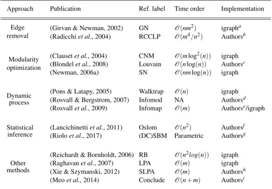
Table 1 summarizes the methods presented previously, grouped by different approaches. Since community detection is receiving more and more attention in the network science community, there is a huge volume of work that has been published in recent years to evaluate different methods including both theoretical and empirical approaches. However, there is no formal and quantitative definition of community that is explicitly implemented inside algorithms. Therefore it is challenging to distinguish the topological differences of community structures using different methods, even when the associated concepts are quite theoretically discernible. Additionally, it is still not clear whether proximity in the assumption of community concept will engender a structural similarity of communities that could be detected. Our comparative analysis in the next sections will try to address these questions in more detail.
2.2 Experimental dataset
In this section, we describe some statistical properties of networks that will be included in the following analysis. Available biological networks that have been published and analyzed widely are relatively small in comparison to the other networks of the other families. Besides, due to the complexity of the analysis process, we limit the domains of interest to 5 categories which are commonly researched and where numerous networks are available. We introduce a 6th category with various types of networks, each of which
Table 1: Community detection methods involved in the study.
Approach Publication Ref. label Time order Implementation
Edge removal
(Girvan & Newman, 2002) GN O(nm2) igrapha (Radicchiet al., 2004) RCCLP O(m4/n2) Authorsb
Modularity optimization
(Clausetet al., 2004) CNM O(mlog2(n)) igraph (Blondelet al., 2008) Louvain O(nlog(n)) Authorsc (Newman, 2006a) SN O(nmlog(n)) igraph
Dynamic process
(Pons & Latapy, 2005) Walktrap O(n) igraph (Rosvall & Bergstrom, 2007) Infomod NA Authorsd (Rosvallet al., 2009) Infomap O(m) Authorse/igraph
Statistical inference
(Lancichinettiet al., 2011) Oslom O(n2) Authorsf (Rioloet al., 2017) (DC)SBM Parametric Authorsg
Other methods
(Reichardt & Bornholdt, 2006) RB O(n2log(n)) igraph (Raghavanet al., 2007) LPA O(m) igraph (Xie & Szymanski, 2012) SLPA O(m) Authorsh (Meoet al., 2014) Conclude O(n+m) Authorsi a Published athttp://igraph.org/ b Published athttp://homes.sice.indiana.edu/filiradi/resources.html c Published athttps://sourceforge.net/projects/louvain/ d Published at http://www.tp.umu.se/~rosvall/code.html e Published athttp://www.mapequation.org/ f Published athttp://www.oslom.org/ g Published at http://www-personal.umich.edu/~mejn/ h Published athttps://sites.google.com/site/communitydetectionslpa/ i Published athttp://www.emilio.ferrara.name/code/conclude/
is under-represented, such as ecological networks for example. In this study, we consider 108 different networks, which is relatively large in comparison to many other studies. Many notable related works where some of these networks are also employed could be mentioned for quick reference: Ormanet al.use 6 networks to evaluate the structure of communities discovered by several detection techniques (Ormanet al., 2012); Lancichinettiet al.use 15 networks to characterize structural communities (Lancichinettiet al., 2010); Hricet al.
use 16 networks to reveal differences between structural communities and ground truth (Hricet al., 2014); Leskovecet al.use over 100 networks to analyze network community profile (Leskovecet al., 2008) and 230 networks to evaluate the goodness of ground-truth communities in social networks. Within this number, 225 samples of the Ning online social networking platform networks1are aggregated (Yang & Leskovec, 2013). Let us mention, finally, the related work by Ghasemian et al. which has introduced the large
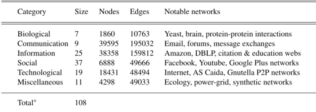
Table 2: A summary of network dataset used in this analysis where “Size” is the number of networks analyzed in each category, “Nodes” and “Edges” indicate the average number of nodes and edges of networks in each category respectively. ∗The last row shows the total number of networks in the whole dataset. This dataset is collected from several sources including: http://networkrepository.com(Rossi & Ahmed, 2015),http: //konect.uni-koblenz.de(Jerome, 2013),http://snap.stanford.edu(Leskovec & Krevl, 2014)
.
Category Size Nodes Edges Notable networks
Biological 7 1860 10763 Yeast, brain, protein-protein interactions Communication 9 39595 195032 Email, forums, message exchanges Information 25 38358 159812 Amazon, DBLP, citation & education webs Social 37 6888 49666 Facebook, Youtube, Google Plus networks Technological 19 18431 48494 Internet, AS Caida, Gnutella P2P networks Miscellaneous 11 4298 49033 Ecology, power-grid, synthetic networks
Total∗ 108
CommunityFitNet corpus2containing 572 real-world networks. Table 2 summarizes the
composition of networks that have been analyzed in this section.
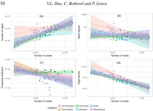
Some notable structural characteristics of networks in the dataset are illustrated in Fig-ure 1. It is noticeable that apart from biological networks which are relatively small, the other classes cover quite a wide range of numbers of nodes, edges, mean degree, clustering coefficient and edge density. Since real world networks are relatively sparse, the number of edges increases linearly according to the number of nodes and consequently, the edge densities decrease linearly by the number of nodes (since the number of possible connections increases quadratically by the number of nodes in a community). This sparsity property can easily be seen in Figure 1(a,d). Specifically, the number of edges increases linearly according to the number of nodes with equivalent rates among different network categories as can be deduced from the gradients of the linear estimates. From Figure 1(b), it can be seen that the average degree of the networks in the dataset varies principally between 1 and 100 edges per node except for 2 communication networks. Also, the majority of networks have an average degree from 10 to 20 connections. From a global point of view, networks in the dataset have a quite strong modular quality since most of them have relatively high clustering coefficients as shown in Figure 1(c).
(a) (b)
(c) (d)
Fig. 1: From left to right, top to bottom, we illustrate structural characteristics of the 108 networks: (a) Number of edges as a function of the number of nodes, (b) Mean degreehki as a function of the number of nodes, (c) Clustering coefficient according to the number of nodes, (d) Edge density as a function of the number of nodes. The colored backgrounds represent the 95% confidence intervals of the relations estimated from the dataset using a linear regression model for the corresponding variables in each network category.
3 Preliminary analysis of community detection methods
3.1 Computation time performance
Since computation time is a crucial factor to be considered in the selection of an algorithm, it is worth analyzing experimental performances to see how different community detection methods accomplish their task in real-world networks. We tested the official implemen-tations of community detection methods introduced in Table 1 on the dataset collection presented in Table 2. The implementations are provided officially either by their authors or by popular network analysis libraries which can be easily accessed by a large public.
We ran the implementations stated above to identify community structures on all the networks in the dataset. We measured the time needed for each implementation to compute each partition on each network. The default parameters configured by the implementa-tions remained unchanged during the test. The calculaimplementa-tions were executed on a server equipped by an Intel Xeon CPU E5-2650 with 32 cores of 2.60 GHz and a memory capacity of approximately 100 GBytes. However, due to the high complexity of some methods, only processes that finish within a practical time limit (less than 4 hours) are taken into account. However, for a reference purpose, we let some longer computations continue. For exampleConcludemethod took approximately 9 days to identify community structures on a network of 300 thousand vertices and 1 million edges;GNmethod did not
finish its calculation for networks of more than 4 thousand nodes and 40 thousand edges within 2 days. Consequently, the experiments that theoretically require too much time are neglected in the test. It is also worth noting that the calculations of communities on large-scale networks are also restrained by limited memory. Thus, calculations that should be finished within 4 hours but required too much memory cannot be shown here either. We repeat the calculations 5 times for each pair graph/method to reduce the fluctuation impact. Eliminating all the cases that do not satisfy our requirements, the final successful rate (number of partitions identified over the number of possible tests) ended at around 44.72%, mainly because of time/memory overflow.
1e-03 1e-02 1e-01 1e+00 1e+01 1e+02 1e+03 1e+04 1e+05 1e+06
1e+01 1e+02 1e+03 1e+04 1e+05 4e+05
Number of vertices
Time (in seconds)
1e-03 1e-02 1e-01 1e+00 1e+01 1e+02 1e+03 1e+04 1e+05 1e+06
1e+01 1e+02 1e+03 1e+04 1e+05 4e+05
Number of edges
Time (in seconds)
Method GN RCCLP-3 RCCLP-4 Theoretical GN Theoretical RCCLP
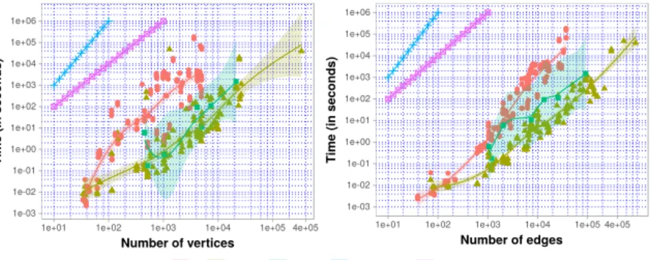
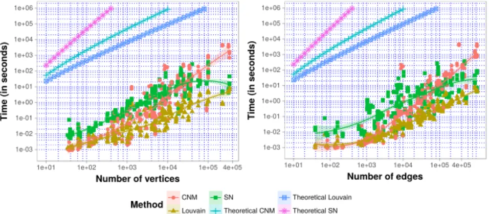
Fig. 2: The execution time needed by GN, RCCLP-3 and RCCLP-4 methods to identify community structures on networks of the dataset.
In the following figures (from Figure 2 to Figure 7) that illustrate the analyses of ex-perimental time consumption, some conventions are commonly used. Points in the figures correspond to separated executions that have been measured. The solid lines with the same colors are estimated relations between computation time and network size (number of vertices and number of edges), using a local regression model (Cleveland, 1979). The dark colored backgrounds around the regression curves represent 95% confidence intervals of the model parameters. Besides, for reference purposes, we also showtheoreticalexecution time (i.e. in the worst case, in terms of number of calculations needed) for each algorithm. In our estimates, we plot this theoretical execution time by assigningn=m, as from the analysis of structural characteristics of the dataset shown above in Figure 1(a), most net-works are sparse, i.e. the number of edges (m) increases linearly with the number of nodes (n). For simplicity of illustration, we grouped our results according to our classification (Table 1).
The first group of methods consists of centrality detection techniques to identify com-munity structure. As we can see in Figure 2, theGN method cannot be accomplished in our test for networks of more than 4 thousand nodes or 30 thousand edges. The outcome is quite reasonable since the theoretical estimation for this method is O(nm2), which
grows quickly with the network size. It should be remembered that the primary goal of the RCCLPmethod is to reduce the time complexity of theGN method. We can easily observe that this objective is achieved since theRCCLP-3reduces by an order of around
103times for graphs of 3 hundred nodes.RCCLP-3can function well with graphs up to millions of edges. However, when we used the same test withRCCLP-4, the method rarely reached its terminus for large graphs as well as small graphs. As we can see in the figure, there are few dots at either side. The reason is that there are not many (they may even be absent) 4-step close paths on real world networks. As it is not very probable that such structures exist in small graphs, finding them in large graphs also requires a huge amount of time,RCCLP-4shows a poor performance in our tests. Therefore, this configuration of the method is not recommended, as versions withg>4 would logically perform poorly. It is also worth noticing thatRCCLP-3andRCCLP-4are extremely memory consuming and are not suitable for limited resource devices. Finally, theoretical and practical time seem to find a consensus as the increments of time according to network size are quite consistent in the three cases.
1e-03 1e-02 1e-01 1e+00 1e+01 1e+02 1e+03 1e+04 1e+05 1e+06
1e+01 1e+02 1e+03 1e+04 1e+05 4e+05
Number of vertices
Time (in seconds)
1e-03 1e-02 1e-01 1e+00 1e+01 1e+02 1e+03 1e+04 1e+05 1e+06
1e+01 1e+02 1e+03 1e+04 1e+05 4e+05
Number of edges
Time (in seconds)
Method CNMLouvain SNTheoretical CNM Theoretical LouvainTheoretical SN
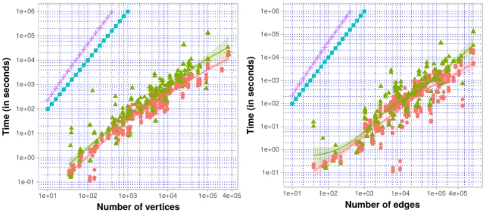
Fig. 3: The execution time needed by CNM, Louvain and SN methods to identify community structures on networks of the dataset.
The next group includes methods using modularity optimization processes whose exper-imental measures are shown in Figure 3. Practically, the three methods in this family re-quire a reasonable time for calculating community structures. The longest experiment took less than 2 hours for a graph of 1 million edges. TheLouvainmethod is the fastest in this group; its computation increases approximately in linear time. It took only 9 seconds for the largest graph. Among the three methods, the optimization using the spectral approach is the most expensive. However, all three methods perform better than the methods in the edge removal group previously stated. The experimental results also verify theoretical estimates concerning the complexity of these methods.
Similarly to the two previous groups, the computation time needed by methods in the dynamic process group is illustrated in Figure 4. In terms of time consumption, this group performs better with respect to the first group, but generally worse than the modularity optimization group (except for theWalktrapmethod for small and average size graphs). Among these three methods,Infomod generally requires more calculation time than the others. At the same time,WalktrapandInfomapwork asymptotically equally well with a slightly better rendition forWalktrapin small and average size graphs.
1e-03 1e-02 1e-01 1e+00 1e+01 1e+02 1e+03 1e+04 1e+05
1e+01 1e+02 1e+03 1e+04 1e+05 4e+05
Number of vertices
Time (in seconds)
1e-03 1e-02 1e-01 1e+00 1e+01 1e+02 1e+03 1e+04 1e+05
1e+01 1e+02 1e+03 1e+04 1e+05 4e+05
Number of edges
Time (in seconds)
Method Infomap Infomod Walktrap Theoretical Walktrap & Infomap
Fig. 4: The execution time needed by Infomap, Infomod and Walktrap methods to identify community structures on networks of the dataset.
1e-01 1e+00 1e+01 1e+02 1e+03 1e+04 1e+05 1e+06
1e+01 1e+02 1e+03 1e+04 1e+05 4e+05
Number of vertices
Time (in seconds)
1e-01 1e+00 1e+01 1e+02 1e+03 1e+04 1e+05 1e+06
1e+01 1e+02 1e+03 1e+04 1e+05 4e+05
Number of edges
Time (in seconds)
Method DCSBM Oslom Theoretical Oslom Theoretical DCSBM
Fig. 5: The execution time needed by DCSBM and Oslom methods to identify community structures on networks of the dataset.
The same analyses for methods in the two final groups are shown in Figure 5 and Fig-ure 6. We can easily see thatDCSBMandOslomhave practically identical performances in terms of time consumption,DCSBMbeing slightly better. In the last group, the results are quite different between different methods. The label propagation methodLPAshows a clear distinctive curve indicating its out-performance compared with the other methods. Besides,SLPAworks quite well, but not as fast asLPAalthough it employs some additional techniques to reduce the number of necessary calculations (Xie & Szymanski, 2012). This difference in performance is due to the more complicated mechanism thatSLPAuses in comparison toLPA. It is due to the fact thatSLPAmanages dedicated memories for all the nodes to stock the membership information and update it regularly. Therefore, despite the improvement of 5 to 10 times in the label update strategy, the global performance cannot surpass that ofLPAmethod. In terms of scalability,LPAandSLPAseem to exhibit the same behavior which is almost linear for small and medium graphs but increases in
1e-03 1e-02 1e-01 1e+00 1e+01 1e+02 1e+03 1e+04 1e+05 1e+06
1e+01 1e+02 1e+03 1e+04 1e+05 4e+05
Number of vertices
Time (in seconds)
1e-03 1e-02 1e-01 1e+00 1e+01 1e+02 1e+03 1e+04 1e+05 1e+06
1e+01 1e+02 1e+03 1e+04 1e+05 4e+05
Number of edges
Time (in seconds)
Method RBLPA SLPAConclude Theoretical RBTheoretical LPA, SLPA & Conclude
Fig. 6: The execution time needed by RB, LPA, SLPA and Conclude methods to identify community structures on networks of the dataset.
large graphs. The spin glass modelRBmanifests a better than expected presentation with an undeviating linear augmentation. The only unexpected behavior is spotted inConclude
method, as when the size of input graphs exceeds some thousands, the required time has been inflated by a factor ofn, making it very demanding for large graphs.
1e-03 1e-02 1e-01 1e+00 1e+01 1e+02 1e+03 1e+04 1e+05 1e+06
1e+02 1e+03 1e+04 1e+05 4e+05
Number of vertices
Time (in seconds)
1e-03 1e-02 1e-01 1e+00 1e+01 1e+02 1e+03 1e+04 1e+05
1e+02 1e+03 1e+04 1e+05 4e+05
Number of edges
Time (in seconds)
method GN RCCLP-3 RCCLP-4 CNM Louvain SN Infomap Infomod Walktrap DCSBM Oslom RB LPA SLPA Conclude
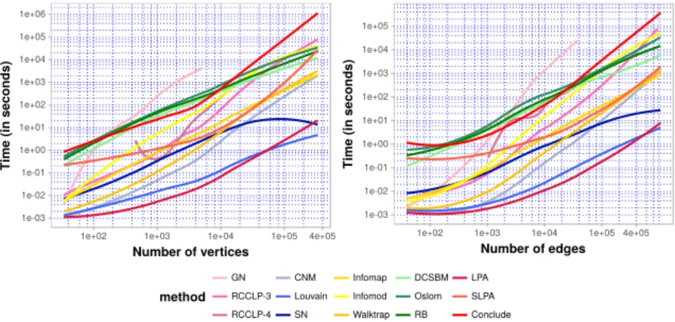
Fig. 7: The estimated execution time needed for each method to identify community structures on networks of the dataset using a local regression model. Methods of the same theoretical family (in the same group) are represented by similar colors.
Finally, we aggregate all the results into a common illustration as shown in Figure 7. At the same time, for more convenient observation, we remove all the points corresponding to each experiment and keep only the regression curves, which are the execution time estimates as a function of the number of vertices on the left side and similarly on the right side for the number of edges. At first sight, it is easy to see that except forGN, the necessary execution time for all other methods is limited in a range that increases polynomially with the network size, which accurately reflects theoretical estimates. This
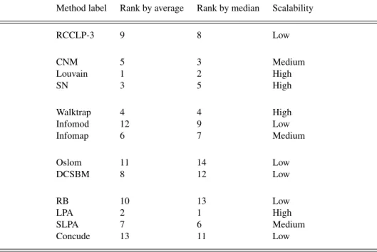
Table 3: Ranking of analyzed methods according to the amount of time consumed, to identify community structures on networks of the dataset.
Method label Rank by average Rank by median Scalability
RCCLP-3 9 8 Low CNM 5 3 Medium Louvain 1 2 High SN 3 5 High Walktrap 4 4 High Infomod 12 9 Low Infomap 6 7 Medium Oslom 11 14 Low DCSBM 8 12 Low RB 10 13 Low LPA 2 1 High SLPA 7 6 Medium Concude 13 11 Low
range is upper-bounded by Conclude/Oslomand lower-bounded byLPA, corresponding to the worst and the best tested method(s) respectively. Another important fact which can be deduced from this figure is that, for most real world networks in the range up to 1 million edges, choosing a fast detection method could economize an order of 103times to 105times the calculation effort. This is an important element to be considered where time consumption is a serious problem.
We demonstrate in Table 3 the ranking of these methods according to our tests for reference purposes.GNandRCCLP-4are not involved in this ranking since they failed to accomplish their tasks in large graphs, which also means they are the most time-consuming methods within the methods that we analyzed. We show both the rankings according to the average and the median of time. Since the average-time ranking is heavily affected by the measurements on large graphs, the methods that were successful in discovering communities on very large graphs are ranked lower than methods that were not able to do so. In these cases, the median ranking is more accurate and reflects therefore the relative performance on small and medium graphs. For large graphs, we recommend using the average ranking.
3.2 Analysis on community size distribution
After these performance considerations, we focus on the nature of the results produced, i.e. the communities themselves. The number of latent communities that should be in-duced from a given network is one of the major questions in community detection context
(Fortunato & Hric, 2016), (Rioloet al., 2017). It is equivalent to the subject of the expected number of clusters in a classical clustering problem. Observing the number of communities reveals useful information about the mesoscopic structure of a network. The variation of the number of communities in a network involves different levels of resolutions. An analogous way to describe the concept of resolution is the distance from an object that we prefer in order to contemplate it. The closer you get to an object, the greater the detail of its micro-structures that can be perceived, while, at the same time, information about the global organization tends to be less clear. Although several multi-resolution approaches (Lambiotte, 2010; Pons & Latapy, 2011) incorporate resolution parameters into their solutions providing more flexible mechanisms and different modular scales of networks, it is not always obvious to regulate these parameters appropriately without ad-hoc cases. The inclusion of multi-resolution parameters, of course, widens the possibility of understanding networks, but at the expense of automation convenience, that is sometimes required in clustering problems.
In this section, we compare, once again, the previously mentioned methods but this time according to their resolution abilities. We use the same dataset collection and again we keep all default configurations of the implementations unchanged to ensure the consistency of future results. From the previous analyses, some modifications will be applied to our testing process as follows:
1. From the observation of the network size distribution in Figure 1(a), as well as the previous computation time analyses, the linear relation between number of vertices and number of edges of networks in our corpus becomes clear. As a consequence, it will be redundant to address the relation of dependent variables in respect of these two latter predictors. Therefore, only analyses according to the number of vertices will be rendered.
2. In the case of the community detection problem, showing only the numbers of com-munities discovered would not always be enough. If we assume that community size in an arbitrary network exhibiting a negative power law distribution (as shown for example in (Clausetet al., 2004)), it means that the number of communities depends heavily on the number of tiny communities. Therefore, we propose to observe the distribution of community size to discern the differences between methods which could not be recognized by seeing solely the number of blocks.
3. Due to the huge number of calculations required and a limited hardware resource, discovering processes in the last section were interrupted unless they could be fin-ished in a few hours. Here, some more efforts have been made, when a method is supposed to be finished in a reasonable amount of time (a few days).
For a given network in the dataset, we applied all of the methods presented, to identify the set of communities predicted by each one and then measured their volumes. Similarly, to the previous section, for simplicity of observation, we group methods by different fam-ilies depending on their approaches. We illustrate the results in Figures 8 to 12 by using some conventions as follows:
Conventions for Figures 8 to Figure 12
1. A figure (denoteda) at the top contains three following sub-figures:
(a) The central figure (a1) shows a scatter plot of the distribution of community size. The solid lines in the figure represent the estimated average commu-nity size using a local regression model (Cleveland, 1979). Dark colored backgrounds around the lines are 95% confidence intervals of the estimates. (b) The top figure (a2) exhibits marginal density distributions of communities found in each range of network sizes. They are rendered by a Gaussian kernel estimator.
(c) The right hand figure(a3) illustrates another type of marginal density distri-bution of communities, as a function of their sizes. They are also rendered by a Gaussian kernel estimator.
(d) The axes of marginal figures are the same as the axes of the corresponding central figure. We simply omit them for ease of representation.
2. A figure on the bottom (denotedb) presents the number of communities as a function of network size (i.e. their number of vertices) as well as the estimated relation between these variables using the regression model stated above. Dark colored backgrounds around the lines show 95% confidence intervals of the estimate relations.
3.2.1 Edge removal approach: GN, RCCLP-3 and RCCLP-4
From Figure 8, we can notice again that the GN method is only able to function on small and medium networks, due to its high complexity, which is quite obvious from theoretical analysis.RCCLP-3andRCCLP-4can detect up to the largest networks in our corpus. By observing the right marginal density distribution, all of these methods identify a surprisingly high number of singleton communities. The average number of singleton communities is around 24% but the number can reach 60% in some cases. The reason for this aberrant phenomenon is that in some dense, small networks, there exist too many high and equivalent central vertices and edges. The separating mechanism employed here keeps removing central nodes or edges until a large number of vertices are isolated, creating singletons or very small communities. SinceGNonly works on small graphs, it is highly impacted by this phenomenon in our experiment. Besides, from a global observation, we can see in the top figure that the majority of communities detected by these methods are very small for the same reason. From Figure 8(a), we can see that a large number of communities have less than 10 vertices, even in very large networks. This makes the number of communities increase rapidly, as illustrated in Figure 8(b). Bear in mind that the distributions of community size have right-skewed shapes, meaning that the majority of communities are small, and most are found under the lines of average community size. Therefore, the three methods of this family have very high resolutions. Notwithstanding, this result needs to be interpreted with caution, for the following reasons:
(a1) (a2) (a3) (a) (b) (b)
Fig. 8: Fitting quality of GN, RCCLP-3 and RCCLP-4 methods: number of communities and community size
1. The density function in Figure 8(a1) reveals that the successful rates for discovering community structures of the three methods are fundamentally very different. In fact, due to the high complexity of time and memory, many networks are not successfully resolved, which significantly degrades the comparison quality.
2. As a consequence of the first reason, there is a high fluctuation in the dependent variables which makes the confidence intervals quite large. A deeper investigation of the quality on small and medium networks could partially palliate this problem. Despite the previously mentioned issues, within this class of methods there is a large consensus as regards the discovery of the highest number of communities.
3.2.2 Modularity optimization approach: CNM, Louvain and SN
In this second group, our measurements are more complete since all three methods success-fully resolved large networks. From Figure 9(a2), it can be seen that there is a regularity between the distributions of communities over the whole range of networks, except for the range of very large networks. Actually, in this range, the behavior is very different in the three methods. WhileCNMdetermines a very large number of medium and small communities,Louvain identifies fewer small communities and more medium and large
(a1) (a2) (a3) (a) (b) (b)
Fig. 9: Fitting quality of CNM, Louvain and SN methods: number of communities and community size
communities. On the other hand,SN only proposes a partition of two giant communities. For instance, if we take the Amazon network (Leskovec & Krevl, 2014), while CNM
detected 1480 clusters, the number is 249 for Louvain, and only two forSN. The same phenomenon is also identified for another example, theDBLPnetwork (Leskovec & Krevl, 2014). The corresponding numbers are 3077, 275 and 2 in the same order for the three methods. This fact can also be remarked in smaller networks as can be seen in Figure 9(b). However the gap between the number of communities reduces gradually from the right to the left of the figure. But in general, the order remains unaltered as experienced in our observations, i.e. the average number of communities detected byCNMis larger than that ofLouvainwhich is in turn larger than that ofSN. Consequently, the order of community sizes is inversed, since the sizes of graphs are fixed, as can be seen in Figure 9(a1). Another fact can be extracted from Figure 9(a3) concerning the diversity of community size: while
CNM and SN consistently move towards small and medium communities respectively,
(a1) (a2) (a3) (a) (b) (b)
Fig. 10: Fitting quality of Infomap, Infomod and Walktrap methods: number of communities and community size.
3.2.3 Dynamic process approach: Infomap, Infomod and Walktrap
At first glance, we can see a clear separation within the three methods. WhileInfomapand
Walktrapdisplay quite a comparable evolution of average community size, depicted by Figure 10(a1), as well as marginal distribution, as depicted by Figure 10(a2-a3),Infomod
is driven distinctly apart. After close examination, we notice that in Infomod, there is a relatively uniform partitioning of communities which is upper-bounded by the largest community containing 6948 vertices. Unlike many other methods includingInfomapand
Walktrap, the number of medium and large communities discovered byInfomoddoes not outnumber the number of small communities, as stipulated by heavy-tailed distributions. As a consequence, the total number of communities observed remains low and increases at a slow, constant pace.
InfomapandWalktraptend to keep their average community size limited to around 10 to 30, over the whole range of networks. This phenomenon keeps them apart from the resolution limit issue. In both methods, the most popular community size can be found around 10 nodes or smaller. Our more specific experiment on the median community size shows almost similar results forInfomapwhile the number decreases slightly forWalktrap. Above these values, the number of communities decreases significantly. The biggest dif-ference between these two methods can be easily observed at the spurious region on the
marginal distribution of Figure 10(a3). In fact, unlikeInfomap, which produces moderately small communities,Walktrapidentifies a huge number of isolated nodes (around 10% ac-cording to the statistics), similarly toRCCLP-3andRCCLP-4, as indicated in the previeus section. This problem may be due to the agglomerative hierarchical clustering employed byWalktrap to detect communities, which engenders orphaned peripheral vertices. This behavior has been identified in particular by Newman and Girvan, cf. Figure 3 in (Newman & Girvan, 2004). This problem, however, is quite simple to palliate since these peripheral vertices could be assigned to their closest neighbor’s community. By removing this issue, we obtained quite a similar result forInfomapandWalktrap.
In terms of average number of communities,InfomapandWalktrapshow practically the same behavior. The evolutions coincide across almost all networks with small confidence intervals, particularly in the mid-range networks. For medium and large networks, as seen in Figure 10(b), it is very likely thatInfomodidentifies a much smaller number of commu-nities. In fact, more than 75% ofInfomod’s partitions have fewer communities than those of the other two methods.
3.2.4 Statistical inference approach: SBM, DCSBM and Oslom
In the case of statistical inference, we see quite a similar phenomenon ro that previously experienced in the dynamic approach. Specifically, the distributions of community size of the two implementationsSBMandDCSBMnearly coincide with a slightly higher average community size for the former. In fact, in this Bayesian block model it is necessary that the prior distribution of number of blocks be given. In the implementation that has been employed, the authors initialize the community discovering process by assigning nodes randomly to groups, according to a queuing-type mechanism and then use a Monte Carlo sampling process to maximize the posteriori probability. However, the calculation becomes extremely time-consuming when the maximum number of communities is too large (Riolo
et al., 2017). Hence, by default, the maximum number of communities is configured at 25, as proposed by the authors, which leads to an underestimation of medium and large graphs, as shown in Figure 11(b), and also noticed by the authors. One can see the impact of this regulation as the number of communities approaches asymptotically 25, indepen-dently with the network size on the right hand side of the figure. Discovering community structures using this method in large networks (more than 252nodes, for example) would
have to be done recursively to avoid resolution limits. In other words, one could apply community detection again on very large communities (larger than the square root of the number of nodes).
By observing the distribution of community size in Figure 11(a1), it is understandable that the average block size ofSBMandDCSBMincreases linearly according to the number of vertices. As the number of communities remains constant, the average community size must increase proportionately. Furthermore, Figure 11(a3) also reveals that community sizes are well distributed around their mean values, which makes the marginal distribution quite symmetric for both SBM and DCSBM. There is almost no particular inclination towards small communities, as acknowledged in some previous methods.
For the case ofOslom, the separation is quite clear. It uncovers many more communities, making their sizes very small. Figure 11(a1) shows that the majority ofOslomcommunities
(a1) (a2) (a3) (a) (b) (b)
Fig. 11: Fitting quality of SBM, DCSBM and Oslom methods: number of communities and community size.
are found under the average values of the associated partitions of SBM and DCSBM. Our demonstrations show that there is indeed a significant difference in the partitioning strategies of these methods.
3.2.5 RB, LPA, SLPA and Conclude methods
In the last group, we discover that there is a remarkable coincidence in all distributions of the three methodsLPA,SLPAandConclude. In fact, the difference between them is almost indistinguishable on the marginal measures. There is only a small discrepancy in the number of detected communities in very large networks, as can be seen in Figure 12(a2), such thatLPAdetected slightly more communities thanSLPAandConclude. From Figure 12(a3), one can see that the majority of communities are quite small in these three methods. Similarly toCNM,InfomaporWalktrap, the majority of communities are small, i.e. have less than 10 nodes.
In the three methods, one can see that the variation of the data is significantly large, which also produces a large variation in our estimates. Since the associated prediction
(a1) (a2) (a3) (a) (b) (b)
Fig. 12: Fitting quality of RB, LPA, SLPA and Conclude methods: number of communities and community size.
intervals for the estimates are likely to be larger, predictions related to community size distribution are not expected to be accurate.
On the other hand, RBmethod shows a solid consistency with far fewer variations in our examination. Average community size increases regularly and the number of commu-nities becomes saturated from medium size networks. The behavior ofRBmethod closely resembles that ofDCSBMobserved in Figure 10. Consequently, it is supposed to suffer the resolution limit for large networks. Nevertheless, sinceRB is provided with a resolution tune parameter, the method may avoid this effect if the parameter is correctly chosen.
3.2.6 Summary
For the final step in this section, in the same manner as the previously presented time computational analysis, we aggregate, for all methods, the estimates of average community size and the number of detected communities, as a function of number of vertices in the network in Figures 13(a) and 13(b), respectively. One can see that there exist several partitioning strategies hidden in these methods. If we use the preference of a theoretical number of recoverable communities in a k-planted partition model (Ames, 2013), being
1e+01 1e+02 1e+03 1e+04 1e+05
1e+02 1e+03 1e+04 1e+05
Number of vertices
Av
er
age community size
Method GN RCCLP-3 RCCLP-4 CNM Louvain SN Infomap Infomod Walktrap SBM DCSBM Oslom RB LPA SLPA Conclude (a) 10 100 1000 10000
1e+02 1e+03 1e+04 1e+05
Number of vertices Number of communities Method GN RCCLP-3 RCCLP-4 CNM Louvain SN Infomap Infomod Walktrap SBM DCSBM Oslom RB LPA SLPA Conclude (b)
Fig. 13: A summary of community size estimation
O(√n), the methods studied could be considered to over-fit (create more thankclusters) or under-fit (create less thankclusters) as presented in Table 4, in the third column.
With an overview of the second and third columns of Table 4, methods belonging to the same theoretical class, which shares a common assumption about the definition of community, have a tendency to show the same fitting quality. This has also been identi-fied by (Ghasemianet al., 2018). However, although being useful to help practitioners to presume the expected number of clusters which a method would detect with respect to the theoretical experience, it is still very challenging to decide which method to use, since the reference is based on a hypothesis about an underlying model. This also means that if the hypothesis about the partition model changes (another model thank-planted model), the expected number of communities will be diversified, and hence the indicated fitting quality preference becomes disproved. As a consequence, in the next section, we propose a novel technique to estimate the similarity of community detection methods based on community size distributions.
Table 4: Ranking of analyzed methods according to their number of detected communities. A method is considered to over-fit if it detects asymptotically more than√nclusters. The group numbers exhibit the estimated similarity based on fitting quality.
Method label Size wrt. k-planted model Fitting
GN Bigger Over-fit
RCCLP-3 Bigger Over-fit
RCCLP-4 Bigger Over-fit
CNM Close Over-fit
Louvain Close Under-fit
SN Smaller Under-fit
Walktrap Bigger Over-fit
Infomod Close Under-fit
Infomap Bigger Over-fit
Oslom Smaller Under-fit
SBM Smaller Under-fit
DCSBM Smaller Under-fit
RB Smaller Under-fit
LPA Bigger Over-fit
SLPA Bigger Over-fit
Concude Bigger Over-fit
3.3 Similarity based on community size distribution
A very naive but efficient approach to evaluate the similarity of two methods is to inquire into the “closeness”of the two corresponding community size distributions (Daoet al., 2018b). Two methods could be supposed to be similar, if their corresponding density distributions expose a large intersection area, as shown in Figure 14(a). From this notice, we can define our new similarity function as follows:
First, we denote two 2-tuples(A,na)and(B,nb)being the multisets representing all communities detected on a set of networksG ={G}by methodAand methodB respec-tively, whereA ={xa
1,xa2, ...,xar}andB={xb1,xb2, ...,xbs}being the ascending ordered sets
of sizes of communities: 1≤xa1<xa2< ... <xarand 1≤xb1<xb2< ... <xbs. The multiplicity functionsna:A →N≥1andnb:B→N≥1measure the number of communities of sizes
xai andxbi respectively. LetNa=∑ri=1na(xai)andNb=∑ s
i=1nb(xbi)being the total number
of communities of all sizes detected by each method, we define a similarity function describing the closeness ofAandBonG as:
SG(A,B) =1 2 r
∑
i=1 s∑
j=1 min ( na(xai) Na , nb(xbj) Nb ) δ(xai,xbj), (1)0e+00 2e−06 4e−06 6e−06
0e+00 2e+05 4e+05
Community size Density 0e+00 2e−06 4e−06 6e−06 8e−06
0e+00 2e+05 4e+05
Community size
Density
Method Method A Method B
Fig. 14: The distribution of sizes of communities detected by two different methods. On the left (a) overlap fraction using a histogram, on the right (b) when community sizes interlace, the similarity is better estimated using a kernel density estimator.
whereδ(xai,xbj) =1 ifxai =xbj and 0 otherwise. Equation (1) is simply the common fraction of same-size communities detected on G by both A andB: 0≤SG(A,B)≤1. This definition seems to be intuitive but does not work well in practice. As illustrated in Figure 14(b), when the sizes interlace with each other, a low score will be produced, although the level of similarity in this case is that of Figure 14(a). Choosing an appropriate binning interval would mitigate the problem. This solution is quite inflexible, however.A straightforward alternative can be envisioned by using a kernel density estimator to uncover the probability density function as shown by the solid lines in Figure 14(b). In this way, we approximate the common fraction of same-size communities of Equation (1) by the overlapping area of two corresponding continuous distributions. The premise behind this estimation is that two similar methods do not always produce a large portion of exact same-size communities but rather a large portion of comparable-same-size ones. Hence, we consider the following estimator to take into account local information of community sizex0:
b f(x0) = 1 hn
∑
i K x i−x0 h , (2)wherehis the bandwidth controlling the neighborhood interval around x0 andK is the
kernel function controlling the weight given to the observations{xi}, chosen as Gaussian
in our analysis. One would wonder why we use a Gaussian, whereas Power law may be a better fit, as some papers (eg. (Clausetet al., 2004)) show that community size in many real world networks exhibits a power law distribution. We would like to recall that expecting such groundtruth-like partitions does not mean that community detection methods impose this property into their mechanism and produce Power law distribution. For example, on the Zachary network, although we try to discover two equivalent-size groups, community detection methods identify two to four similar-size communities. Some methods indeed fit a power law, but as a matter of fact, many others have a tendency to partition network nodes into quite balanced groups (spectral methods, modularity optimization methods, SBM, etc.) as seen in the previous section. This led us to use a Gaussian kernel, as it fits well in most of our cases on our large dataset and our panel of methods. In a less generic
and exhaustive context, when the resulting community size varies significantly, following a Power law distribution, we, of course, recommend using the appropriate law.
Using our estimator, we rewrite the similarity function defined in Equation (1) as fol-lows: SG(A,B) = Z min{bf(a)(x),bf(b)(x)}dx, (3) where b f(u)(x) = 1 hNu Nu
∑
i nu(xui)K xui −x h , (4)withu∈ {a,b}. In the estimations of this paper, the bandwidthhis selected based on the normal reference rule (Silverman, 1986) to minimize the mean integrated squared error.
Using equations (3) and (4) to estimate the similarity between pairs of detection methods on a large dataset will help us to discover different behaviors of community detection methods. Since the accuracy of the estimator depends on the networks of the dataset that we analyze, the result will obviously have to be relativized. However, our large and representative corpus helps to reduce the dependency impact.
GN RCCLP-3 RCCLP-4 CNM Louvain SN Infomap Infomod Walktrap SBM DCSBM Oslom RB LPA SLPA Conclude
1e+01 1e+03 1e+05
Community size
Me
thod
Fig. 15: Community size distributions, for all the communities from the partitions detected on all the networks. The distributions are smooth using a Gaussian kernel estimator. The gradient color is used only for ease of observation.
3.3.1 Experimental results
From the communities identified in the previous section, we proceed to measure the vol-umes of communities detected by each method to determine the elements of the corre-sponding 2-tuples. Finally, we use the similarity function defined by Equation (3) to esti-mate the closeness between each pair of methods. Due to the huge number of experiments,
only processes having a reasonable theoretical estimated time and memory consumption are maintained (less than a few days and at most 30 to 40 GBytes of memory). The outcome distributions are illustrated in Figure 15.
As we can see, there is a clear difference in the densities of community size, showing that these methods have various partitioning strategies. Knowing that methods belonging to the same theoretical group (as shown in Table 1) are placed next to each other, we can see some agreements between the theoretical families, with practical outcomes as follows:
Edge removal: GN and RCCLP-3 have very similar distributions where a large number of communities are very small. This is due to the fact that in some highly local centralized networks, having star-like structures (Daoet al., 2018a), they have a tendency to remove edges connecting hub and peripheral nodes and to create singletons (single node community). This phenomenon is less distinguishable on
RCCLP-4, since there are far fewer quadrangular than triangular connections in networks.
Modularity optimization: Modularity is known to suffer from resolution limit phe-nomenon (Fortunato & Barthelemy, 2006), which often aggregates small communi-ties in large scale networks. We can see from Figure 15 thatLouvainandSN found very large communities, as predicted. At the same time, there are also a compara-ble number of small communities which are found on small graphs. However, the behavior is a little different onCNM method, which is an agglomerative clustering algorithm based on modularity optimization.
Dynamic process: Methods in this family show very discernible distributions al-though all are based on dynamic processes. In fact, they make different assumptions about community structure and searching mechanisms. Therefore, belonging to the same theoretical family does not lead to a similarity in practical results.
Statistical inference: the BayesianSBMandDCSBMuse the Monte Carlo sampling process, which is very time-consuming, in order to sweep the solution space. This makes the method unfeasible, if the maximum number of clusters is not limited. Indeed, in the default version, the maximum number of communities is limited to 25, meaning that the(DC)SBMmethods find very large communities in large networks. On the other hand, the Oslom method uses an agglomerative discovery mechanism and identifies globally smaller communities.
Other methods: In this group,LPA,SPLA (both based on label propagation) and
Concludedisplay almost identical distributions.RBmethod, being based on a very close concept with modularity (with a tuning parameter), exhibits a similarity with modularity optimization based methods.
Quantitatively, applying the estimator presented in Equation (4), to compute pairwise similarities between the methods, leads us to the results demonstrated in Figure 16.
A well-known method for comparing two distributions is the Kolmogorov-Smirnov test (KS). Under the null hypothesis, the two distributions are identical. The test generates the cumulative distributions of the distributions, reports the maximum difference between them and calculates a p-value. If the Kolmogorov-Smirnov statistic (distance) is small or thep
value is high (above the significance level, e.g. 0.05), the assumption that the distributions of the two samples are identical cannot be rejected. Conversely, we can reject the null
RB DCSBM SBM Infomod SN Louv ain GN RCCLP−3
OslomInfomapWalktr ap RCCLP−4 CNM Conclude LPASLPA SLPA LPA Conclude CNM RCCLP−4 Walktrap Infomap Oslom RCCLP−3 GN Louvain SN Infomod SBM DCSBM RB 0.2 0.4 0.6 0.8 1 Value Color Key
Fig. 16: The similarity between community detection methods in term of size fitting quality. Two methods are considered to be similar if they share a large fraction of same-size communities. Methods are ordered using hierarchical clustering (Joe H. Ward, 1963). The dendrogram proposes a hierarchical structure of the fitting closeness. Blue colors mean high similarity.
hypothesis, if the p-value is low. In our case,p−value<0.05 for all the pairs, which means that the distributions do not fit the same model, except for a single pair(Conclude,LPA)
with a value p=0.07. A deeper exploration shows that these two methods do not fit a normal law, but they fit better a power law distribution than other heavy-tailed distributions (with a non-significant difference, however). In practice, the KS distance is useful, if one is mostly interested in how similar two datasets are. As shown on the Table 5, the smallest distances occur with couples (SLPA, LPA), (Conclude, LPA), (DCSBM, RB), (RCCLP-4, Walktrap), (GN, RCCLP-3), (Infomod, SN), (Louvain, SN), which is consistent with our results.
Thus, according to the community size criterion, the methods can be classified into different classes of partitioning strategy. Similar results are also discovered by (Ghasemian
et al., 2018), as they found that methodological similar methods usually lead to a similar outcome. The separations are clearly shaped, showing that the distinction is very clear between groups. Therefore, we choose to characterize these methods by 3 (possibly 4) principle groups as follows:
1. Group 1-RB,DCSBM,SBM,Infomod,SN,Louvain: Methods in this group discover communities whose sizes vary in wide range of spectra, from very small to very large communities. The characterized community size distribution is quite flat, meaning all sizes are nearly equally considered.