Learning classification models from multiple experts

Learning classification models from multiple experts

Hamed Valizadegan, Quang Nguyen, Milos Hauskrecht

⇑

Department of Computer Science, University of Pittsburgh, United States

a r t i c l e

i n f o

Article history:

Received 13 April 2013 Accepted 17 August 2013 Available online 13 September 2013 Keywords:

Classification learning with multiple experts Consensus models

a b s t r a c t

Building classification models from clinical data using machine learning methods often relies on labeling of patient examples by human experts. Standard machine learning framework assumes the labels are assigned by a homogeneous process. However, in reality the labels may come from multiple experts and it may be difficult to obtain a set of class labels everybody agrees on; it is not uncommon that dif-ferent experts have difdif-ferent subjective opinions on how a specific patient example should be classified. In this work we propose and study a new multi-expert learning framework that assumes the class labels are provided by multiple experts and that these experts may differ in their class label assessments. The framework explicitly models different sources of disagreements and lets us naturally combine labels from different human experts to obtain: (1) a consensus classification model representing the model the group of experts converge to, as well as, and (2) individual expert models. We test the proposed framework by building a model for the problem of detection of the Heparin Induced Thrombocytopenia (HIT) where examples are labeled by three experts. We show that our framework is superior to multiple baselines (including standard machine learning framework in which expert differences are ignored) and that our framework leads to both improved consensus and individual expert models.

Ó2013 Elsevier Inc. All rights reserved.

1. Introduction

The availability of patient data in Electronic Health Records (EHRs) gives us a unique opportunity to study different aspects of patient care, and obtain better insights into different diseases, their dynamics and treatments. The knowledge and models ob-tained from such studies have a great potential in health care qual-ity improvement and health care cost reduction. Machine learning and data mining methods and algorithms play an important role in this process.

The main focus of this paper is on the problem of building (learning) classification models from clinical data and expert de-fined class labels. Briefly, the goal is to learn a classification model f:x?ythat helps us to map a patient instancexto a binary class labely, representing, for example, the presence or absence of an adverse condition, or the diagnosis of a specific disease. Such mod-els, once they are learned can be used in patient monitoring, or dis-ease and adverse event detection.

The standard machine learning framework assumes the class la-bels are assigned to instances by a uniform labeling process. How-ever, in the majority of practical settings the labels come from multiple experts. Briefly, the class labels are either acquired (1) during the patient management process and represent the decision

of the human expert that is recorded in the EHR (say diagnosis) or (2) retrospectively during a separate annotation process based on past patient data. In the first case, there may be different physi-cians that manage different patients, hence the class labels natu-rally originate from multiple experts. Whilst in the second (retrospective) case, the class label can in principle be provided by one expert, the constraints on how much time a physician can spend on patient annotation process often requires to distribute the load among multiple experts.

Accepting the fact that labels are provided by multiple experts, the complication is that different experts may have different sub-jective opinion about the same patient case. The differences may be due to experts’ knowledge, subjective preferences and utilities, and expertise level. This may lead to disagreements in their labels, and variation in the patient case labeling due to these disagree-ments. However, we would like to note that while we do not ex-pect all experts to agree on all labels, we also do not exex-pect the expert’s label assessment to be random; the labels provided by dif-ferent experts are closely related by the condition (diagnosis, an adverse event) they represent.

Given that the labels are provided by multiple experts, two interesting research questions arise. The first question is whether there is a model that would represent well the labels the group of experts would assign to each patient case. We refer to such a group model as to the (group) consensus model. The second ques-tion is whether it is possible to learn such a consensus model purely from label assessments of individual experts, that is,

1532-0464/$ - see front matterÓ2013 Elsevier Inc. All rights reserved.

http://dx.doi.org/10.1016/j.jbi.2013.08.007

⇑ Corresponding author. Tel.: +1 412 624 8845.

E-mail addresses: [email protected] (H. Valizadegan), [email protected]

(Q. Nguyen),[email protected](M. Hauskrecht).

Contents lists available atScienceDirect

Journal of Biomedical Informatics

j o u r n a l h o m e p a g e : w w w . e l s e v i e r . c o m / l o c a t e / y j b i n

without access to any consensus/meta labels, and this as efficiently as possible.

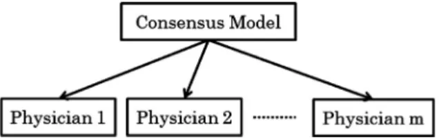
To address the above issues, we propose a new multi-expert learning framework that starts from data labeled by multiple ex-perts and builds: (1) aconsensus modelrepresenting the classifica-tion model the experts collectively converge to, and (2)individual expert modelsrepresenting the class label decisions exhibited by individual experts.Fig. 1shows the relations between these two components: the experts’ specific models and the consensus model. We would like to emphasize again that our framework builds the consensus model without access to any consensus/ meta labels.

To represent relations among the consensus and expert models, our framework considers different sources of disagreement that may arise when multiple experts label a case and explicitly represents them in the combined multi-expert model. In particular our framework assumes the following sources for expert disagreements:

Differences in the risks annotators associate with each class label assignment: diagnosing a patient as not having a disease when the patient has disease, carries a cost due to, for example, a missed opportunity to treat the patient, or longer patient dis-comfort and suffering. A similar, but different cost is caused by incorrectly diagnosing a patient. The differences in the expert-specific utilities (or costs) may easily explain differences in their label assessments. Hence our goal is to develop a learn-ing framework that seeks a model consensus, and that, at the same time, permits experts who have different utility biases. Differences in the knowledge (or model) experts use to label

exam-ples: while diagnoses provided by different experts may be often consistent, the knowledge they have and features they consider when making the disease decision may differ, poten-tially leading to differences in labeling. It is not rare when two expert physicians disagree on a complex patient case due to differences firmly embedded in their knowledge and under-standing of the disease. These differences are best characterized as differences in their knowledge or model they used to diag-nose the patient.

Differences in time annotators spend when labeling each case: dif-ferent experts may spend difdif-ferent amount of time and care to analyze the same case and its subtleties. This may lead to label-ing inconsistency even within the expert’s own model. We experiment with and test our multi-expert framework on the Heparin Induced Thrombocytopenia (HIT)[23]problem where our goal is to build a predictive model that can, as accurately as possible, assess the risk of the patient developing the HIT condition and predict HIT alerts. We have obtained the HIT alert annotations from three different experts in clinical pharmacy. In addition we have also acquired a meta-annotation from the fourth (senior) ex-pert who in addition to patient cases have seen the annotations and assessments given by other three experts. We show that our framework outperforms other machine learning frameworks (1) when it predicts a consensus label for future (test) patients and (2) when it predicts individual future expert labels.

2. Background

The problem of learning accurate classification models from clinical data that are labeled by human experts with respect to some condition of interest is important for many applications such as diagnosis, adverse event detection, monitoring and alerting, and the design of recommender systems.

Standard classification learning framework assumes the train-ing data setD¼ fðxi;yiÞg

n

i¼1consists ofndata examples, wherexi

is a d-dimensional feature vector andyiis a corresponding binary

class label. The objective is to learn a classification function: f:x?ythat generalizes well to future data.

The key assumption for learning the classification functionfin the standard framework is that examples in the training dataD are independent and generated by the same (identical) process, hence there are no differences in the label assignment process. However, in practice, especially in medicine, the labels are pro-vided by different humans. Consequently, they may vary and are subject to various sources of subjective bias and variations. We de-velop and study a newmulti-expert classification learning framework for which labels are provided by multiple experts, and that ac-counts for differences in subjective assessments of these experts when learning the classification function.

Briefly, we havemdifferent experts who assign labels to exam-ples. LetDk

¼ xk i;yki

nk

i¼1denotes training data specific for the ex-pertk, such thatxk

i is a d-dimensional input example and yki is

binary label assigned by expertk. Given the data from multiple ex-perts, our main goal is to learn the classification mapping:f:x?y that would generalize well to future examples and would repre-sent a good consensus model for all these experts. In addition, we can learn the expert specific classification functionsgk:x?yk

for allk= 1,. . .,mthat predicts as accurately as possible the label assignment for that expert. The learning offis a difficult problem because (1) the experts’ knowledge and reliability could vary and (2) each expert can have different preferences (or utilities) for dif-ferent labels, leading to difdif-ferent biases towards negative or posi-tive class. Therefore, even if two experts have the same relaposi-tive understanding of a patient case their assigned labels may be differ-ent. Under these conditions, we aim to combine the subjective la-bels from different experts to learn a good consensus model.

2.1. Related work

Methodologically our multi-expert framework builds upon models and results in two research areas:multi-task learningand learning-from-crowds, and combines them to achieve the above goals.

The multi-task learning framework [9,27] is applied when we want to learn models for multiple related (correlated) tasks. This framework is used when one wants to learn more efficiently the model by borrowing the data, or model components from a related task. More specifically, we can view each expert and his/her labels as defining a separate classification task. The multi-task learning framework then ties these separate but related tasks together, which lets us use examples labeled by all experts to learn better individual expert models. Our approach is motivated and builds upon the multi-task framework proposed by Evgeniou and Pontil

[9] that ties individual task models using a shared task model. However, we go beyond this framework by considering and mod-eling the reliability and biases of the different experts.

The learning-from-crowds framework[17,18]is used to infer con-sensus on class labels from labels provided jointly by multiple annotators (experts). The existing methods developed for the prob-lem range from the simple majority approach to more complex consensus models representing the reliability of different experts.

In general the methods developed try to either (1) derive a consen-sus of multiple experts on the label of individual examples or (2) build a model that defines the consensus for multiple experts and can be applied to future examples. We will review these in the following.

The simplest and most commonly used approach for defining the label consensus on individual examples is the majority voting. Briefly, the consensus on the labels for an example is the label as-signed by the majority of reviewers. The main limitation of the majority voting approach is that it assumes all experts are equally reliable. The second limitation is that although the approach defines the consensus on labels for existing examples, it does not directly de-fine a consensus model that can be used to predict consensus labels for future examples; although one may use the labels obtained from majority voting to train a model in a separate step.

Improvements and refinements of learning a consensus label or model take into account and explicitly model some of the sources of annotator disagreements. Sheng et al.[17]and Snow et al.[18]

showed the benefits of obtaining labels from multiple non-experts and unreliable annotators. Dawid and Skene[8]proposed a learn-ing framework in which biases and skills of annotators were mod-eled using a confusion matrix. This work was later generalized and extended in[25,24,26]by modeling difficulty of examples. Finally, Raykar et al. [14]used an expectation–maximization (EM) algo-rithm to iteratively learn the reliability of annotators. The initial reliability estimates were obtained using the majority vote.

The current state-of-the-art learning methods with multiple human annotators are the works of Raykar et al.[14], Welinder et al.[24], and Yan et al.[26]. Among these, only Raykar et al.

[14]uses a framework similar to the one we use in this paper; that is, it assumes (1) not all examples are labeled by all experts and (2) the objective is to construct a good classification model. However, the model differs from our approach in how it models the skills and biases of the human annotators. Also the authors in[14]show that their approach improves over simple baselines only when the number of annotators is large (more than 40). This is practical when the labeling task is easy so crowd-sourcing services like Amazon Mechanical Turk can be utilized. However, it is not practi-cal in domains in which the annotation is time consuming. In real world or scientific domains that involve uncertainty, including medicine, it is infeasible to assume the same patient case is labeled in parallel by many different experts. Indeed the most common cases is when every patient instance is labeled by just one expert. The remaining state-of-the-art learning from crowds methods, i.e. the works of Welinder et al.[24]and Yan et al.[26], are opti-mized for different settings than ours. Welinder et al.[24]assumes that there is no feature vector available for the cases; it only learns expert specific modelsgks, and it does not attempt to learn a

con-sensus modelf. On the other hand, Yan et al.[26]assumes that each example is labeled by all experts in parallel. As noted earlier, this is unrealistic, and most of the time each example is labeled only by one expert. The approach we propose in this paper over-comes these limitations and is flexible in that it can learn the mod-els when there is one or more labmod-els per example. In addition, our approach differs from the work of Yan et al.[26]in how we param-eterize and optimize our model.

3. Methodology

We aim to combine data labeled by multiple experts and build (1) a unified consensus classification modelffor these experts and (2) expert-specific modelsgk, for allk= 1,. . .,mthat can be applied

to future data.Fig. 2illustrates the idea of our framework with lin-ear classification models. Briefly, let us assume a linlin-ear consensus model f with parameters (weights) u and b from which linear

expert-specific modelsgks with parameters wkandbkare

gener-ated. Given the consensus model, the consensus label on example xis positive ifuT

x+bP0, otherwise it is negative. Similarly, the expert modelgkfor expertkassigns a positive label to examplex

if wT

kxþbkP0, otherwise the label is negative. To simplify the

notation in the rest of the paper, we include the bias termbfor the consensus model in the weights vector u, the biases bk in

wks, and extend the input vectorxwith constant 1.

The consensus and expert models in our framework and their labels are linked together using two reliability parameters:

1.

ak

: the self-consistency parameter that characterizes how reli-able the labeling of expertkis; it is the amount of consistency of expertkwithin his/her own modelwk.

2. bk: the consensus-consistency parameter that models how

con-sistent the model of expertkis with respect to the underlying consensus modelu. This parameter models the differences in the knowledge or expertise of the experts.

We assume, all deviations of the expert specific models from the consensus model are adequately modeled by these expert-specific reliability parameters. In the following we present the details of the overall model and how reliability parameters are incorporated into the objective function.

3.1. Multiple Experts Support Vector Machines (ME-SVM)

Our objective is to learn the parameters u of the consensus model and parameterswkfor all expert-specific models from the

data. We combine this objective with the objective of learning the expert specific reliability parameters

ak

andbk. We have

ex-pressed the learning problem in terms of the objective function based on the max-margin classification framework[16,19]which is used, for example, by support vector machines (SVMs). However, due to its complexity we motivate and explain its components using an auxiliary probabilistic graphical model that we later mod-ify to obtain the final max-margin objective function.

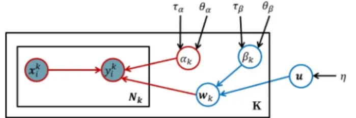
Fig. 3shows the probabilistic graphical model representation

[5,13] that refines the high level description presented inFig. 2. Briefly, the consensus modeluis defined by a Gaussian distribu-tion with zero mean and precision parameter

g

as:

pðuj0d;

g

Þ ¼ N ð0d;

g

1IdÞ ð1Þ

Fig. 2.The experts’ specific linear modelswkare generated from the consensus

linear modelu. The circles show instances that are mislabeled with respect to individual expert’s models and are used to define the model self consistency.

whereIdis the identity matrix of sized, and0dis a vector of sized

with all elements equal to 0. The expert-specific models are gener-ated from a consensus modelu. Every expert k has his/her own spe-cific modelwkthat is a noise corrupted version of the consensus

modelu; that is, we assume that expertk,wk, is generated from a

Gaussian distribution with meanuand an expert-specific precision bk:

pðwkju;bkÞ ¼ N u;b1k Id

The precision parameterbkfor the expertkdetermines how much

wkdiffers from the consensus model. Briefly, for a small bk, the

modelwktends to be very different from the consensus modelu,

while for a largebkthe models will be very similar. Hence,bk

rep-resents the consistency of the reviewer specific model wk with

the consensus modelu, or, in short, consensus-consistency. The parameters of the expert modelwkrelate examples (and

their features)xto labels. We assume this relation is captured by the regression model:

p yk ijx k i;wk;

a

k ¼ N wT kx k i;

a

1 k

where

ak

is the precision (inverse variance) and models the noise that may corrupt expert’s label. Hence

ak

defines the self-consis-tency of expertk. Please also note that althoughyk

i is binary,

simi-larly to [9,27], we model the label prediction and related noise using the Gaussian distribution. This is equivalent to using the squared error loss as the classification loss.

We treat the self-consistency and consensus-consistency parameters

ak

andbkas random variables, and model their priors

using Gamma distributions. More specifically, we define:

pðbkjhb;

s

bÞ ¼ Gðhb;

s

bÞ pð

a

kjha;

s

aÞ ¼ Gðha;

s

aÞ

ð2Þ where hyperparametershbkand

s

bkrepresent the shape and the in-verse scale parameter of the Gamma distribution representingbk.

Similarly,hakand

s

akare the shape and the inverse scale parameter of the distribution representing

ak

.

Using the above probabilistic model we seek to learn the parameters of the consensusuand expert-specific modelsWfrom data. Similarly to Raykar et al.[14]we optimize the parameters of the model by maximizing the posterior probabilityp(u,W,

a

,bjX,y, n), wherenis the collection of hyperparameters

g

;hbk;

s

bk;hak;

s

ak. The posterior probability can be rewritten as follows:

pðu;W;a;bjX;y;nÞ /pðuj0d;gÞ

Ym k¼1 pðbkjhb;sbÞpðakjha;saÞpðwkju;bkÞ Ynk i¼1 p yk ijx k i;ak;wk ! ð3Þ where X¼ x1 1; . . . ;x1n1; . . . ;x m 1; . . . ;xmnm h i

is the matrix of examples labeled by all the experts, and y¼ y1

1; . . . ;y1n1; . . . ;y 1

m; . . . ;ymnm

h i

are their corresponding labels. Similarly,Xk_andyk_{are the}

exam-ples and their labels from expertk. Direct optimization (maximi-zation) of the above function is difficult due to the complexities caused by the multiplication of many terms. A common optimiza-tion trick to simplify the objective funcoptimiza-tion is to replace the ori-ginal complex objective function with the logarithm of that function. This conversion reduces the multiplication to summa-tion [5]. Logarithm function is a monotonic function and leads to the same optimization solution as the original problem. Nega-tive logarithm is usually used to cancel many negaNega-tive signs pro-duced by the logarithm of exponential distributions. This changes the maximization to minimization. We follow the same practice and take the negative logarithm of the above expression to obtain the following problem (see Appendix A for the details of the derivation): min u;w;a;b

g

2kuk 2 þ1 2 Xm k¼1

a

k Xnk i¼1 yk iw T kx k i 2 þ1 2 Xm k¼1 bkkwkuk2 þX m k¼1 ðlnðbkÞ nklnð

a

kÞÞ þ Xm k¼1 ððhbk1ÞlnðbkÞ þ

s

bkbkÞ þX m k¼1 ððhak1Þlnð

a

kÞ þ

s

ak

a

kÞ ð4Þ

Although we can solve the objective function in Eq.(4)directly, we replace the squared error function in Eq.(4)with the hinge loss1_{for two reasons: (1) the hinge loss function is a tighter}

surro-gate for the zero-one (error) loss used for classification than the squared error loss[15]and (2) the hinge loss function leads to the sparse kernel solution[5]. Sparse solution means that the decision boundary depends on a smaller number of training examples. Sparse solutions are more desirable specially when the models are extended to non-linear case where the similarity of the unseen examples needs to be evaluated with respect to the training examples on which the decision boundary is dependent. By replacing the squared errors with the hinge loss we obtain the following objective function: min u;w;a;b

g

2kuk 2 þ1 2 Xm k¼1

ak

X nk i¼1 max 0;1yk iwTkxkiÞ þ1 2 Xm k¼1 bkkwkuk2þ Xm k¼1 ðlnðbkÞ nklnð

ak

ÞÞ þX m k¼1 ððhbk1ÞlnðbkÞ þ

s

bkbkÞ þ Xm k¼1 ððhak1Þlnð

ak

Þ þ

s

ak

ak

Þ ð5Þ We minimize the above objective function with respect to the consensus modelu, the expert specific modelwk, and expert

spe-cific reliability parameters

ak

andbk.

3.2. Optimization

We need to optimize the objective function in Eq.(5)with re-gard to parameters of the consensus modelu, the expert-specific modelswk, and expert-specific parameters

ak

andbk.

Similarly to the SVM, the hinge loss term: max 0;1yk iwTkxki

in Eq.(5)can be replaced by a constrained optimization problem with a new parameter

k

i. Briefly, from the optimization theory,

the following two equations are equivalent[6]:

Fig. 3.Graphical representation of the auxiliary probabilistic model that is related to our objective function. The circles in the graph represent random variables. Shaded circles are observed variables, regular (unshaded) circles denote hidden (or unobserved) random variables. The rectangles denote plates that represent structure replications, that is, there are k different expert modelswk, and each is

used to generate labels forNkexamples. Parameters not enclosed in circles (e.g.g)

denote the hyperparameters of the model.

1

Hinge loss is a loss function originally designed for training large margin classifiers such as support vector machines. The minimization of this loss leads to a classification decision boundary that has the maximum distance to the nearest training example. Such a decision boundary has interesting properties, including good generalization ability[15,21].

min wk max 0;1yk iw T kxki and min k i;wk

k i s:t: yk iw T kx k i >1

k i

Now replacing the hinge loss terms in Eq.(5), we obtain the equivalent optimization problem:

min u;w;;a;b

g

2kuk 2 þ1 2 Xm k¼1

a

k Xnk i¼1

k i þ1 2 Xm k¼1 bkkwkuk2 þX m k¼1 ðlnðbkÞ nklnð

a

kÞÞ þX m k¼1 ððhbk1ÞlnðbkÞ þ

s

bkbkÞ þX m k¼1 ððhak1Þlnð

a

kÞ þ

s

ak

a

kÞ s:t: yk iw T kx k i P1

k i; k¼1 m; i¼1 nk

k i P0; k¼1 m; i¼1 nk ð6Þ

where

denote the new set of

k

i parameters.

We optimize the above objective function using the alternating optimization approach [4]. Alternating optimization splits the objective function into two (or more) easier subproblems, each de-pends only on a subset of (hidden/learning) variables. After initial-izing the variables, it iterates over optiminitial-izing each set by fixing the other set until there is no change of values of all the variables. For our problem, diving the learning variables into two subsets, {

a

,b} and {u,w} makes each subproblem easier, as we describe below. After initializing the first set of variables, i.e.

ak

= 1 andbk= 1, we

iterate by performing the following two steps in our alternating optimization apparoach:

Learninguandwk: In order to learn the consensus modeluand

expert specific modelwk, we consider the reliability parameters

ak

andbkas constants. This will lead to an SVM form

optimiza-tion to obtainuandwk. Notice that

ki is also learned as part of

SVM optimization.

Learning

ak

andbk: By fixingu,wkfor all experts, and

, we can

minimize the objective function in Eq. (6) by computing the derivative with respect to

a

andb. This results in the following closed form solutions for

ak

andbk:

a

k¼ 2ðnkþhak1Þ P yk i¼1

k i þ2

s

ak ð7Þ bk¼ 2hbk kwkuk2þ2

s

bk ð8Þ Notice that

k

i is the amount of violation of label constraint for

examplexk

i (i.e. theith example labeled by expertk) thus

P

i¼1

ki

is the summation of all labeling violations for model of expertk. This implies that

ak

is inversely proportional to the amount of mis-classification of examples by expertkaccording to its specific model wk. As a result,

ak

represents the consistency of the labels provided

by expertkwith his/her own model.bkis inversely related to the

difference of the model of expert k (i.e. wk) with the consensus

modelu. Thus it is the consistency of the model learned for expert kfrom the consensus modelu.

4. Experimental evaluation

We test the performance of our methods on clinical data obtained from EHRs for post-surgical cardiac patients and the problem of monitoring and detection of the Heparin Induced Thrombocytope-nia (HIT)[23,22]. HIT is an adverse immune reaction that may devel-op if the patient is treated for a longer time with heparin, the most common anticoagulation treatment. If the condition is not detected and treated promptly it may lead to further complications, such as thrombosis, and even to patient’s death. An important clinical prob-lem is the monitoring and detection of patients who are at risk of developing the condition. Alerting when this condition becomes likely prevents the aggravation of the condition and appropriate countermeasures (discontinuation of the heparin treatment or switch to an alternative anticoagulation treatment) may be taken. In this work, we investigate the possibility of building a detector from patient data and human expert assessment of patient cases with respect to HIT and the need to raise the HIT alert. This corre-sponds to the problem of learning a classification model from data where expert’s alert or no-alert assessments define class labels. 4.1. Data

The data used in the experiments were extracted from over 4486 electronic health records (EHRs) in Post-surgical Cardiac Pa-tient (PCP) database[11,20,12]. The initial data consisted of over 51,000 unlabeled patient-state instances obtained by segmenting each EHR record in time with 24-h period. Out of these we have se-lected 377 patient instances using a stratified sampling approach that were labeled by clinical pharmacists who attend and manage patients with HIT. Since the chance of observing HIT is relatively low, the stratified sampling was used to increase the chance of observing patients with positive labels. Briefly, a subset of strata covered expert-defined patterns in the EHR associated with the HIT or its management, such as, the order of the HPF4 lab test used to confirm the condition[22]. We asked three clinical pharmacists to provide us with labels showing if the patient is at the risk of HIT and if they would agree to raise an alert on HIT if the patient was encountered prospectively. The assessments were conducted using a web-based graphical interface (called PATRIA) we have devel-oped to review EHRs of patients in the PCP database and their in-stances. All three pharmacists worked independently and labeled all 377 instances. After the first round of expert labeling (with three experts) we asked a (senior) expert on HIT condition to label the data, but this time, the expert in addition to information in the EHR also had access to the labels of the other three experts. This process led to 88 positive and 289 negative labels. We used the judgement and labels provided by this expert as consensus labels. We note that alternative ways of defining consensus labels in the study would be possible. For example, one could ask the senior expert to label the cases independent of labels of other reviewers and consider expert’s labels as surrogates for the consensus labels. Similarly one can ask all three experts to meet and resolve the cases they disagree on. However, these alternative designs come with the different limitations. First, not seeing the labels of other reviewers the senior expert would make a judgment on the labels on her own and hence it would be hard to speak about consensus labels. Second, the meeting of the experts and the resolution of the differences on every case in the study in person would be hard to arrange and time consuming to undertake. Hence, we see the op-tion of using senior expert’s opinion to break the ties as a reason-able alternative that (1) takes into account labels from all experts and (2) resolves them without arranging a special meeting of all experts involved.

In addition, we would like to emphasize that the labels provided by the (senior) expert were only used to evaluate the quality of the different consensus models. That is, we did not use the labels pro-vided by that expert when training the different consensus models, and only applied them in the evaluation phase.

4.2. Temporal feature extraction

The EHR consists of complex multivariate time series data that reflect sequences of lab values, medication administrations, proce-dures performed, etc. In order to use these for building HIT predic-tion models, a small set of temporal features representing well the patient state with respect to HIT for any timetis needed. However, finding a good set of temporal features is an extremely challenging task [10,2,7,3,1]. Briefly, the clinical time series, are sampled at irregular times, have missing values, and their length may vary depending on the time elapsed since the patient was admitted to the hospital. All these make the problem of summarizing the infor-mation in the time series hard. In this work, we address the above issues by representing the patient state at any (segmentation) time t using a subset of pre-defined temporal feature mappings pro-posed by Hauskrecht et al.[11,20,12]that let us convert patient’s information known at timetto a fixed length feature vector. The feature mappings define temporal features such as last observed platelet count value, most recent platelet count trend, or, the length of time the patient is on medication.Fig. 4illustrates a sub-set of 10 feature mappings (out of 14) that we applied to summa-rize time series for numeric lab tests. We used feature mappings for five clinical variables useful for the detection of HIT: Platelet counts, Hemoglobin levels, White Blood Cell Counts, Heparin administration record, Major heart procedure. The full list of fea-tures generated for these variables is listed inAppendix B. Briefly, temporal features for numeric lab tests: Platelet counts, Hemoglo-bin levels and White Blood Cell Counts used feature mappings illustrated inFig. 4plus additional features representing the pres-ence of last two values, and pending test. The heparin features summarize if the patient is currently on the heparin or not, and the timing of the administration, such as the time elapsed since the medication was started, and the time since last change in its administration. The heart procedure features summarize whether the procedure was performed or not and the time elapsed since the last and first procedure. The feature mappings when applied to EHR data let us map each patient instance to a vector of 50 fea-tures. These features were then used to learn the models in all sub-sequent experiments. The alert labels assigned to patient instances by experts were used as class labels.

4.3. Experimental set-up

To demonstrate the benefits of our multi-expert learning frame-work we used patient instances labeled by four experts as outlined above. The labeled data were randomly split into the training and

test sets, such that 2/3 of examples were used for training exam-ples and 1/3 for testing. We trained all models in the experimental section on the training set and evaluated on the test set. We used the Area Under the ROC Curve (AUC) on the test set as the main statistic for all comparisons. We repeated train/test split 100 times and report the average and 95% confidence interval. We compare the following algorithms:

SVM-baseline: This is a model obtained by training a linear SVM classifier that considers examples and their labels and ignores any expert information. We use the model as a baseline. Majority: This model selects the label in the training data using

the majority vote and learns a linear SVM classifier on examples with the majority label. This model is useful only when multiple experts label the same patient instance. Notice that SVM and Majority performs exactly the same if each example is labeled by one and only one expert.

Raykar: This is the algorithm and model developed by Raykar et al.[14]. We used the same setting as discussed in[14]. ME-SVM: This is the new method we propose in this paper. We

set the parameters

g

=

s

a=

s

b= 1,ha=hb= 1.

SE-SVM: Senior-Expert-SVM (SE-SVM) is the SVM model trained using the consensus labels provided by our senior pharmacist. Note that this method does not derive a consensus model from labels given by multiple experts; instead, it ‘cheats’ and learns consensus model directly from consensus labels. This model and its results are used for comparison purposes only and serve as the reference point.

We investigate two aspects of the proposed ME-SVM method: 1. The performance of the consensus model on the test data when

it is evaluated on the labels provided by the senior expert on HIT.

2. The performance of the expert-specific model wkfor expertk

when it is evaluated on the examples labeled by that expert. 4.4. Results and discussion

4.4.1. Learning consensus model

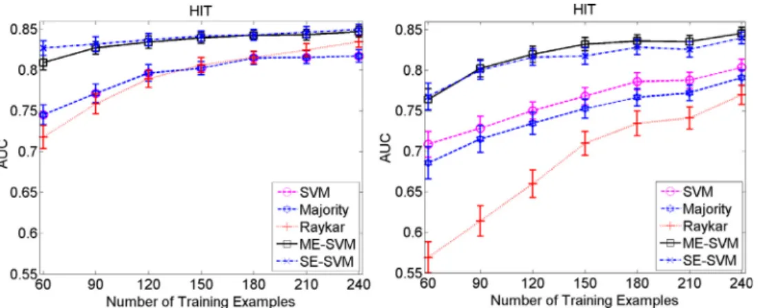
The cost of labeling examples in medical domain is typically very high, so in practice we may have a very limited number of training data. Therefore, it is important to have a model that can efficiently learn from a small number of training examples. We investigate how different methods perform when the size of train-ing data varies. For this experiment we randomly sample examples from the training set to feed the models and evaluate them on the test set. We simulated and tested two different ways of labeling the examples used for learning the model: (1) every example was given to just one expert, and every expert labeled the same number of examples and (2) every example was given to all ex-perts, that is, every example was labeled three times. The results

are shown inFig. 5. Thex-axis shows the total number of cases la-beled by the experts. The left and right plots respectively show the results when labeling options 1 and 2 are used.

First notice that our method that explicitly models experts’ dif-ferences and their reliabilities consistently outperforms other con-sensus methods in both strategies, especially when the number of training examples is small. This is particularly important when la-bels are not recorded in the EHRs and must be obtained via a sep-arate post-processing step, which can turn out to be rather time-consuming and requires additional expert effort. In contrast to our method the majority voting does not model the reliability of different experts and blindly considers the consensus label as the majority vote of labels provided by different experts. The SVM method is a simple average of reviewer specific models and does not consider the reliability of different experts in the combination. The Raykar method, although modeling the reliabilities of different experts, assumes that the experts have access to the label gener-ated by the consensus model and report a perturbed version of the consensus label. This is not realistic because it is not clear why the expert perturb the labels if they have access to consensus model. In contrary, our method assumes that different experts aim to use a model similar to consensus model to label the cases how-ever their model differs from the label of the consensus model be-cause of their differences in the domain knowledge, expertise and utility functions. Thus, our method uses a more intuitive way and realistic approach to model the label generating process.

Second, by comparing the two strategies for labeling patient in-stances we see that option 1, where each reviewer labels different patient instances, is better (in terms of the total labeling effort) than option 2 where all reviewers label the same instances. This shows that the diversity in patient examples seen by the frame-work helps and our consensus model is improving faster, which is what we intuitively expect.

Finally, note that our method performs very similarly to the SE-SVM – the model that ‘cheats’ and is trained directly on the con-sensus labels given by the senior pharmacist. This verifies that our framework is effective in finding a good consensus model with-out having access to the consensus labels.

4.4.2. Modeling individual experts

One important and unique feature of our framework when com-pared to other multi-expert learning frameworks is that it models explicitly the individual experts’ modelswk, not just the consensus

modelu. In this section, we study the benefit of the framework for learning the expert specific models by analyzing how the model for any of the experts can benefit from labels provided by other ex-perts. In other words we investigate the question:Can we learn

an expert model better by borrowing the knowledge and labels from other experts? We compared the expert specific models learned by our framework with the following baselines:

SVM: We trained a separate SVM model for each expert using patient instances labeled only by that expert. We use this model as a baseline.

Majority⁄_{: This is the Majority model described in the previous} section. However, since Majority model does not give expert specific models, we use the consensus model learned by the Majority method in order to predict the labels of each expert. Raykar⁄_{: This is the model developed by Raykar et al.[14], as}

described in the previous section. Similarly to Majority, Raykar’s model does not learn expert specific models. Hence, we use the consensus model it learns to predict labels of individual experts. ME-SVM: This is the new method we propose in this paper, that

generates expert specific models as part of its framework. Similarly to Section 4.4.1, we assume two different ways of labeling the examples: (1) every example was given to just one ex-pert, and every expert labeled the same number of examples and (2) every example was given to all experts, that is every example was labeled three times.

We are interested in learning individual prediction models for three different experts. If we have a budget to label some number of patient instances, say, 240, and give 80 instances to each expert, then we have can an individual expert model from: (1) all 240 examples by borrowing from the instances labeled by the other ex-perts or (2) only its own 80 examples. The hypothesis is that learn-ing from data and labels given by all three experts collectively is better than learning each of them individually. The hypothesis is also closely related to the goal of multi-task learning, where the idea is to use knowledge, models or data available for one task to help learning of models for related domains.

The results for this experiment are summarized inFig. 6, where x-axis is the number of training examples fed to the models andy -axis shows how well the models can predict individual experts’ la-bels in terms of the AUC score. The first (upper) line of sub-figures shows results when each expert labels a different set of patient in-stances, whereas the second (lower) line of sub-figures shows re-sults when instances are always labeled by all three experts. The results show that our ME-SVM method outperforms the SVM trained on experts’ own labels only. This confirms that learning from three experts collectively helps to learn expert-specific mod-els better than learning from each expert individually and that our framework enables such learning. In addition, the results of Major-ity⁄_{and Raykar}⁄_{methods show that using their consensus models}

Fig. 5.Effect of the number of training examples on the quality of the model when: (Left) every example is labeled by just one expert and (Right) every example is labeled by all three experts.

to predict expert specific labels is not as effective and that their performance is worse than our framework that relies on expert specific models.

4.4.3. Self-consistency and consensus-consistency

As we described in Section3, we model self-consistency and consensus-consistency with parameters

ak

and bk.

ak

measures

60 90 120 150 180 210 240 0.55 0.6 0.65 0.7 0.75 0.8 0.85 HIT, reviewer 1

Number of Training Examples

AUC SVM Majority* Raykar* ME−SVM 60 90 120 150 180 210 240 0.55 0.6 0.65 0.7 0.75 0.8 0.85 HIT, reviewer 2

Number of Training Examples

AUC SVM Majority* Raykar* ME−SVM 60 90 120 150 180 210 240 0.55 0.6 0.65 0.7 0.75 0.8 0.85 HIT, reviewer 3

Number of Training Examples

AUC SVM Majority* Raykar* ME−SVM 60 90 120 150 180 210 240 0.55 0.6 0.65 0.7 0.75 0.8 0.85 HIT, reviewer 1

Number of Training Examples

AUC SVM Majority* Raykar* ME−SVM 60 90 120 150 180 210 240 0.55 0.6 0.65 0.7 0.75 0.8 0.85 HIT, reviewer 2

Number of Training Examples

AUC SVM Majority* Raykar* ME−SVM 60 90 120 150 180 210 240 0.55 0.6 0.65 0.7 0.75 0.8 0.85 HIT, reviewer 3

Number of Training Examples

AUC

SVM Majority* Raykar* ME−SVM

Fig. 6.Learning of expert-specific models. The figure shows the results for three expert specific models generated by the ME-SVM and the standard SVM methods, and compares them to models generated by the Majority⁄

and Raykar⁄

methods. First line: different examples are given to different experts and Second line: the same examples are given to all experts.

30 60 90 120 150 180 210 240 0.83 0.84 0.85 0.86 0.87 0.88 0.89

Number of Training Examples

Agreement with Consensus

0 30 60 90 120 150 180 210 240 0.3 0.31 0.32 0.33 0.34 0.35 0.36 0.37

Number of Training Examples

Normalized Self−Consistency 0 30 60 90 120 150 180 210 240 0.3 0.32 0.34 0.36 0.38 0.4 0.42

Number of Training Examples

Normalized Reviewer 1 Reviewer 2 Reviewer 3 Reviewer 1 Reviewer 2 Reviewer 3 Reviewer 1 Reviewer 2 Reviewer 3 0 30 60 90 120 150 180 210 240 0.6 0.65 0.7 0.75

Number of Training Examples

Consensus + Self Consistency

Reviewer 1 Reviewer 2 Reviewer 3

Consensus−Consistency

Labels

Fig. 7.(left-top) Agreement of experts with labels given by the senior expert; (right-top) learned self-consistency parameters for Experts 1–3; (left-bottom) learned consensus-consistency parameters for Experts 1–3; (right-bottom) cumulative self and consensus consistencies for Expert 1–3.

how consistent the labeling of expertkis with his/her own model and bkmeasures how consistent the model of expertkis with respect to

the consensus model. The optimization problem we proposed in Eq.

(6)aims to learn not just the parametersuandwkof the consensus

and experts’ models, but also the parameters

ak

andbk, and this

with-out having access to the labels from the senior expert.

In this section, we attempt to study and interpret the values of the reliability parameters as they are learned by our framework and compare them to empirical agreements in between the senior (defining the consensus) and other experts.Fig. 7a shows the agree-ments of labels provided by the three experts with labels given by the senior expert, which we assumed gives the consensus labels. From this figure we see that Expert 2 agrees with the consensus la-bels the most, followed by Expert 3 and then Expert 1. The agree-ment is measured in terms of the absolute agreeagree-ment, and reflects the proportion of instances for which the two labels agree.

Fig. 7b and c show the values of the reliability parameters

a

and b, respectively. Thex-axis in these figures shows how many train-ing patient instances per reviewer are fed to the model. Normal-ized self-consistency in Fig. 7b is the normalized value of

ak

in Eq.(6). Normalized consensus-consistency inFig. 7c is the normal-ized inverse value of Euclidean distance between an expert specific model and consensus model: 1/kwkuk, which is proportional to

bkin Eq.(6). InFig. 7d we add the two consistency measures in an

attempt to measure the overall consistency in between the senior expert (consensus) and other experts.

As we can see, at the beginning when there is no training data all experts are assumed to be the same (much like the majority voting approach). However, as the learning progresses with more training examples available, the consistency measures are updated and their values define the contribution of each expert to the learning of con-sensus model: the higher the value the larger the contribution.

Fig. 7b shows that expert 3 is the best in terms of self-consistency gi-ven the linear model, followed by expert 2 and then expert 1. This means expert 3 is very consistent with his model, that is, he likely gives the same labels to similar examples.Fig. 7c shows that expert 2 is the best in terms of consensus-consistency, followed by expert 3 and then expert 1. This means that although expert 2 is not very sistent with respect to his own linear model his model appears to con-verge closer to the consensus model. In other words, expert 2 is the closest to the expected consensus in terms of the expertise but devi-ates with some labels from his own linear model than expert 3 does.2

Fig. 7d shows the summation of the two consistency measures. By comparingFig. 7a and d we observe that the overall consistency mimics well the agreements in between the expert defining the con-sensus and other experts, especially when the number of patient in-stances labeled and used to train our model increases. This is encouraging, since the parameters defining the consistency mea-sures are learned by our framework only from the labels of the three experts and hence the framework never sees the consensus labels.

5. Conclusion

The construction of predictive classification models from clini-cal data often relies on labels reflecting subjective human assess-ment of the condition of interest. In such a case, differences among experts may arise leading to potential disagreements on the class label that is assigned to the same patient case. In this work, we have developed and investigated a new approach to com-bine class-label information obtained from multiple experts and

learn a common (consensus) classification model. We have shown empirically that our method outperforms other state-of-the-art methods when building such a model. In addition to learning a common classification model, our method also learns expert spe-cific models. This addition provides us with an opportunity to understand the human experts’ differences and their causes which can be helpful, for example, in education and training, or in resolv-ing disagreements in the patient assessment and patient care. Acknowledgements

This research work was supported by Grants R01LM010019 and R01GM088224 from the National Institutes of Health. Its content is solely the responsibility of the authors and does not necessarily represent the official views of the NIH.

Appendix A. Derivation of Eq. (4) from Eq. (3)

In this appendix, we give a more detailed derivation of Eq.(4)

from(3): pðu;W;

g

;

a

;bjX;y;nÞ /pðuj0d;

g

Þ Y m k¼1 pðbkjhb;

s

bÞpð

a

kjha;

s

aÞpðwkju;bkÞ Ynk i¼1 p yk ijxki;

a

k;wk ! ¼ Nuj0;b1k IdY m k¼1 Gðbkjhb;

s

bÞGð

a

kjha;

s

aÞN ðwkju;b1k IdÞ Y nk i¼1 N yk ijw>kx k i;

a

k ! ¼

g

_{ffiffiffiffiffiffiffi}k 2

p

p egku₂k2Y m k¼1 1

C

ðhbÞ

s

hb bb hb1 k e sbbk 1

C

ðhaÞ

s

ha a

a

h a1 k e saak bffiffiffiffiffiffiffik 2

p

p ebkkw_kuk2 2 Y nk i¼1

a

k ffiffiffiffiffiffiffi 2

p

p eak ykiw>kx k i k k2 2 !

Taking the negative logarithm ofpðu;W;

g

;

a

;bjX;y;nÞthat lets us to convert the maximization problem to minimization, we get:

lnpðu;W;

g

;

a

;bjX;y;nÞ ¼ lnð

g

Þ logðpffiffiffiffiffiffiffi2

p

Þ þ1 2

g

kuk 2 þX m k¼1 ðlnð

C

ðhbÞÞ hblnð

s

bÞ ðhb1ÞlnðbkÞ þ

s

bbkÞ þX m k¼1 ðlnð

C

ðhaÞÞ halnð

s

aÞ ðha1Þlnð

a

kÞ þ

s

a

a

kÞ þX m k¼1 lnðbkÞ þlnð ffiffiffiffiffiffiffi 2

p

p Þ þ1 2bkkwkuk2Þ þX m k¼1 Xnk i¼1 lnð

a

kÞ þlnð ffiffiffiffiffiffiffi 2

p

p Þ þ1 2

a

kky k iw > kx k ik 2

Rewriting the above equation we get: lnpðu;W;

g

;

a

;bjX;y;nÞ ¼ 1 2

g

kuk 2 þX m k¼1 ððhb1ÞlnðbkÞ þ

s

bbkÞ þX m k¼1 ððha1Þlnð

a

kÞ þ

s

a

a

kÞ þX m k¼1 lnðbkÞ þ 1 2bkkwkuk2 þX m k¼1 Xnk i¼1 lnð

a

kÞ þ 1 2

a

kky k i w > kx k ik 2 þA 2

We would like to note that the self-consistency and consensus-consistency parameters learned by our framework are learned together and hence it is possible one consistency measure may offset or compensate for the value of the other measure during the optimization. In that case the interpretation of the parameters as presented may not be as straightforward.

where Asums all constant terms that can be ignored during the optimization step, and that include terms involving hyperparame-ters

g

; ha;

s

a; hbthat are constants. By ignoringAand rearranging

the remaining terms we get Eq. 4.

Removing the constants terms (i.e. those related to

g

,ha,

s

a,hb

and

s

b, we will have:

1 2

g

kuk 2 þX m k¼1 ðhb1ÞlogðbkÞ þ

s

bbk ðha1Þlogð

a

kÞ þ

s

a

a

klogðbkÞ þ 1 2bkkwkuk2þ Xnk i¼1 logð

a

kÞ þ1 2

a

k y k i w>kx k i 2

Rearranging the terms in the above equation, we obtain Eq.(4). Appendix B. Features used for constructing the predictive models

SeeTable 1.

References

[1]Batal Iyad, Fradkin Dmitriy, Harrison James, Moerchen Fabian, Hauskrecht Milos. Mining recent temporal patterns for event detection in multivariate time series data. In: Proceedings of the international conference on Knowledge discovery and data mining. ACM; 2012. p. 280–8.

[2] Batal Iyad, Sacchi Lucia, Bellazzi Riccardo, Hauskrecht Milos. Multivariate time series classification with temporal abstractions. In: Proceedings of Florida Artificial intelligence research society conference; 2009.

[3]Batal Iyad, Valizadegan Hamed, Cooper Gregory F, Hauskrecht Milos. A pattern mining approach for classifying multivariate temporal data. In: IEEE international conference on bioinformatics and biomedicine (BIBM). IEEE; 2011. p. 358–65.

[4]Bezdek James C, Hathaway Richard J. Some notes on alternating optimization. In: Proceedings of the 2002 AFSS international conference on fuzzy systems. Calcutta: advances in soft computing, AFSS ’02. London, UK, UK: Springer-Verlag; 2002. p. 288–300.

[5]Bishop Christopher M. Pattern recognition and machine learning. Springer; 2006.

[6]Boyd Stephen, Vandenberghe Lieven. Convex optimization. New York, NY, USA: Cambridge University Press; 2004.

[7]Combi Carlo, Keravnou-Papailiou Elpida, Shahar Yuval. Temporal information systems in medicine. Springer Publishing Company, Incorporated; 2010. [8]Dawid AP, Skene AM. Maximum likelihood estimation of observer error-rates

using the em algorithm. Appl Stat 1979;28(1):20–8.

[9]Evgeniou Theodoros, Pontil Massimiliano. Regularized multi-task learning. In: Proceedings of the international conference on Knowledge discovery and data mining. New York, NY, USA: ACM; 2004. p. 109–17.

[10] Hauskrecht M, Fraser H. Modeling treatment of ischemic heart disease with partially observable markov decision processes. In: Proceedings of the AMIA annual symposium; 1998. p. 538–42.

[11] Hauskrecht M, Valko M, Batal I, Clermont G, Visweswaran S, Cooper GF. Conditional outlier detection for clinical alerting. In: Proceedings of the AMIA annual symposium; 2010. p. 286–890.

[12]Hauskrecht Milos, Batal Iyad, Valko Michal, Visweswaran Shyam, Cooper Gregory F, Clermont Gilles. Outlier detection for patient monitoring and alerting. J Biomed Inform 2013;46(1):47–55.

[13]Koller Daphne, Friedman Nir. Probabilistic graphical models: principles and techniques. MIT Press; 2009.

[14]Raykar VC, Yu S, Zhao LH, Valadez GH, Florin C, Bogoni L, et al. Learning from crowds. Journal of Machine Learning Research 2010;11:1297–322. [15]Scholkopf Bernhard, Smola Alexander J. Learning with kernels: support vector

machines, regularization, optimization, and beyond. Cambridge, MA, USA: MIT Press; 2001.

[16]Scholkopf Bernhard, Smola Alexander J. Learning with kernels: support vector machines, regularization, optimization, and beyond. Cambridge, MA, USA: MIT Press; 2002.

[17]Sheng Victor S, Provost Foster, Ipeirotis Panagiotis G. Get another label? Improving data quality and data mining using multiple, noisy labelers. In: Proceedings of the international conference on Knowledge discovery and data mining. ACM; 2008. p. 614–22.

[18]Snow Rion, O’Connor Brendan, Jurafsky Daniel, Ng Andrew Y. Cheap and fast— but is it good?: Evaluating non-expert annotations for natural language tasks. In: Conference on Empirical Methods on Natural Language Processing. Stroudsburg, PA, USA: Association for Computational Linguistics; 2008. p. 254–63.

[19]Valizadegan Hamed, Jin Rong. Generalized maximum margin clustering and unsupervised kernel learning. In: Schölkopf B, Platt J, Hoffman T, editors. Advances in neural information processing systems, vol. 19. Cambridge, MA: MIT Press; 2007. p. 1417–24.

[20] Valko Michal, Hauskrecht Milos. Feature importance analysis for patient management decisions. In: Proceedings of the 13th international congress on medical informatics; 2010. p. 861–5.

[21]Vapnik Vladimir N. The nature of statistical learning theory. New York, NY, USA: Springer-Verlag New York, Inc.; 1995.

Table 1

Features used for constructing the predictive models. The features were extracted from time series data in electronic health records using methods from Hauskrecht et al.[11,20,12].

Clinical variables Features

Platelet count (PLT) 1 Last PLT value measurement

2 Time elapsed since last PLT measurement 3 Pending PLT result

4 Known PLT value result indicator 5 Known trend PLT results

6 PLT difference for last two measurements 7 PLT slope for last two measurements 8 PLT % drop for last two measurements 9 Nadir HGB value

10 PLT difference for last and nadir values 11 Apex PLT value

12 PLT difference for last and apex values 13 PLT difference for last and baseline values 14 Overall PLT slope

Hemoglobin (HGB) 15 Last HGB value measurement

16 Time elapsed since last HGB measurement 17 Pending HGB result

18 Known HGB value result indicator 19 Known trend HGB results

20 HGB difference for last two measurements 21 HGB slope for last two measurements 22 HGB % drop for last two measurements 23 Nadir HGB value

24 HGB difference for last and nadir values 25 Apex HGB value

26 HGB difference for last and apex values 27 HGB difference for last and baseline values 28 Overall HGB slope

White Blood Cell count (WBC)

29 Last WBC value measurement

30 Time elapsed since last WBC measurement 31 Pending WBC result

32 Known WBC value result indicator 33 Known trend WBC results

34 WBC difference for last two measurements 35 WBC slope for last two measurements 36 WBC % drop for last two measurements 37 Nadir WBC value

38 WBC difference for last and nadir values 39 Apex WBC value

40 WBC difference for last and apex values 41 WBC difference for last and baseline values 42 Overall WBC slope

Heparin 43 Patient on Heparin

44 Time elapsed since last administration of Heparin

Table 1(continued)

Clinical variables Features

45 Time elapsed since first administration of Heparin

46 Time elapsed since last change in Heparin administration

Major heart procedure 47 Patient had a major heart procedure in past 24 h

48 Patient had a major heart procedure during the stay

49 Time elapsed since last major heart procedure

50 Time elapsed since first major heart procedure

[22]Warkentin TE. Heparin-induced thrombocytopenia: pathogenesis and management. Br J Haematol 2003:535–55.

[23]Warkentin TE, Sheppard JI, Horsewood P. Impact of the patient population on the risk for heparin-induced thrombocytopenia. Blood 2000:1703–8. [24] Welinder Peter, Branson Steve, Belongie Serge, Perona Pietro. The

multidimensional wisdom of crowds. In: Advances in neural information processing systems; 2010, 2424–2432.

[25] Whitehill Jacob, Ruvolo Paul, fan Wu Ting, Bergsma Jacob, Movellan Javier. Whose vote should count more: optimal integration of labels from labelers of

unknown expertise. In: Advances in neural information processing systems; 2009. p. 2035–43.

[26] Yan Yan, Fung Glenn, Dy Jennifer, Rosales Romer. Modeling annotator expertise: learning when everybody knows a bit of something. In: Proceedings of the international conference on Artificial Intelligence and Statistics; April 2010.

[27] Zhang Yu, Yeung Dit-Yan. A convex formulation for learning task relationships in multi-task learning. In: Proceedings of the international conference on the Uncertainty in Artificial Intelligence; 2010.