(will be inserted by the editor)
Multivariate Functional Outlier Detection
Mia Hubert · Peter Rousseeuw · Pieter Segaert
Received: date / Accepted: date
Abstract Functional data are occurring more and more often in practice, and var-ious statistical techniques have been developed to analyze them. In this paper we consider multivariate functional data, where for each curve and each time point a
p-dimensional vector of measurements is observed. For functional data the study of outlier detection has started only recently, and was mostly limited to univariate curves (p=1). In this paper we set up a taxonomy of functional outliers, and construct new numerical and graphical techniques for the detection of outliers in multivariate func-tional data, with univariate curves included as a special case. Our tools include sta-tistical depth functions and distance measures derived from them. The methods we study are affine invariant inp-dimensional space, and do not assume elliptical or any other symmetry.
Keywords Depth·Diagnostic plot·Functional data·Graphical display·Heatmap· Robustness
1 Introduction
Functional data are occurring more and more often in practice, and various statistical techniques have been developed to analyze this type of data. Standard references on functional data include Ramsay and Silverman (2002, 2006) and Ferraty and Vieu (2006). A functional data set typically consists ofncurves observed on a set of time pointst1, . . . ,tT. In this paper we consider multivariate functional data, where for
each curve and each time point ap-dimensional vector of measurements is observed. Several examples of multivariate functional data can be found in the literature. Popu-lar examples include the bivariate gait data set containing the simultaneous variation M. Hubert, P. Rousseeuw, P. Segaert
Department of Mathematics, KU Leuven, Celestijnenlaan 200B, BE-3001 Heverlee, Belgium Tel.: +32-16-322023
of the hip and knee angles of 39 children (Ramsay and Silverman, 2006). Berren-dero et al (2011) analyzed daily temperature data measured at 3, 9 and 12 cm below ground during 21 days. Another example is the multi-lead ECG data set analyzed by Pigoli and Sangalli (2012) for which p=8. Here, the data contain measurements of the human heart activity at 8 different places on the body.
Nowadays statisticians are well aware of the potential effects of outliers on data analysis, and there is an extensive literature on finding outliers and developing meth-ods that are robust to their influence; see e.g. Rousseeuw and Leroy (1987) and Maronna et al (2006). But for functional data the study of outlier detection has started only recently, and was mostly limited to univariate curves, i.e.p=1. Febrero-Bande et al (2008) identified two reasons why outliers can be present in functional data. First, gross errors can be caused by errors in measurements and recording or typ-ing mistakes, which should be identified and corrected if possible. Second, outliers can be correctly observed data curves that are suspicious or surprising in the sense that they do not follow the same pattern as that of the majority of the curves. Us-ing recorded NOx levels in Barcelona as a case study, Febrero-Bande et al (2008)
proposed the following outlier detection procedure for univariate functional data (i.e.
p=1), consisting of three main steps:
1. For each curve, calculate its functional depth (several versions exist); 2. delete observations with depth below a cutoffC;
3. go back to step 1 with the reduced sample, and repeat until no outliers are found. Step 3 was added in the hope of avoiding masking effects. The cutoff valueCwas obtained by a bootstrap procedure.
A different approach was taken by Hyndman and Shang (2010) who noted that the above method lacks sensitivity to curves whose pattern is different from the majority but whose values at each time point look inconspicuous. Hyndman and Shang (2010) considered the observed curves(Yi(t1), . . . ,Yi(tT))as multivariate observations inT
dimensions and applied a robust PCA method to them, keeping the first two princi-pal components. Next they computed the bagplot (Rousseeuw et al, 1999) of these bivariate points, or their highest density regions (Hyndman, 1996). However, it is not guaranteed that outliers can be detected by looking at the first two principal scores.
To visualize univariate functional data and investigate their spread as well as pos-sible outliers, Sun and Genton (2011) proposed the functional boxplot. This new boxplot is a generalization of the univariate boxplot using functional depth as a re-placement for the traditional univariate ranks. It shows, as a function of time, the deepest curve, the 50% central region (i.e. the envelope of the 50% deepest curves), and the fence. The latter is obtained by inflating the central region by 1.5 times its range. In this approach a curve is considered outlying if it ventures outside the fence in at least one time point.
The aims of this paper are twofold. We first set up a taxonomy of functional outliers in order to be able to classify different types of outlying behavior. Secondly, we construct new tools for the detection of outliers in multivariate functional data, with univariate curves included as a special case. These tools will aid in handling and interpreting outlying curves. For instance, curves with local gross errors should not necessarily be flagged as completely outlying, as this would lead to a substantial
loss of information. The proposed methods will be affine invariant in p-dimensional space, an important theoretical and practical benefit for multivariate curves. Also, we will not assume elliptical or any other symmetry.
In the next section we will discuss different types of functional outlyingness and set up a taxonomy. In Section 3 we discuss halfspace depth and extend its use to detect outliers in multivariate and functional data. Section 4 introduces the skew-adjusted projection depth and a new diagnostic plot. In Section 5 we apply our new techniques to real data sets, before presenting our conclusions.
2 Functional Outliers
2.1 Taxonomy of functional outliers
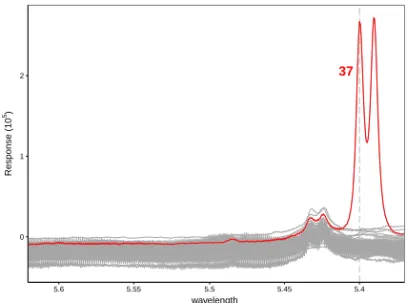
Functional observations can be deviating from the majority of the curves in various ways. First of all, we distinguishisolated outliersthat exhibit outlying behavior dur-ing a very short time interval. For univariate curves this type of outlydur-ingness reduces to one or more spikes or peaks. An illustration is given in Figure 1 which plots pro-ton nuclear magnetic resonance (NMR) spectra of 40 different wine samples (Larsen et al, 2006). The full data set contains measurements in the spectral region from 6.00 to 0.50, but for clarity we focus on the region between wavelengths 5.62 and 5.37 only, for whichT =397 measurements are available for each curve. The red curve 37 has large peaks around wavelength 5.4 and can be considered an isolated outlier.
37 0 1 2 5.6 5.55 5.5 5.45 5.4 wavelength Response (10 5)
Fig. 1 NMR spectra for 40 wine samples with one isolated outlier.
The opposite of isolated outliers arepersistent outliers, which we define as func-tional observations that are outlying on a large part of the domain, the most extreme case being the whole domain. Within this group we distinguish shift, amplitude and shape outliers.Shift outliershave the same shape as the majority, but are moved away. As an example we consider the tablets data set, depicted in Figure 2. This data set
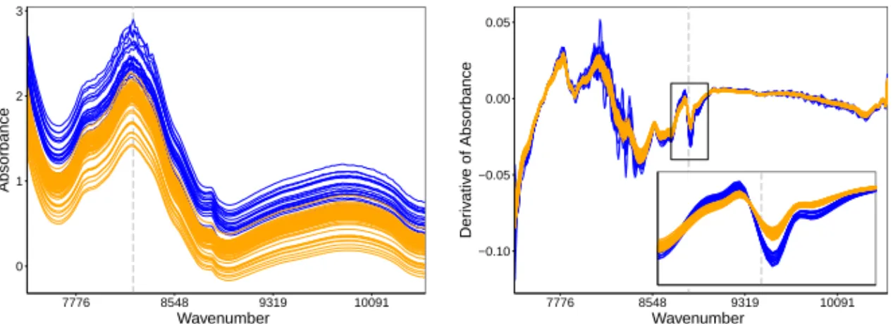
consists of near infrared spectroscopy responses for a batch of pills, measured at wavenumbers between 7398 cm−1and 10507 cm−1. (Note that wavenumbers are ex-pressed in units of inverse length.) They have been analyzed in Dyrby et al (2002) and can be downloaded fromhttp://www.models.kvl.dk/tablets. The full data set consists of tablets of different sizes and different amounts of the active ingredients. We select the 70 observations corresponding to tablets weighing 90 mg (shown in or-ange) and add 20 randomly selected observations of the tablets weighing 250 mg (in purple). These two groups of tablets also differ in the amount of active components they contain. In the main group of the 90 mg tablets, we note that the lowest curves are very similar to the others but display a downward shift, hence we can classify them as shift outliers. The 250 mg tablets show an upward shift but they are also more wiggly around wavenumber 8224. This difference becomes more pronounced when we consider the first derivatives of the curves in Figure 3. We now see that the blue curves have a different shape around wavenumber 8900. Compared to the main group of the 90 mg tablets we can consider the 250 mg tablets asshape outliers, i.e. curves whose shape differs from the majority without necessarily standing out at any time point. 0 1 2 3 7776 8548 9319 10091 Wavenumber Absorbance
Fig. 2 The tablets data with the 90 mg tablets col-ored orange and the 250 mg tablets colcol-ored purple.
−0.10 −0.05 0.00 0.05 7776 8548 9319 10091 Wavenumber Der iv ativ e of Absorbance
Fig. 3 Derivatives of the tablet curves, with the same color coding.
Another possibility is that a functional observation is outlying in anamplitude
sense, i.e. the curve may have the same shape as the majority but its scale (range, amplitude) differs. This type of outlyingness is typically found in periodic processes. An example of an amplitude outlier will be discussed in Section 2.2.
Of course it will often happen that an abnormal curve exhibits a combination of outlying behavior. It can e.g. have several spikes in the first half of the domain, and a persistent outlying behavior in the second half. Or it can be shape outlying on one part of the domain and shift outlying on another.
Often functional data are preprocessed with a baseline correction, a warping pro-cedure or other techniques, see for example Ramsay and Li (1998) and Wang and Gasser (1997). As a result it might happen that an outlying curve is transformed into a regular one. Baseline corrections will for example typically transform shift outliers into regular observations. In this case it can be useful to apply outlier detection
tech-niques to the curves defining the transformation (such as the warping functions) or to include these curves in the analysis. This will be illustrated on the tablets data in Section 5.
2.2 Functional outlier detection
All examples shown so far are univariate functional data, for which outliers can often be detected just by looking at the curves. Automatic detection of isolated and shift outliers can then easily be carried out with standard outlier detection methods for uni-variate data applied to the measurements at each time point. For shape and amplitude outliers more advanced techniques are needed, such as those mentioned in Section 1. For multivariate functional data the problem is much harder. None of the outliers de-fined in Section 2.1 will necessarily be outlying in one of the marginals, hence it is not sufficient to analyze the components separately. An example is presented in L´opez-Pintado et al (2014) where height and weight curves for boys separately do not show any marginal outlier, but a bivariate analysis flags one unusual infant. This illustrates that the correlation structure between the components should not be ignored. See also Hubert et al (2012) for other examples.
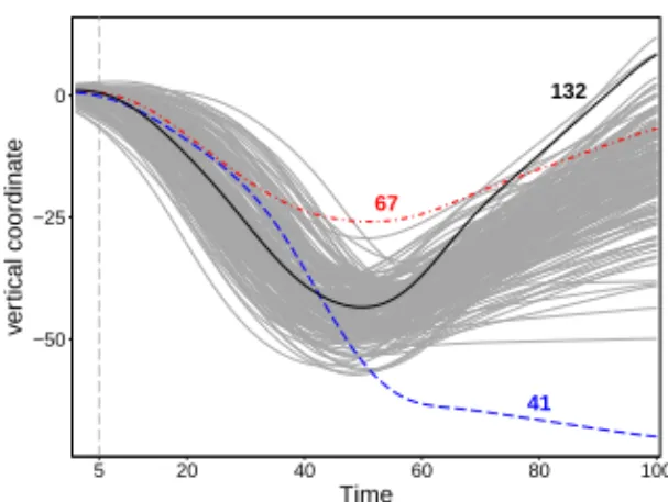
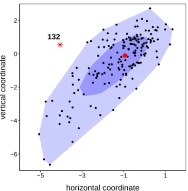
We illustrate this issue on the bivariate writing data which is a part of the Char-acter Trajectories data set included in the UCI machine learning repository (Bache and Lichman, 2013). The data measure the horizontal and vertical coordinates of a pen tip while a person writes the letter ‘i’ (without the dot)n=174 times. The ob-served data were first interpolated to obtainT=100 equally spaced time points. The resulting bivariate functional observations are displayed in Figure 4 for the horizontal coordinates and in Figure 5 for the vertical ones. When we plot both coordinates as in Figure 6 the character ‘i’ is clearly visible, but this representation does not show the speed of writing. We highlighted three outlying curves with different behavior on all three figures. The dot-dashed red curve (case 67) roughly has the same shape as the regular curves, but it has a smaller scale. This curve can be classified as an amplitude outlier. The dashed blue observation (curve 41) deviates from most of the trajectories during a long period, especially in the vertical component. This is an example of a shape outlier, which stands out in one component during a substantial time period. Yet another shape outlier is the solid black curve 132. This curve does not stand out in the marginals but it is a multivariate outlier during a long time period. To illustrate this, Figure 7 shows a bivariate scatterplot of the coordinates att=5. On this plot we see that trajectory 132 deviates from the other curves.
To detect outliers in functional data and classify them according to our taxonomy we will propose several approaches. By analogy with the non-functional case, we will first estimate the central tendency of the curves using a method which is robust to outliers. To this end we will use the multivariate functional median based on depth. Then we will construct an appropriate distance to compute the deviation of the curves from this center.
67 41 132 −20 0 20 40 20 40 60 80 100 5 Time hor iz ontal coordinate
Fig. 4 Time profile of the horizontal coordinate of the writing data set.
67 41 132 −50 −25 0 20 40 60 80 100 5 Time v er tical coordinate
Fig. 5Time profile of the vertical coordinate of the writing data set.
67 41 132 −50 −25 0 −20 0 20 40 horizontal coordinate v er tical coordinate
Fig. 6 Trajectories of the writing data set.
67 41 132 −6 −4 −2 0 2 −5 −3 −1 1 horizontal coordinate v er tical coordinate
Fig. 7 Cross-sectional scatterplot of the writing data set at time point 5.
3 Outlier detection based on halfspace depth
3.1 Multivariate (functional) halfspace depth
To measure the centrality of a point relative to a multivariate sample, Tukey (1977) introduced the halfspace depth. For simplicity of notation, we provide the definition in the population setting. LetY be a random variable onRp with distributionPY,
then the halfspace depth of any pointx∈Rprelative toPY is defined as the minimal
probability mass contained in a closed halfspace with boundary throughx: HD(x;PY) = inf
||v||=1 PY
v0Y>v0x .
Halfspace depth satisfies the requirements of a statistical depth function, as defined by Zuo and Serfling (2000a): it is affine invariant, attains its maximum value at the center of symmetry if there is one, is monotone decreasing along rays emanating from the center and vanishes at infinity. For any statistical depth functionDand for
anyα∈[0,1]theα-depth region Dαcontains the points whose depth is at leastα:
Dα={x∈Rp; D(x;PY)>α}. (1)
The boundary ofDα is known as theα-depth contour. The halfspace depth regions are closed, convex and nested for increasingα. The halfspace median (or Tukey me-dian) is defined as the center of gravity of the smallest non-empty depth region, i.e. the region containing the points with maximal halfspace depth. The finite-sample def-initions of the halfspace depth, the Tukey median and the depth regions are obtained by replacingPY by the empirical probability distributionPn.
Properties of halfspace depth have been studied extensively. Donoho and Gasko (1992) derived many finite-sample properties, including the breakdown value of the Tukey median, whereas Romanazzi (2001) derived the influence function of the half-space depth. Mass´e and Theodorescu (1994) and Rousseeuw and Ruts (1999) stud-ied several properties of the depth and the depth contours at the population level. The asymptotic distribution of the Tukey median was given in Bai and He (1999), whereas He and Wang (1997) and Zuo and Serfling (2000c) studied the convergence of the depth regions and the contours. Continuity of the depth contours and the Tukey median was investigated in Mizera and Volauf (2002). Struyf and Rousseeuw (1999) showed that the halfspace depth function of a sample completely characterizes its empirical distribution, and this was later extended to the population case.
To compute the halfspace depth, several affine invariant algorithms have been developed. Exact algorithms in two and three dimensions and an approximate al-gorithm in higher dimensions have been proposed by Rousseeuw and Ruts (1996) and Rousseeuw and Struyf (1998). Recently Liu and Zuo (2014) proposed exact al-gorithms which are feasible up to p=5. Algorithms to compute the halfspace me-dian have been developed by Rousseeuw and Ruts (1998) and Struyf and Rousseeuw (2000). To compute the depth contours the algorithm of Ruts and Rousseeuw (1996) can be used in the bivariate setting, whereas the algorithms developed in Hallin et al (2010) and Paindavaine and ˇSiman (2012) extend their applicability to at leastp=5. The bagplot (Rousseeuw et al, 1999) generalizes the univariate boxplot to bi-variate data. As an example, Figure 8 shows the bagplot of the writing data at time
t=5. Thebagis the smallestDαwhich contains 50% of the data points, and is dark-colored. The halfspace median is plotted as a red diamond. Thefence, which itself is never drawn, is obtained by inflating the bag by a factor 3 relative to the median, and the data points outside of it are flagged as outliers and plotted as stars. The light-coloredloopis the convex hull of the points inside the fence. This bagplot has the nice property not to depend on any symmetry assumption: it works just as well for skewed data. That is, the bag need not be elliptically shaped and the median need not be positioned in the middle of the bag. In Figure 8 we see a moderate deviation from symmetry.
With the rise of functional data the notion of depth has been extended to this more complex situation. For univariate functional data the first proposals include the integrated depth of Fraiman and Muniz (2001), theh-modal depth of Cuevas et al (2006) and the random projection depth (Cuevas et al, 2007). The latter could also be applied to bivariate functional data. Later L´opez-Pintado and Romo (2009, 2011) defined the (modified) band depth and the (modified) epigraph index. Recently the
132 −6 −4 −2 0 2 −5 −3 −1 1 horizontal coordinate v er tical coordinate
Fig. 8 Bagplot of the bivariate writing data at timet=5.
band depth was extended to multivariate functional data by Ieva and Paganoni (2013) and L´opez-Pintado et al (2014). The latter approach can be seen as a particular case of the multivariate functional depth introduced and studied by Claeskens et al (2014). We consider the observed curves as a realization of ap-variate stochastic process {Y(t),t∈U} onRpwithU= [a,b]. We assume that it generates continuous paths inC(U)p, the space of continuous functions fromU to Rp. Following Claeskens et al (2014), withDa statistical depth function onRpandwa function onU which integrates to one, the Multivariate Functional Depth (MFD) of a curveX∈C(U)p
with respect to the distributionPY is defined as
MFD(X;PY) = Z
U
D(X(t);PY(t))w(t)dt. (2)
wherePY(t)is the distribution ofYat timet. The MFD thus combines the local depths
at each time point. By incorporating a weight functionw(t)one can emphasize or downweight certain time regions. Similarly to the multivariate setting, the functional medianΘ(t)is defined as the curve with maximal MFD. The multivariate functional
halfspace depth (MFHD) is obtained by taking the halfspace depth as the underlying depth function in (2). Properties of MFD, MFHD and the resulting medians have been studied by Claeskens et al (2014). In particular, if the multivariate depthDhas a unique maximum at each time point, sayθ(t), then the MFD medianΘ(t)equals θ(t)and the curve is continuous.
For a functional data sample(Y1, . . . ,Yn)measured at (not necessarily equidistant)
time pointst1, . . . ,tT the finite-sample MFD of a curveXis given by
MFDn(X;Pn) = T
∑
j=1 D(X(tj);Pn(tj))Wj (3) withWj=R (tj+tj+1)/2 (tj−1+tj)/2w(t)dt (andt0=t1,tT+1=tT) andPn(tj)the empirical
distri-bution of the observed curves at timetj. For simplicity a uniform weight function will
be used throughout this paper.
Since depth functions give an outward-center ordering, we expect that outliers will have a low depth value. The ‘vanishing at infinity property’ of a statistical depth function ensures that an observation will receive zero depth when it moves away from the center. The same holds for the MFD when the curve goes to infinity at almost all time points in the domain. Simulations in Claeskens et al (2014) have illustrated that several types of outliers, among which shifted outliers, indeed obtain a low MFHD depth. So it seems natural to use functional depth values for outlier detection. This was the underlying idea in Febrero-Bande et al (2008) where critical values were derived in a nonparametric way. A parametric approach was considered in Dang and Serfling (2010) but requires knowledge about the data distribution.
However, the depth values alone do not always provide sufficient information for outlier detection. First of all, not all observations with a low depth are indeed outly-ing. For example, observations on the boundary of the convex hull of a multivariate sample only have depth 1/n. In the functional setting the problem is even more chal-lenging. In particular, isolated outliers will be very hard to detect using the MFD alone, as they will have a small multivariate depth value in only a small part of the domain. For instance, the hugely outlying curve 37 in Figure 1 has an MFHD value of 0.0973 while 5 of the 40 observations have a lower MFHD value.
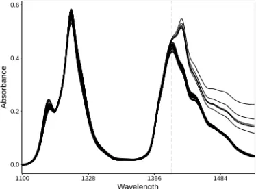
Additional insight can be obtained by looking at the values of the depth at each time point. We illustrate this on the Octane data set consisting of 39 near infrared (NIR) spectra of gasoline samples (Esbensen, 2001; Rousseeuw et al, 2006). It is known that observations 25, 26 and 36-39 have a very different spectrum as they contain added ethanol, which is required in some states. Figure 9 clearly shows the six shape outliers, which are persistently outlying from wavelength 1390 onward.
When we order the spectra according to their MFHD, the six outliers have ranks 16, 3, 12, 10, 5 and 15 respectively, hence they do not have the lowest functional depth. On the other hand spectrum 34 has the smallest depth since most of the time it lies near the lower edge of the regular data. Let us also look at the cross-sectional depth values by constructing a heatmap withn rows andT columns. Each cell of this map is colored according to HD(Yi(tj))fori=1, . . . ,nandj=1, . . . ,T, with the
smallest depth value shown as white and the overall highest depth value colored dark green. On the vertical axis we rank the curves from top to bottom according to their MFHD value, thereby putting the deepest curve at the bottom. The color of the cell on theith row and the jth column thus shows the halfspace depth at timetj of the
curve withith smallest MFHD. This yields thehalfspace depth heatmapin Figure 10.
0.0 0.2 0.4 0.6 1100 1228 1356 1484 Wavelength Absorbance
Fig. 9 Octane data set with 6 shape outliers.
11 1 2 21 33 32 20 22 16 28 18 3 24 29 27 19 13 8 7 31 10 30 17 25 39 5 9 36 4 37 12 14 35 15 38 6 26 23 34 1100 1164 1228 1292 1356 1420 1484 1548
wavelength
0.1 0.2 0.3 0.4 0.5 HDFig. 10 Halfspace depth heatmap of the octane data.
Even with the HD heatmap it is still not easy to flag the outlying curves. We note several light regions in the heatmap, but they are scattered over many rows (curves) while some of the outliers (e.g. curve 25) even have a higher HD at the higher wave-lengths than some of the regular curves. This is of course caused by the nature of halfspace depth whichranksthe data from the outside inwards without considering their distancefrom the median. When the focus is on outlier detection, including a distance-based ranking is thus indispensable. This motivates the construction of a distance measure based on halfspace depth.
3.2 The bagdistance
We first define a new statistical distance from a multivariate pointx∈Rpto a random variableY, based on the halfspace depth. This distance uses both the center and the dispersion ofY. As in the bagplot we define thebag Bas the 50% central region. This is the smallest depth region with at least 50% probability mass, i.e.B=Dα˜ with
PY(B)>0.5, andPY(Dα)<0.5 for allα>α˜. Next, we consider the ray from the halfspace medianθthroughx, and we definec(x):=cxas the intersection of this ray
and the boundary ofB. ThebagdistanceofxtoY is then given by the ratio between the Euclidean distance ofxto the halfspace median and the Euclidean distance ofcx
to the halfspace median:
bd(x;PY) =
kx−θk
kcx−θk. (4)
The denominator in (4) accounts for the dispersion ofY in the direction ofx. It is obvious that the bagdistance does not assume symmetry and is affine invariant.
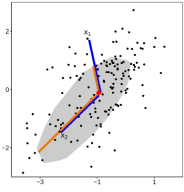
x1 x2 −2 0 2 −3 −1 1
Fig. 11 Illustration of the bagdistance between an arbitrary point and a multivariate sample.
The finite-sample definition is similar and is illustrated in Figure 11. The gray colored bag is the smallest depth region that covers half of the sample points. For two pointsx1andx2their Euclidean distance to the halfspace median (red diamond) is marked with a dark blue line, whereas the orange lines correspond to the denominator of (4) and reflect how these distances are scaled differently. Whereas the lengths of the blue lines are the same, the bagdistance ofx1is 2.01 and that ofx2is only 0.63. These values reflect the position of the points relative to the sample, one lying somewhat away from the most central half of the data and the other lying well within the central
part. Note that the bagdistance is implicitly used in the bagplot, as the fence consists of the points whose bagdistance is at most 3. Also note that the bagdistance is a very different notion from the halfspace-outlyingnessOH(x;PY) =1−2HD(x;PY)
defined by Dang and Serfling (2010). The OH contains exactly the same ranking
information as HD and is not very helpful for outlier detection either, as noted by the authors.
To compute the bagdistance of a point xwith respect to a p-variate sample we can indeed compute the bag and then the intersection pointcx. In small dimensions
computing the bag is feasible, and it is worth the effort if the bagdistance needs to be computed for many points. In higher dimensions computing the bag is hard, and then a simpler and faster algorithm is to search for the multivariate pointc∗on the ray fromθthroughxsuch that
HD(c∗;Pn) =median
i {HD(xi;Pn)}.
Since HD is monotone decreasing on the ray this is fairly fast, e.g. by means of the bisection algorithm.
When applied to elliptically symmetric distributions, the bagdistance is propor-tional to the Mahalanobis distance:
Theorem 1 If PY is an elliptically symmetric distribution with centerµand shape
matrixΣ, i.e. fY(y)∼ |Σ|−1/2h((x−µ)0Σ−1(x−µ))for some nonnegative function
h, then bd(x;PY) =k
p
(x−µ)0Σ−1(x−µ)for some constant k.
Proof We first note that under elliptical symmetry the halfspace median equals µ. Next it is well-known that the halfspace depth regions are ellipsoidsDα ={x; (x−
µ)0Σ−1(x−µ)6kα}for some constantkα depending onα, see e.g. Mass´e (2004), from which the result follows.
The bagdistance can be used to construct a metric on the spaceRpin the following way. Assume that the halfspace median is contained in the interior of the bag, that is, there exists a ball of radiusε>0 with centerθ which lies entirely inside the bag. Then define the function
g:Rp→Rp:x7→g(x) =
0 ifx=θ
(x−θ)/||cx−θ|| elsewhere
withcxas in (4). The functiongis well-defined since our assumption implies that
||cx−θ||>0 for everyx6=θ. Now define the bagdistance between two arbitrary
points as
bd(x1,x2) =||g(x1)−g(x2)||. (5)
Theorem 2 If the halfspace medianθ of a distribution P lies in the interior of the
bag, the bagdistance(5)is a metric onRp.
Proof It is clear thatbd(x1,x2)is well-defined and symmetric in its arguments. The triangle inequality follows readily from the triangle inequality for the Euclidean dis-tance. Finally we note thatbd(x1,x2) =0 impliesg(x1) =g(x2). Since the multivari-ate pointsg(x1)andg(x2)have the same direction it follows thatcx1=cx2 implying
This result continues to hold in the finite-sample case. We can also extend the bagdistance to the functional setting. Thefunctional bagdistanceof a curve to (the distribution of) a stochastic processY is defined as
f bd(X;PY) = Z
U
bd(X(t);PY(t))dt. (6)
Note that in general it is possible that this distance becomes infinite.
As in the multivariate setting, the functional bagdistance can be extended to a distance between two arbitrary continuous functionsX1andX2using the formula
f bd(X1,X2) = Z
U
bd(X1(t),X2(t))dt. (7) Under some weak conditions this is a metric:
Theorem 3 Assume Y generates continuous paths in C(U)psuch that
m:=inf
t∈Uxinf∈Rp
||cx−Θ(t)||>0 (8)
withΘ(t)the MFHD median. Then the functional bagdistance (7) is a metric on
C(U)p.
Proof Condition (8) implies that the bagdistance is defined for everyt∈U. Without loss of generality we assume thatΘ(t) =0. SinceX1,X2∈C(U)pandUis compact, it follows for allt∈Uthat||X1(t)−X2(t)||6||X1(t)||+||X2(t)||6Mfor someM<∞. Therefore f bd(X1,X2) = Z U bd(X1(t),X2(t))dt= Z U dE X1(t) ||cX1(t)|| , X2(t) ||cX2(t)|| ! dt 6 Z U ||X1(t)|| m + ||X2(t)|| m dt62 Z U M mdt.
SinceU is compact the latter integral is finite. Clearly f bd is symmetric and the triangle inequality holds. Finally f bd(X1,X2) =0 implies thatbd(X1(t),X2(t)) =0 for almost every time point sincebdis positive. This in turn implies thatX1(t) =X2(t) at almost every time point, and since they are continuous,X1=X2.
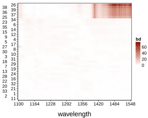
The multivariate and functional bagdistance now allow us to construct a diagnos-tic plot which shows the global outlyingness of the curve as well as the local outly-ingness at each time point. We again construct a heatmap, where now we color the cells of each row according to the cross-sectional bagdistance of the corresponding curve. The rows are sorted in decreasing order of their functional bagdistance, so that the outliers should typically be on top (as in the depth heatmap). The color of the cell on theith row and the jth column thus corresponds to the bagdistance at timetj of
the curve withith largest functional bagdistance. To emphasize that this plot focuses on theoutlyingnessof curves we use red tints. The depth heatmap of Section 3.1 used green tints instead, as it shows the degree ofcentrality.
The bagdistance heatmap of the octane data set in Figure 12 now clearly flags the six outliers. They have the highest functional bagdistance, and they become outlying from the same time point onward.
11 2 1 33 21 20 32 22 16 28 24 13 19 7 29 18 31 3 10 30 8 27 17 5 4 9 12 15 14 35 6 23 34 25 37 36 39 38 26 1100 1164 1228 1292 1356 1420 1484 1548
wavelength
0 20 40 60 bdFig. 12 Bagdistance heatmap of the octane data set.
4 Outlier detection based on adjusted outlyingness
4.1 Skew-adjusted projection depth
As an alternative to the HD based heatmaps, we also construct diagnostic plots based on a different depth function. Since the introduction of halfspace depth various other affine invariant depth functions have been defined, among which simplicial depth (Liu, 1990) and projection depth (Zuo, 2003) which is essentially the inverse of the Stahel-Donoho outlyingness (SDO). An overview of depth functions can be found in Mosler (2013). The SDO is based on the geometrical insight that a multivariate outlier should be outlying in at least one direction. The idea is to project the data onto many lines and to use a robust univariate measure of outlyingness on the projections (Stahel, 1981; Donoho, 1982). The population SDO of an arbitrary pointxwith respect to a random variableY with distributionPY is defined as
SDO(x;PY) = inf
||v||=1
|v0x−median(v0Y)| MAD(v0Y) from which the projection depth is derived:
PD(x;PY) =
1 1+SDO(x;PY)
. (9)
Since the SDO has an absolute deviation in the numerator and uses the MAD in its denominator it is best suited for symmetric distributions. For asymmetric distribu-tions Brys et al (2005) proposed the adjusted outlyingness (AO) in the context of
robust independent component analysis. The AO uses the medcouple (MC) of (Brys et al, 2004) as a robust measure of skewness. The medcouple of a univariate dataset {z1, . . . ,zn}is defined as MC(z1, . . . ,zn) =median i,j (zj−mediankzk)−(zi−mediankzk) zj−zi (10) whereiandjhave to satisfyzi6mediank(zk)6zjandzi6=zj. Note that−1<MC<
1 and MC=0 for symmetric distributions, whereas MC>0 indicates right skewness and MC<0 indicates left skewness.
The adjusted outlyingness AO is defined as:
AO(x;PY) = sup ||v||=1 v0x−median(v0Y) w2(v0Y)−median(v0Y) ifv0x>median(v0Y) median(v0Y)−v0x median(v0Y)−w1(v0Y) ifv 0x<median(v0Y) (11) where w1(Z) =Q1(Z)−1.5e−4MC(Z)IQR(Z) w2(Z) =Q3(Z) +1.5e+3MC(Z)IQR(Z)
if MC(Z)>0, whereQ1(Z)andQ3(Z)denote the first and third quartile of a univari-ate random variableZ, and IQR(Z) =Q3(Z)−Q1(Z). If MC(v0Y)<0, we replace
vby−v. The denominator of (11) corresponds to the whiskers of the univariate ad-justed boxplot proposed by Hubert and Vandervieren (2008). Other applications of the AO were studied by Hubert and Van der Veeken (2008, 2010).
We now define theskew-adjusted projection depth(SPD) as SPD(x;PY) =
1 1+AO(x;PY)
. (12)
Theorem 4 LetP be the set of all probability distribution functions onRp. The
mapping D(·,·):Rp×P →R:(x,P)7→SPD(x,P)is a statistical depth function
according to Definition 2.1 of Zuo and Serfling (2000a) and its depth regions are convex.
Proof It is clear thatD(·,·)is bounded and non-negative. Since AO is affine invariant, the skew-adjusted projection depth will be so as well. It is further evident that SPD vanishes at infinity. Note that being anH-symmetric distribution about a unique point
θ ∈Rp is equivalent to saying that median(v0Y) =v0θ for any unit vectorv∈Rp (Zuo and Serfling, 2000b). Maximality at the center and monotonicity relative to the deepest point follow immediately.
The convexity of the depth regions follows from the convexity of the adjusted out-lyingness function AO(·;P). For univariate data, the AO is a piecewise linear function composed of a downward sloping line ending in the point(median(P),0)and an up-ward sloping line starting in the same point, so it is convex. For multivariate data, the AO relative to a single directionvis thus convex too. Therefore the multivariate AO is a supremum (over allv) of convex functions.
To compute the finite-sample SPD we have to rely on approximate algorithms as it is infeasible to consider all directionsv. A convenient affine invariant procedure is obtained by considering directionsvwhich are orthogonal to an affine hyperplane through p+1 randomly drawn data points. In our implementation we use 250p di-rections.
Since the SPD is a bona fide depth function, we can plug it into (2) yielding the multivariate functional skew-adjusted projection depth (MFSPD). The MFSPD therefore satisfies the properties in Claeskens et al (2014). In particular, the resulting median is continuous when at each time point the multivariate depthDhas a unique maximum.
On the other hand we can also integrate the AO itself, yielding thefunctional adjusted outlyingness
FAO(x;PY) = Z
U
AO(X(t);PY(t))dt. (13)
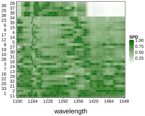
Throughout this paper we will use the skewness-adjusted AO and SPD and their functional versions instead of the original SDO and PD, because the new tools can deal with symmetric as well as asymmetric data, and they have the same good proper-ties. This is a kind of ‘insurance policy’ against skewness. As suggested by a referee, we could easily monitor the amount of skewness over time, for instance by plotting the largest absolute value of the medcouple encountered in the computation at each time point. 11 1 2 33 21 20 32 22 29 18 13 7 24 3 16 28 31 10 30 19 27 8 5 12 14 17 4 9 15 6 35 23 34 39 36 25 37 38 26 1100 1164 1228 1292 1356 1420 1484 1548
wavelength
0.25 0.50 0.75 1.00 SPDSimilar to the heatmaps based on halfspace depth and the bagdistance we can construct the skew-adjusted projection depth heatmap and the adjusted outlyingness heatmap. The SPD heatmap of the octane data is shown in Figure 13. The six outliers are now clearly identifiable. In this example the outliers also have the lowest MFSPD, as they have a high AO over a rather long period.
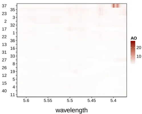
The AO heatmap of the wine data is shown in Figure 14. Instead of showing all 40 rows of the heatmap, which would make the labels harder to read, we have zoomed in on the top 24 rows. Curve 37 jumps out immediately, as the two peaks we clearly saw in the raw data are dark colored. To make the details of the other curves more visible, we also display the same heatmap by setting the colors of curve 37 to white, and rescaling the colors of the other cells. The result is in Figure 15. We now also see the wiggly behavior of several curves.
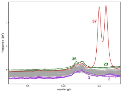
Let us now take a closer look at the curves 35, 23, 3, and 2 which are at the top of the heatmap. Curves 35 and 23 show increased cross-sectional outlyingness around wavelengths 5.37, 5.43 and 5.50. At other wavelengths these spectra have almost constant outlyingness. In Figure 16 we see that they are mild shift outliers. Curves 2 and 3 have an even more stable adjusted outlyingness profile. They can be recognized as the bottom curves in Figure 16.
4.2 Centrality-stability plot
The relation (12) between SPD and AO will allow us to construct another diagnostic plot. We start by rewriting the MFSPDnof a curveXas
MFSPDn(X;Pn) = T
∑
j=1 SPDn(X(tj);Pn(tj))Wj = T∑
j=1 1 (1+AO(X(tj);Pn(tj))W−1j =T hmean j (1+AO(X(tj);Pn(tj))Wj−1 −1where we use the abbreviation hmeanj for the harmonic mean over j=1, . . . ,T.
The MFSPD can thus be seen as the inverse of the harmonic mean of the weighted adjusted outlyingness in cross-sections. When we make a scatterplot of
MFSPDn(Yi;Pn); ave j (1+AO(Yi(tj);Pn(tj))Wj−1 (14) for alli=1, . . . ,n, the points are bounded from below by the functionz→ T
z since
the arithmetic mean is always larger than or equal to the harmonic mean.
This scatterplot is shown in Figure 17 for the octane data and in Figure 18 for the wine data. The red curve is the theoretical lower bound. We see in both examples that the outliers stand out very clearly on the vertical axis. To understand this behavior, we reconsider the relation between the hmean and the arithmetic mean of a set of positive values. These means can only be equal if all values coincide. Therefore a
11 40 4 15 5 12 19 26 8 27 33 31 16 13 36 22 1 17 32 2 3 23 35 37 5.6 5.55 5.5 5.45 5.4
wavelength
10 20 AOFig. 14 Adjusted outlyingness (AO) heatmap of the wine data (top 24 rows).
11 40 4 15 5 12 19 26 8 27 33 31 16 13 36 22 1 17 32 2 3 23 35 37 5.6 5.55 5.5 5.45 5.4
wavelength
1 2 3 4 5 6 AO2 3 23 35 37 0 1 2 5.5 5.45 5.4 wavelength Response (10 5)
Fig. 16 Wine data with some curves showing outlying behavior.
26 25 36 37 38 39 1000 2000 3000 0.4 0.6 0.8 1.0 MFSPD
Fig. 17 Scatterplot of (14) for the octane data.
2 3 23 35 37 400 600 800 1000 0.5 0.7 0.9 MFSPD
Fig. 18 Scatterplot of (14) for the wine data.
curve would be represented by a point on the lower bound if and only if its AO values would be constant over time. The vertical deviation from the lower bound thus reflects the variability of the degree of outlyingness over time.
Finally we construct thecentrality-stabilityplot as the scatterplot of 1−MFSPDn(Yi;Pn); ave j (1+AO(Yi(tj);Pn(tj))Wj−1 − T MFSPDn(Yi;Pn)
for alli=1, . . . ,n. The horizontal axis thus measures a curve’s overall deviation from centrality, and the vertical axis its AO’s deviation from stability. The deepest curves will lie in the left part of the plot, while the less central ones are to the right. Typically an isolated outlier will be in the upper region, as it is well-known that the arithmetic mean of positive numbers is more sensitive to outlying values than the harmonic mean. We expect shift outliers in the lower right region of this diagnostic plot (as they have a rather constant AO) and shape/amplitude outliers in the upper right region.
Figure 19 shows the centrality-stability plot of the wine data. The isolated out-lier 37 is again very visible. This curve is not very central either, as also outside of the two peaks it is in the outskirts of the curves. Curves 2, 3, 23 and 35 are at the
2 3 23 35 37 0 100 200 300 0.0 0.1 0.2 0.3 0.4 0.5 1−MFSPD V er tical distance
Fig. 19 Centrality-stability plot of the wine data.
bottom right of the plot. We already noted in Figure 16 that curves 2 and 3 have sta-ble adjusted outlyingness profiles across wavelengths. This is confirmed by their low vertical coordinates in the centrality-stability plot.
5 Real data analysis
Whereas the examples in Sections 3 and 4 were univariate functional data sets, we now apply our new methodology to two multivariate data sets.
5.1 Writing data
The writing data were introduced in Subsection 2.2, where we also described the out-lying behavior of some of the curves (41, 67 and 132). The centrality-stability plot of this bivariate functional data set is shown in Figure 20, the trajectories are displayed in Figure 21 and their marginals in Figures 22 and 23. In the centrality-stability plot observations 41 and 132 indeed stand out. The MFSPD depth of the blue curve 41 is not extremely small (as seen on the horizontal axis of the centrality-stability plot), but its outlyingness is quite variable, resulting in a high vertical coordinate in Figure 20.
The solid black curve 132 has the lowest MFSPD although it does not look very outlying in the marginals, but it is outlying in the multivariate sense as we saw in Fig-ures 7 and 8. From its vertical coordinate in the centrality-stability plot we conclude that the cross-sectional outlyingness does vary somewhat over time. The dot-dashed red curve 67 is in the outskirts of the data judging from its MFSPD on the horizontal axis in Figure 20, and its vertical position in that plot tells us that its AO values are quite variable. Curves 30 (dashed green), 95 (solid purple) and 121 (dot-dashed or-ange) are even higher in the centrality-stability plot, and we see that they are mostly outlying in the right hand side of Figure 21.
30 41 67 95 121 132 0 10 20 30 40 50 0.2 0.4 0.6 1−MFSPD V er tical distance
Fig. 20 Centrality-stability plot of the writing data.
30 41 67 95 121 132 −50 −25 0 −20 0 20 40 horizontal coordinate v er tical coordinate
Fig. 21 Writing data with some outliers colored.
30 41 67 95 121 132 −20 0 20 40 20 40 60 80 100 Time hor iz ontal coordinate
Fig. 22 Horizontal coordinate of the writing data with some outliers colored.
30 41 67 95 121 132 −50 −25 0 20 40 60 80 100 Time v er tical coordinate
Fig. 23 Vertical coordinate of the writing data with some outliers colored.
5.2 Tablets Data
As explained in Subsection 2.1 the tablets data consists of two groups of pills, and the data contains shift outliers and shape outliers. A common practice in chemometrics is to first apply a baseline correction, so from each curve we subtract its mean (over all wavenumbers). These baseline corrections are constant functions shown in Figure 24. The corrected spectra are displayed in Figure 25. From this plot it can already be seen that the lower curves (the shift outliers) are transformed to regular curves. If we do not want to lose the information that some of the curves were outlying prior to the preprocessing step, we can include the baseline functions in our analysis. Moreover, to increase the potential of finding shape outliers, we include the derivatives of the curves (shown in Figure 3) as well. All together we thus perform our analysis on a three-dimensional functional data set.
First we look at the SPD heatmap in Figure 26 and the AO heatmap in Figure 27. Both show the top 50 rows out of 90. These heatmaps reveal interesting structures in the data. Curves 71 through 90 show an increased cross-sectional outlyingness be-tween wavenumbers 8850 and 8950. Among the rows with the highest functional AO
0.6 0.9 1.2 1.5 7776 8548 9319 10091 Wavenumber
Base line shift
Fig. 24Baseline correction functions of the tablets data. −0.5 0.0 0.5 1.0 1.5 7776 8548 9319 10091 Wavenumber Absorbance
Fig. 25 The baseline-corrected spectra.
we also find curves 1 through 10. A similar pattern can be seen in the depth heatmap. However, there is a difference between these two groups. The cross-sectional ad-justed outlyingness of the first 10 observations is mostly stable across wavenumbers, whereas the other outliers show more variability in their AO values.
This difference becomes more explicit in the centrality-stability plot (Figure 28). We clearly distinguish three groups of observations: regular ones, curves with low depth and stable outlyingness, and those with low depth and highly variable AO val-ues. They correspond nicely to the three types of curves that could be seen on the raw data: the 90 mg pills (orange), the downward shifted 90 mg (red), and the 250 mg (purple), see Figure 29. As expected the shifted outliers have an almost constant deviation from the functional median and thus are situated in the lower right corner of the centrality-stability plot. The wiggly behavior of the 250 mg tablets causes them to be located in the upper right part.
One might wonder whether these groups could also be found by applying existing univariate outlier detection tools to the marginal curves. We first apply the functional boxplot of Sun and Genton (2011) to each of the three univariate functional data sets. On the baseline functions (Figure 24), observations 1, 2, 4-6, 71-74, 79, 83, 88 and 90 are flagged as outliers. On the baseline-corrected spectra the functional boxplot indicates tablets 1, 4, 73, 76, 79, 83 and 90 as outliers. Applied to the derivatives it flags observations 1, 4, 5, 71-84 and 87-90. Even if we combine the results from the three components, tablets 3, 7-10, 85 and 86 are not detected.
Next we apply the outliergram which has recently been proposed by Arribas-Gil and Romo (2014). It combines two univariate functional depth methods: the modified band depth (MBD) and the modified epigraph index (MEI). Arribas-Gil and Romo (2014) show that for each curve
MBD6a0+a1MEI+a2n2MEI2
witha0, a1, a2 depending on n only. Using this relation they propose to plot the depths of the observations in the(MBD,MEI)-plane. They then define shape outliers as those observations whose distancedi=a0+a1MEIi+a2n2MEI2i−MBD is flagged
39 40 36 31 43 33 35 15 21 46 17 19 41 86 11 16 14 34 75 78 12 45 84 87 80 13 85 81 8 77 74 89 82 76 72 71 88 7 10 9 73 3 79 5 6 83 2 90 4 1 7776 8548 9319 10091 Wavenumber 0.25 0.50 0.75 SPD
Fig. 26 SPD heatmap of the tablets data (top 50 rows).
47 36 31 40 15 33 43 35 46 17 19 21 41 16 11 14 12 34 86 45 75 13 78 84 87 80 8 85 81 77 74 89 7 82 10 9 71 72 76 3 88 73 6 5 79 2 83 90 1 4 7776 8548 9319 10091 Wavenumber 4 8 12 AO
100 200 300 0.4 0.5 0.6 0.7 0.8 1−MFSPD V er tical distance
Fig. 28 Centrality-stability plot of the tablets data. 0 1 2 3 7776 8548 9319 10091 Wavenumber Absorbance
Fig. 29 Raw tablet curves colored according to their type.
If we apply this technique to the marginals of our three-dimensional functional data set, no outliers are detected from the baseline functions or the baseline-corrected spectra. Figure 30 shows the outliergram (right) of the derivatives of the spectra (left). Only observation 90 is flagged as a shape outlier and is marked on the left plot. Our multivariate analysis is thus much more powerful here.
6 Conclusion and outlook
We extend the toolbox of multivariate functional data analysis by new techniques for outlier detection. Functional data can have various kinds of outlyingness. A curve can have isolated or persistent outlying behavior, and the latter can be of the shift, amplitude, or shape variety, or a combination of those. The multivariate nature of the data makes these harder to detect than in the univariate functional case.
7500 8000 8500 9000 9500 10000 −0.10 −0.05 0.00 0.05 Observations Respons 0.40 0.45 0.50 0.55 0.60 0.65 0.1 0.2 0.3 0.4 0.5 Outliergram
Modified Epigraph Index
Modified Band Depth
90
Fig. 30 Derivatives of the tablet spectra (left) and their outliergram (right). Curve 90 is shown in black in the left panel.
Our new tools are based on depth-related notions so they do not have to assume any symmetry. We introduce the bagdistance, a metric based on halfspace depth. Even in the simpler case of multivariate nonfunctional data this is a new concept. The functional bagdistance carries more numerical information than the functional halfspace depth alone, and the new bagdistance heatmap helps to distinguish between isolated and persistent outlyingness.
A second approach is to extend the well-known projection depth to skewed dis-tributions by basing it on the adjusted outlyingness (AO). In the multivariate case thisskewness-adjusted projection depth(SPD) satisfies the depth axioms of Zuo and Serfling (2000a) and has convex depth regions. Integrating the SPD over time yields the functional SPD, as well as the SPD heatmap which can reveal detailed structure in the data. Combining information from the AO with the functional SPD we obtain a new diagnostic plot, which we call thecentrality-stability plotbecause it contrasts the overall depth of a curve with the time-variability of its cross-sectional outlyingness. In the examples we illustrate the power of these multivariate functional tools, also compared to univariate analysis of the marginals.
We are currently working on a package for R and a corresponding toolbox for MATLAB implementing the techniques described in this paper. In future work we will investigate how these new tools can be used for other purposes such as supervised classification of multivariate data and of functional data.
References
Arribas-Gil A, Romo J (2014) Shape outlier detection and visualization for functional data: the outliergram. Biostatistics 15(4):603-619
Bache K, Lichman M (2013) UCI Machine Learning Repository. URL http://archive.ics.uci.edu/ml
Bai ZD, He X (1999) Asymptotic distributions of the maximal depth estimators for regression and multivariate location. The Annals of Statistics 27(5):1616–1637 Berrendero J, Justel A, Svarc M (2011) Principal components for multivariate
func-tional data. Computafunc-tional Statistics & Data Analysis 55(9):2619–2634
Brys G, Hubert M, Struyf A (2004) A robust measure of skewness. Journal of Com-putational and Graphical Statistics 13:996–1017
Brys G, Hubert M, Rousseeuw PJ (2005) A robustification of Independent Compo-nent Analysis. Journal of Chemometrics 19:364–375
Claeskens G, Hubert M, Slaets L, Vakili K (2014) Multivariate functional halfspace depth. Journal of the American Statistical Association 109(505):411–423
Cuevas A, Febrero M, Fraiman R (2006) On the use of the bootstrap for esti-mating functions with functional data. Computational Statistics & Data Analysis 51(2):1063–1074
Cuevas A, Febrero M, Fraiman R (2007) Robust estimation and classification for functional data via projection-based depth notions. Computational Statistics 22:481–496
Dang X, Serfling R (2010) Nonparametric depth-based multivariate outlier identi-fiers, and masking robustness properties. Journal of Statistical Planning and Infer-ence 140(1):198 – 213
Donoho D (1982) Breakdown properties of multivariate location estimators. PhD Qualifying paper, Dept Statistics, Harvard University, Boston
Donoho D, Gasko M (1992) Breakdown properties of location estimates based on halfspace depth and projected outlyingness. The Annals of Statistics 20(4):1803– 1827
Dyrby M, Engelsen S, Nørgaard L, Bruhn M, Lundsberg-Nielsen L (2002) Chemo-metric quantization of the active substance in a pharmaceutical tablet using near-infrared (NIR) transmittance and NIR FT-Raman spectra. Applied Spectroscopy 56(5):579–585
Esbensen K (2001) Multivariate Data Analysis in Practice, 5th edn. Camo Process AS
Febrero-Bande M, Galeano P, Gonz´alez-Manteiga W (2008) Outlier detection in functional data by depth measures, with application to identify abnormal NOx
lev-els. Environmetrics 19(4):331–345
Ferraty F, Vieu P (2006) Nonparametric Functional Data Analysis: Theory and Prac-tice. Springer, New York
Fraiman R, Muniz G (2001) Trimmed means for functional data. Test 10:419–440 Hallin M, Paindaveine D, ˇSiman M (2010) Multivariate quantiles and multiple-output
regression quantiles: from L1 optimization to halfspace depth. The Annals of Statistics 38(2):635–669
He X, Wang G (1997) Convergence of depth contours for multivariate datasets. The Annals of Statistics 25(2):495–504
Hubert M, Vandervieren E (2008) An adjusted boxplot for skewed distributions. Computational Statistics and Data Analysis 52(12):5186–5201
Hubert M, Van der Veeken S (2008) Outlier detection for skewed data. Journal of Chemometrics 22:235–246
Hubert M, Van der Veeken S (2010) Robust classification for skewed data. Advances in Data Analysis and Classification 4:239–254
Hubert M, Claeskens G, De Ketelaere B, Vakili K (2012) A new depth-based approach for detecting outlying curves. In: Colubi A, Fokianos K, Gonzalez-Rodriguez G, Kontoghiorghes E (eds) Proceedings of COMPSTAT 2012, pp 329– 340
Hyndman R (1996) Computing and graphing highest density regions. The American Statistician 50:120–126
Hyndman R, Shang H (2010) Rainbow plots, bagplots, and boxplots for functional data. Journal of Computational and Graphical Statistics 19(1):29–45
Ieva F, Paganoni AM (2013) Depth measures for multivariate functional data. Com-munications in Statistics - Theory and Methods 42(7):1265–1276
Larsen F, van den Berg F, Engelsen S (2006) An exploratory chemometric study of NMR spectra of table wines. Journal of Chemometrics 20(5):198–208
Liu R (1990) On a notion of data depth based on random simplices. The Annals of Statistics 18(1):405–414
Liu X, Zuo Y (2014) Computing halfspace depth and regression depth. Communica-tions in Statistics - Simulation and Computation 43(5):969–985
L´opez-Pintado S, Romo J (2009) On the concept of depth for functional data. Journal of the American Statistical Association 104:718–734
L´opez-Pintado S, Romo J (2011) A half-region depth for functional data. Computa-tional Statistics & Data Analysis 55:1679–1695
L´opez-Pintado S, Sun Y, Lin J, Genton M (2014) Simplicial band depth for multi-variate functional data. Advances in Data Analysis and Classification 8:321–338 Maronna R, Martin D, Yohai V (2006) Robust Statistics: Theory and Methods. Wiley,
New York
Mass´e JC (2004) Asymptotics for the Tukey depth process, with an application to a multivariate trimmed mean. Bernoulli 10(3):397–419
Mass´e JC, Theodorescu R (1994) Halfplane trimming for bivariate distributions. Journal of Multivariate Analysis 48(2):188–202
Mizera I, Volauf M (2002) Continuity of halfspace depth contours and maximum depth estimators: diagnostics of depth-related methods. Journal of Multivariate Analysis 83(2):365–388
Mosler K (2013) Depth statistics. In: Becker C, Fried R, Kuhnt S (eds) Robustness and Complex Data Structures, Festschrift in Honour of Ursula Gather, Springer, Berlin, pp 17–34
Paindavaine D, ˇSiman M (2012) Computing multiple-output regression quantile re-gions. Computational Statistics & Data Analysis 56:840–853
Pigoli D, Sangalli L (2012) Wavelets in functional data analysis: estimation of multi-dimensional curves and their derivatives. Computational Statistics & Data Analysis 56(6):1482–1498
Ramsay J, Silverman BW (2002) Applied Functional Data Analysis. Springer Series in Statistics, Springer
Ramsay J, Silverman BW (2006) Functional Data Analysis, 2nd edn. Springer, New York
Ramsay JO, Li X (1998) Curve registration. Journal of the Royal Statistical Society, Series B 60(2):351–363
Romanazzi M (2001) Influence function of halfspace depth. Journal of Multivariate Analysis 77:138–161
Rousseeuw PJ, Leroy A (1987) Robust Regression and Outlier Detection. Wiley-Interscience, New York
Rousseeuw PJ, Ruts I (1996) Bivariate location depth. Applied Statistics 45:516–526 Rousseeuw PJ, Ruts I (1998) Constructing the bivariate Tukey median. Statistica
Sinica 8:827–839
Rousseeuw PJ, Ruts I (1999) The depth function of a population distribution. Metrika 49:213–244
Rousseeuw PJ, Struyf A (1998) Computing location depth and regression depth in higher dimensions. Statistics and Computing 8:193–203
Rousseeuw PJ, Ruts I, Tukey J (1999) The bagplot: a bivariate boxplot. The American Statistician 53:382–387
Rousseeuw PJ, Debruyne M, Engelen S, Hubert M (2006) Robustness and outlier detection in chemometrics. Critical Reviews in Analytical Chemistry 36:221–242
Ruts I, Rousseeuw PJ (1996) Computing depth contours of bivariate point clouds. Computational Statistics & Data Analysis 23:153–168
Stahel W (1981) Robuste Sch¨atzungen: infinitesimale Optimalit¨at und Sch¨atzungen von Kovarianzmatrizen. PhD thesis, ETH Z¨urich
Struyf A, Rousseeuw PJ (1999) Halfspace depth and regression depth characterize the empirical distribution. Journal of Multivariate Analysis 69(1):135–153 Struyf A, Rousseeuw PJ (2000) High-dimensional computation of the deepest
loca-tion. Computational Statistics & Data Analysis 34(4):415–426
Sun Y, Genton M (2011) Functional boxplots. Journal of Computational and Graphi-cal Statistics 20(2):316–334
Tukey J (1977) Exploratory Data Analysis. Reading (Addison-Wesley), Mas-sachusetts
Wang K, Gasser T (1997) Alignment of curves by dynamic time warping. The Annals of Statistics 25(3):1251–1276
Zuo Y (2003) Projection-based depth functions and associated medians. The Annals of Statistics 31(5):1460–1490
Zuo Y, Serfling R (2000a) General notions of statistical depth function. The Annals of Statistics 28:461–482
Zuo Y, Serfling R (2000b) On the performance of some robust nonparametric lo-cation measures relative to a general notion of multivariate symmetry. Journal of Statistical Planning and Inference 84:55–79
Zuo Y, Serfling R (2000c) Structural properties and convergence results for contours of sample statistical depth functions. The Annals of Statistics 28(2):483–499