Unsupervised Representation Learning with Correlations

(1)

Unsupervised Representation Learning with Correlations

Da Tang

Submitted in partial fulfillment of the requirements for the degree of

Doctor of Philosophy

in the Graduate School of Arts and Sciences

COLUMBIA UNIVERSITY

(2)

(3)

Abstract

Unsupervised Representation Learning with Correlations Da Tang

Unsupervised representation learning algorithms have been playing important roles in ma-chine learning and related fields. However, due to optimization intractability or lack of consider-ation in given data correlconsider-ation structures, some unsupervised representconsider-ation learning algorithms still cannot well discover the inherent features from the data, under certain circumstances. This thesis extends these algorithms, and improves over the above issues by taking data correlations into consideration.

We study three different aspects of improvements on unsupervised representation learning algorithms by utilizing correlation information, via the following three tasks respectively:

1. Using estimated correlations between data points to provide smart optimization initializa-tions, for multi-way matching (Chapter 2). In this work, we define a correlation score between pairs of data points as metrics for correlations, and initialize all the permutation matrices along a maximum spanning tree of the undirected graph with these metrics as the weights. 2. Faster optimization by utilizing the correlations in the observations, for variational inference

(Chapter 3). We construct a positive definite matrix from the negative Hessian of the log-likelihood part of the objective that can capture the influence of the observation correlations on the parameter vector. We then use the inverse of this matrix to rescale the gradient. 3. Utilizing additionalside-informationon data correlation structures to explicitly learn

corre-lations between data points, for extensions of Variational Auto-Encoders (vaes) (Chapters 4 and 5). Consider the case where we know a correlation graphGof the data points. Instead

(4)

of placing ani.i.d. prior as in the most common setting, we adopt correlated priors and/or correlated variational distributions on the latent variables through utilizing the graphG. Empirical results on these tasks show the success of the proposed methods in improving the performances of unsupervised representation learning algorithms. We compare our methods with multiple recent advanced algorithms on various tasks, on both synthetic and real datasets. We also provide theoretical analysis for some of the proposed methods, showing their advantages under certain situations.

The proposed methods have wide ranges of applications. For examples, image compres-sion (via smart initializations for multi-way matching), link prediction (by

vaes

with correlations), etc.

(5)

vaes

. . . 2

1.1.2 Dictionary learning . . . 4

1.1.3 Word embeddings . . . 5

1.1.4 Permutations for bag-of-elements data . . . 6

1.2 Extensions and improvements with correlation information . . . 7

1.2.1 Estimated correlations for multi-way matching . . . 8

1.2.2 Efficient inference with pathological objectives . . . 8

1.2.3 Correlated representations with side-information . . . 9

1.3 Organization of this thesis . . . 10

1.4 Related papers . . . 10

(6)

2.1 Motivation . . . 11

2.2 Consistent matching for sets of elements . . . 13

2.3 Coordinate optimization with smart initialization . . . 15

2.3.1 Coordinate ascent over permutations . . . 16

2.3.2 MST-based initializations . . . 17

2.3.3 Analysis of the coordinate updates . . . 18

2.3.4 Practical improvements . . . 27

2.4 Experiments . . . 29

2.4.1 PCA reconstruction of MNIST digits . . . 30

2.4.2 Stereo landmark alignments . . . 31

2.4.3 Repetitive structures of key points . . . 33

2.4.4 Experiments in domains beyond computer vision . . . 34

2.5 Summary . . . 35

Chapter 3: Variational Predictive Natural Gradient . . . . 36

3.2 Related work . . . 38

3.3 Background . . . 38

3.4 The Variational Predictive Natural Gradient . . . 40

3.4.1 Negative Hessian of the expected log-likelihood . . . 41

3.4.2 Predictive sampling for positive semidefiniteness . . . 44

3.4.3 The Variational Predictive Natural Gradient . . . 46

(7)

3.5 Variational inference with approximate curvature . . . 50

3.6.1 Bayesian Logistic regression . . . 52

3.6.2 Variational Auto-Encoder . . . 53

3.6.3 Variational matrix factorization . . . 56

3.6.4 More details on the experiments . . . 58

3.7 Summary . . . 60

Chapter 4: Correlated Variational Auto-Encoders . . . . 61

4.2

cvaes

on acyclic graphs . . . 63

4.2.1 Variational Auto-Encodings . . . 63

4.2.2 Correlated priors on acyclic graphs . . . 64

4.2.3

cvaes

on acyclic graphs . . . 66

4.3

cvaes

on general graphs . . . 67

4.3.1 Why the trivial generalization fails . . . 68

4.3.2 Inference with a weighted objective . . . 69

4.3.3 Computing the subgraph weights . . . 73

4.3.4 Regularization with non-edges . . . 78

4.4.1 Experiment settings . . . 80

4.4.2 Results . . . 82

(8)

4.6 Summary . . . 87

Chapter 5: Adaptive Correlated Variational Auto-Encoders . . . . 89

5.2 Adaptive Correlated

Vaes

. . . 91

5.2.1 A non-uniform mixture prior . . . 91

5.2.2 Learning the non-uniform mixture . . . 92

5.2.3 Learning with alternating updates . . . 94

5.2.4 Exact marginal posterior approximation with belief propagation . . . 96

5.3 Experiments . . . 97 5.3.1 Experiment settings . . . 98 5.3.2 Results . . . 102 5.4 Related work . . . 107 5.5 Summary . . . 107 Conclusion . . . . 108 References . . . . 111

(9)

List of Tables

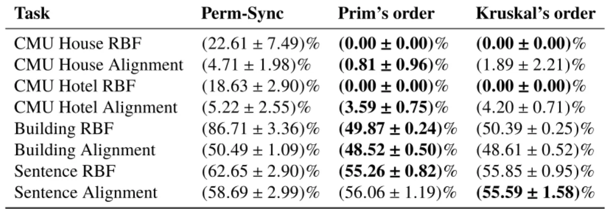
2.1 Average error rates of alignments for the datasets House, Hotel, Building and Sentence 32

3.1 Bayesian Logistic regression AUC . . . 54

4.1 Synthetic user matching test RR . . . 83

4.2 Spectral clustering normalized MI scores . . . 85

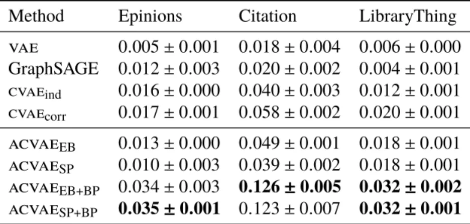
4.3 Link prediction test normalized CRR . . . 86

5.1 Link prediction normalized CRR . . . 104

5.2 Hieracrhical clustering normalized MI scores . . . 104

5.3

elbo

| average NCRR comparisons between ACVAE (with BP) on Epinions and Citation . . . 105

5.4

elbo

| average NCRR comparisons between ACVAE (without BP) and CVAE on Citation . . . 105

(10)

List of Figures

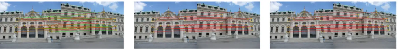
2.1 Results for the PCA reconstruction experiment . . . 30 2.2 Key points alignment for the Building dataset. Green lines are the ground-truth

alignments while red lines are the computed alignments. Less green lines being exposed means a better performance. . . 33

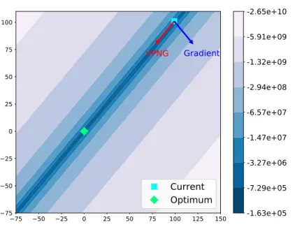
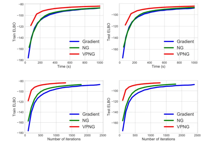
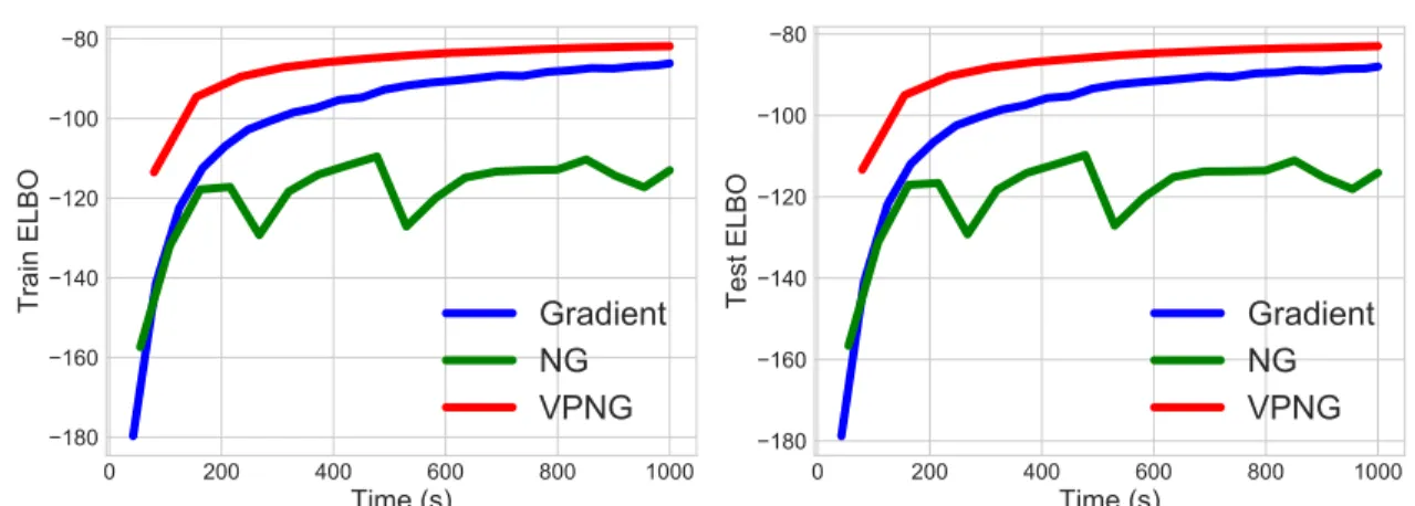
3.1 The

vpngs

are more effective than standard gradients and standard natural gradients (pointing into the same direction with the standard gradients for this example). . . 40 3.2 Bayesian Logistic regression test AUC-iteration learning curve. . . 54 3.3

Vae

learning curves on binarized MNIST . . . 55

3.4

Vmf

learning curves on MovieLens 20M . . . 57 3.5

Vae

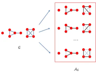
learning curves on binarized MNIST, without exponential moving averages . . 59

4.1 Visualization of the set of maximal acyclic subgraphs (right) of the given graph

G _{(left). On the right, the dark solid edges are selected and light dashed edges}

not selected. As can be seen from this figure, each subgraphG0 ∈ AG is just a combination of a spanning trees over all ofG’s connected components. In total, this graphGhas |AG| =48maximal acyclic subgraphs. . . 70

(11)

Acknowledgements

It has been a wonderful journey for me at Columbia University. It is my honor to stay here for four and a half years. I would like to thank Columbia University for giving me a great place for study and research. The academic environment here was inclusive, which helps me better pursue my research goal.

I would like to especially thank my adviser, Prof. Tony Jebara, for his professional and careful supervision. He deeply helped me on my research in various aspects. In addition to regular dis-cussions on specific research questions, he also taught me the way of exploring new research ideas. After the Ph.D. study at Columbia, I felt I have earned a big accomplishment. I can propose my own research topics and study them independently, and I am ready for exploring more in the future. Really thank Prof. Jebara for advising me to be a better researcher.

I would also like to thank my other dissertation committee members, Prof. David Blei, Prof. Daniel Hsu, Prof. John Paisley and Prof. Nicholas Ruozzi. Thank them for their professional suggestions on my thesis research. They all have provided thoughtful comments along the way of my Ph.D. study, which strongly inspired me when I met difficulties in my research. In addition, I want to especially thank Prof. David Blei here since he and his research group gave me a lot of advice and suggestions for my research.

Besides, I also want to thank my coauthors, Jianfeng Gao, Chong Wang, Lihong Li, Rajesh Ranganath, Dawen Liang, Xiujun Li, and many others. I would like to especially thank Rajesh Ranganath for his wonderful research guidance and his patience. We worked on a research project for a long time (the

vpng

work in Chapter 3). He consistently proposed insightful ideas and spent a

(12)

large amount of time together with me on this work. I also want to greatly thank Dawen Liang for his professional research insights and his encouragement. He helped me a lot in research discussions, and he gave me support when I almost gave up solving some hard questions. Really thank him for his help.

During my Ph.D. study, I have been honored to intern at Google, Microsoft and Netflix. I want to thank my mentors: Lan Nie, Sajid Siddiqi, Jianfeng Gao, Chong Wang, Lihong Li, Xiujun Li and Dawen Liang. Thank them for their professional supervision. I really enjoy my experiences at all of these companies.

At the end, with full of gratitude, I want to thank my parents for their love and consideration. Without your support, I could not have easily overcome the difficulties that I met during my Ph.D. study. I am proud to be your son.

(13)

(14)

Chapter 1: Introduction

Unsupervised representation learning [1, 2], or unsupervised feature learning, is a popular research direction in machine learning. Basically, any algorithm that learns any kind of latent representa-tions (or features) from observed data without supervision signals (e.g. the outcome variables in regression or the labels in classification) can be viewed as a kind of unsupervised representation learning methods. Since unsupervised representation learning algorithms can extract features from the data, it can automatically transform observed raw data into well-shaped data that can be used as inputs for machine learning algorithms.

The feature learning steps that unsupervised representation learning performs is important since the performance of many machine learning algorithms strongly depends on the inputs. To illustrate, let us consider a scenario where we have a movie rating vector for each userui (e.g. the MovieLens dataset [3]) . We have movie ratings of this user split into two halves and get two synthetic usersuiA

anduiB, each has half ofui’s ratings. And our task is to find theN (the number of users) one-to-one

mapping between these 2N synthetic users. Directly applying the distance metrics on the rating vectors of these synthetic users to find the mapping is not good idea since the set of movies that each pair of synthetic users have watched are almost disjoint. However, as shown in one experiment that we will see later in Section 4.4.2 of Chapter 4, applying a Variational Auto-Encoder (vae) [4, 5] to learn low dimensional representations for each synthetic users and finding the mapping based on the distance metrics on these representations performs well, as the latent representations can potentially provide essential information that the pure rating vectors cannot provide. Moreover, in natural language processing, there are many ways that we can learn word embeddings [1, 6, 7] as feature vectors for words and apply these feature vectors in machine learning algorithms, while we

(15)

have no idea on the words’ meaning from the input documents themselves if we do not perform such feature learning. Therefore, feature learning plays an important role for machine learning and it can be applied in many related fields as well.

In addition, compared to supervised representation learning algorithm methods (e.g. supervised dictionary learning [8]), unsupervised representation learning methods have the advantages that they do not need to learn from labels, which may be expensive or hard to obtain for some tasks. For example, in word embedding, we can learn useful features for the words without labels on the part-of-speech information, the parse trees, the tense or any other information of the text, while performing such kind of labeling may be hard. As a result, unsupervised representation learning methods are potentially more applicable in practice, and hence studying such methods is an inter-esting and useful topic in the machine learning community.

1.1 Existing algorithms

There are many existing unsupervised representation learning algorithms. We briefly introduce some of them here.

1.1.1 Matrix factorization, Auto-Encoders and

vaes

We consider a real application, movie recommendation with user-based collaborative filtering [9], to illustrate matrix factorization, Auto-Encoders and

vaes. Assume that we are giving a dataset

showing the ratings of movies that N usersu1, . . . ,uN have watched among M moviest1, . . . ,tM. Then this dataset forms a matrix X ∈RN×M whereXi jis the rating that the useruiproposes on the movietj. We set Xi j to be 0 if the userui has not watched the movietj.

To learn the interests of each userui, and the style (or types of contents) of each movie tj so as

to be recommended to the users, matrix factorization [10] learns a d-dimensional latent vector

(16)

and uses the inner product X˜i j = z>_i wj as the predicted value for the entry Xi j. By applying the squared Euclidean distance as the loss function and adding regularization terms on the parameter, with Z = z1 z2 . . . zN > ∈_RN×d_andW = w1 w2 . . . wM >

∈_RM×d_{as the matrix}

rep-resentations of the latent vectors, standard matrix factorization minimizes the following objective function: min Z,W L(Z,W) = X (i,j):X_{i j}_,0 kz>_i wj −Xi jk₂2+λZkZk₂2+λWkWk₂2. (1.1)

Here λZ, λW ≥ 0 are the L2-regularization parameters. We also call this method as matrix fac-torization with explicit feedback [11] since it only optimizes with the observed entries. Similarly, another type of the matrix factorization is the case with implicit feedback [11], which treats the unseen entries as zeros and optimizes on the whole matrix:

min

Z,W L(Z,W)= kZ

>

W −Xk₂2+λZkZk₂2+λWkWk₂2. (1.2)

The two objectives (Equations 1.1 and 1.2) can be viewed as a probabilistic generative model on the data matrixX, where the likelihood of the entryXi j is a Gaussian distribution with the mean equals the inner product z>i wj [12]. In fact, depending on the type of the dataset, the likelihood can also

be other distributions. For example, we can set the likelihood of Xi j to be Poisson distribution (we call this Poisson matrix factorization) when we have non-negative integer input data [11].

However, the standard matrix factorization fits data matrixX with a linear transformation from the latent variableZ(since the parameter for the likelihood on each entryXi jis just a linear transforma-tion from the latent embedding zi), which makes the model lack of expressiveness. An extension for this is to learn a non-linear mapping functiongθ : Rd → RM that maps the latent embedding

zi to the data vector xi ∈ RM for each user ui. This function gθ is parameterized by a vector θ and it is shared among all data points. On the other hand, we may also want to learn a function

fλ :RM →Rdthat maps the data vector xito the latent representation zi = fλ(xi)for each userui

(17)

get theAuto-Encoder(AE) [13, 4]: min λ,θ L(λ,θ)= n X i=1 kgθ(fλ(xi))− xik₂2. (1.3)

Here the objective minimizes the reconstruction loss of the data xi from the latent representation

zi. The two functions f andgmay seem like a pair of inverse functions, but it is not necessarily the case. Instead, Auto-Encoders just aim at learning a good mapping from the latent representations to the data, and a mapping in the reverse direction as well. In practice, to make the model more expressive, we usually choose f andgto be neural networks [13, 4] andλ,θare the parameters for these two networks, respectively,

Auto-Encoders have the two advantages over matrix factorizations. First, the vectorgθ(zi)can be a non-linear mapping on the latent embedding zi, while for matrix factorization this is just a linear mappingW>zi. Second, we have a mapping fλ that can be used to compute the latent embeddings

zifrom the data, while we need to learn a different embedding vector zi for each user xiin matrix

factorization. This technique that Auto-Encoders apply is called amortized inference, which we will discuss in more details in Chapter 4.

In Auto-Encoders, the latent embeddings zi are deterministic functions of the data xi. In fact, stochastic mappings can learn better representations as features [4]. If we extend the mapping fλ

to be stochastic, we get the Variational Auto-Encoder (vae) [4, 5], which is one of the models that this thesis mainly focuses on. It can learn stochastic latent representations for data and performs well on various tasks. We will introduce this model in detail in Chapter 4.

1.1.2 Dictionary learning

In dictionary learning and compressive sensing [14, 15], we learn a dictionary of feature vectors that can be used as a basis with which the input data can be expressed as linear combinations of these vectors with sparse coefficients. Mathematically, given a set of observed vectors y1, . . . ,yn ∈ Rm,

(18)

we would like to learn a dictionary matrix A ∈ Rm×d and a set of sparse vectors x1, . . . ,xn ∈ Rd

such that the following objective is minimized (λ >0is a regularization parameter):

min A,x1,...,xn n X i=1 (kyi−Axik₂2+λkxik0). (1.4)

Here the columns a1, . . . ,am ∈ Rd of the dictionary matrix Aare the feature vectors that we want to learn. Usually, we will have the observed vector dimensionalitym dand we hope the learned vectors xi are very sparse. In this way, dictionary learning can learn a large set of basis vectors

a1, . . . ,amwhere all of the input vectors yican be represented as linear combinations of them with sparse coefficients. However, the optimization for dictionary learning is generally NP-hard due to the L0-regularization in the objective function in Equation 1.4 [15]. To solve the computational issues, many approximate methods have been proposed (these methods are widely applied in feature selection and compressive sensing as well). For example, we can use some heuristics for dealing with theL0-regularization (e.g. the K-SVD algorithm [16]) or optimize with the L1-regularization instead (e.g. the Lasso algorithm [17] and the Basis Pursuit algorithm [18]).

1.1.3 Word embeddings

In natural language processing, as we mentioned before, people have multiple ways to learn vector representations for words. These vector representations can well capture the semantic meanings of the words, which are beneficial for many tasks in natural language processing. For example, [19] proposed an RNN-based model that can learn vector representations that follow an interesting fact that, if we want to find the word with the closest representation to the vector vec("King")-vec("Man") + vec("Woman"), we obtain the word "Queen".

There have been many previous studies on learning vector representations for words [20, 6, 19, 7, 21, 22, 23]. Most of these methods model the sentences with probabilistic models on words with their contexts. For example, [20] extends the traditional n-gram method, which models the

(19)

probability of each word given the previousn−1words. [6] proposed the Skip-gram model, which models the probability of each word in thecontext (neighboring words) of it given this word. In addition to directly model the sequence probability, [7] proposed the GloVe model, which learns representations for words via global matrix factorization on the co-occurrences of words in local contexts.

The above methods learn useful latent representations for words and these embeddings can well express the semantic meanings of the words. In addition, the same idea can be extended to sentences and documents and we can learn higher level embeddings for them as well [24].

1.1.4 Permutations for bag-of-elements data

In addition to learning traditional types of embedding or basis vectors, unsupervised representa-tion learning algorithms can also learn some other types of latent representarepresenta-tions, which are also useful in many machine learning tasks. One example is on bag-of-elements data, where each data point is an element set. This setup means that the elements in each element set are not sorted in a consistent order. For example, the bag-of-words model in natural language process [25, 26] and the bag-of-pixels model in computer vision [27]. Bag-of-elements datasets appear very frequently in common tasks, and they have the advantages that with which we can easily store sparse high dimensional data with little memory.

However, since the coordinates of the data points are not ordered in the same way, it is beneficial for many machine learning tasks if we can sort the coordinates of each data point so that the data points look “more consistent” with each other after sorting. For example, as we will show in Figure 2.1 in Chapter 2, we can reduce the PCA reconstruction error on a set of figures the with bag-of-pixels format if we sort the pixels in each figure in a good way. In general, this sorting process is equivalent to learning a permutation matrix for each of the element set (e.g. a figure in this example) such that the element sets after permuted with these matrices are “closer” to each other, meaning that we want to pursue the invariance between the order of the coordinates for these element sets. These

(20)

permutation matrices are also unsupervisely learned representations for the input data, as these matrices can inherently represent the order of the coordinates of each data point. The problem of learning these permutation matrices is called multi-way matching, which is widely applied in computer vision and some other fields [28, 29, 30, 31, 32, 33, 34, 35, 36, 37]. We will introduce more details about this problem in Chapter 2.

1.2 Extensions and improvements with correlation information

We have introduced many unsupervised representation learning methods in Section 1.1. They have shown success in machine learning as well as their applications to related fields. However, due to some optimization intractability or ignoring data correlation structures, these methods still cannot solve the problem of learning useful latent representations well, under certain circumstances, and we can improve these algorithms in many aspects. For example, there have been many work focusing on multi-way matching (e.g. [38, 39, 40, 33, 34, 35, 36]), but these methods can hardly recover all the permutation matrices together perfectly even on simple tasks, due to the fact that the optimization is computationally intractable. Moreover, the

vaes

have been showing success in many applications [4], but it assumes the prior distribution of the latent variable to bei.i.d. among data points, which limits its ability to learn correlated latent representations wherea prioriwe know some correlation structure about the data.

In this thesis, we focus on extensions and improvements for existing unsupervised representation algorithms. Our improvements focus on consideringcorrelationsfrom the data. These correlations can be of various types, and hence have different kinds of influence on the algorithms. We focus on improvements with 3 types of correlations: estimated correlations between data points for better initializations, observation correlations for more efficient optimization, and data correlations related to additional side-information for learning correlated representations.

(21)

1.2.1 Estimated correlations for multi-way matching

We first study how we can utilize information on the estimated correlations between data points to achieve better optimization procedure. In this case, we study the multi-way matching problem. As we mentioned before, the problem is computationally intractable (in Chapter 2 we will show that the objective function that we study is NP-hard), hence we only aim to find good approximate solutions to this optimization problem.

To achieve this goal, most previous work propose methods optimizing with inexact objectives, such as convex relaxation [34] and matrix decomposition [35]. These methods work well on datasets under certain situations but may become unreliable on very noisy data. Another line of previous approaches is to optimize on the huge permutation matrix simplex with the exact objective, by computing a good initialization for the permutation matrices using heuristics. One example method is to perform iterative updates between the pairs of neighbor sets(Xi,Xi+1)fori =1, . . . ,n−1, but this may be unstable once one incorrect matching is computed [38, 39, 40].

In this thesis, in order to achieve good performances on real data with noise, we want to work on the exact objective and consider a better heuristic to provide initializations for the permutation matrices. We estimate the correlations between data points with a correlation score for each pair of data points measuring howconfidentwe are in the bipartite matching between them (i.e. measuring the correlation level between this pair of data points), and initialize the permutation matrices along a maximum spanning tree of the correlation score graph. This heuristic helps us derive a good initialization not only works well empirically, but also has insightful theoretical guarantees.

1.2.2 Efficient inference with pathological objectives

After studying how data correlations can help provide good initializations, we then look into the effect of utilizing correlation information on improving the optimization procedure. For this task, we study variational inference [41], which is an approximate inference methods for probabilistic

(22)

models with latent variables (we will introduce more details about this in Chapter 3). Exact varia-tional inference is tractable for some models, but it becomes intractable for general cases and Monte Carlo gradient estimators become useful for the optimization procedure [4, 42]. However, as we will see more details in Chapter 3, the optimization is usually slow due to the potentially patholog-ical curvature of the objective. Previous methods propose to optimize with the gradient estimators on the natural gradients [43, 44, 45], which perform second-order optimization and can adjust for the non-Euclidean nature of probability distributions for variational inference. However, the natural gradients cannot well capture the pathological curvature of the objective when the approximation family on the model posterior distribution does not contain a good approximation.

In this thesis, we derive a new type of natural gradient, the Variational Predictive Natural Gradient (vpng), which can capture the curvature of the objective even when the true posterior distribution is not close to the distributions in the approximation family. This new natural gradient is the standard gradient scaled by the inverse of the variational predictive Fisher information matrix, which mea-sures the influence of the correlations in the observations on the parameter vector. As shown later in Chapter 3, the proposed method can improve the efficiency of variational inference on multiple different settings.

1.2.3 Correlated representations with side-information

In addition to the effect on optimizations, we are also interested in how additional side-information can help on unsupervised representation learning algorithms. For this topic, we study the

vae. As

we mentioned before, standard

vaes

model the prior on the latent variables as ani.i.d. distribution. As a result, the latent embeddings that we learn have no correlations between data points. This is a reasonable assumption when we have no information about the correlation structure on the data. However, if we know some information about the correlation structure between data points, for example, a social network between the users, it will be better if we can incorporate this correlation structure into the generative process of

vaes

and consider a more comprehensive prior.

(23)

In this thesis, we propose the Correlated Variational Auto-Encoder (cvae), which extends the stan-dard

vae

by considering the known correlation structure between data points and learning corre-lated latent embeddings with a correcorre-lated prior corresponding to this correlation structure. By incor-porating this side-information into the prior of the

vae, our

cvae

can learn useful correlated latent representations that can be used to perform well on multiple downstream tasks. In addition, to solve some issues on the expressiveness, effectiveness and efficiency on

cvaes, we propose an extension

called Adaptive Correlated Variational Auto-Encoders (acvaes), which improve again over

cvaes

on various empirical tasks. These work show the success of utilizing additional side-information in improving the performances on unsupervised representation learning methods.

1.3 Organization of this thesis

The rest of this thesis is organized as follows. Chapter 2 introduces the method for smart initializa-tions on multi-way matching by utilizing estimated correlainitializa-tions between data points. In Chapter 3, we introduce the

vpng

and show how we apply the correlation metrics in the observations to per-form better optimization. Chapters 4 and 5 introduce

cvaes

and

acvaes, which illustrate the way

how the known correlation structure on data points can help learn correlated latent representations. Finally, we conclude and propose some potential future work.

1.4 Related papers

This thesis is related to several papers, either published on academic conferences or onarXiv.org. The multi-way matching paper ([46], Chapter 2) was published at AISTATS 2017. The

vpng

paper ([47], Chapter 3) and the

cvae

paper ([48], Chapter 4) were published at ICML 2019. The

acvae

paper ([49], Chapter 5) is now onarXiv.org.

(24)

Chapter 2: Initialization and Coordinate Optimization for Multi-way

Matching

In this chapter, we introduce our first research on utilizing data correlation information for improv-ing unsupervised representation learnimprov-ing algorithms. We discuss how to use estimated correlations between data points to provide smart initializations for multi-way matching.

More specifically, we consider the problem of consistently matching multiple sets of elements to each other, which is a common task in fields such as computer vision. To solve the underlying NP-hard objective, existing methods often relax or approximate it, but end up with unsatisfying empirical performance due to a misaligned objective. We propose a coordinate update algorithm that directly optimizes the target objective. By using pairwise alignment information to build an undirected graph and initializing the permutation matrices along the edges of its maximum spanning tree, our algorithm successfully avoids bad local optima. Theoretically, with high probability our algorithm guarantees an optimal solution under reasonable noise assumptions. Empirically, our algorithm consistently and significantly outperforms existing methods on several benchmark tasks on real datasets.

2.1 Motivation

Given element sets X1, . . . ,Xn(n ≥ 2), the problem of finding consistent pairwise bijections be-tween all pairs of sets is known as multi-way matching. As a critical problem in computer science, it is widely applied in many computer vision tasks, such as object recognition [28, 29], shape anal-ysis [50], and structure from motion [30, 31]. It can also be applied to other fields (e.g. multiple

(25)

graph matching [32, 33] and data source integration [37]).

In most cases, the multi-way matching problem is approached as a weighted multi-dimensional matching optimzation or relaxation (e.g. the works [34, 35, 36]). This objective is easy to solve whenn= 2, since no consistency between matchings is required. However, asn ≥ 3, the problem becomes hard due to the combinatorial constraints induced by consistency and we can show that the underlying optimization is NP-hard to solve in general. Therefore, approximate methods, such as convex relaxation [34] and matrix decomposition [35] have been proposed. These methods work well on datasets with little noise but may become unreliable when more realistic noise levels are present in the data.

In this chapter, we aim to find algorithms that directly optimize the true objective of the weighted multi-dimensional matching problem. One intuitive approach is to iteratively update the matching between pairs of sets (Xi,Xi+1) for i = 1, . . . ,n − 1. However, as mentioned in Section 1.2.1, this may produce significant errors once one erroneous pairwise matching is found in the iterative process [38, 39, 40]. Alternatively, one can simply perform coordinate updates on the objective since each coordinate update subproblem is a weighted bipartite matching which can be efficiently solved optimally. However, coordinate update approaches depends heavily on good initialization and may produce bad performance due to local optima.

In this chapter, we combine the above ideas and design an effective method for the multi-way match-ing problem. We build an undirected graph with edge weights commatch-ing from all pairwise matchmatch-ing similarity scores, and use its maximum spanning tree (MST) to find a good order for computing

n−1pairwise matchings. This helps avoid bad local optima since it focuses initially on more reli-able matchings in the coordinate updates. This seemingly simple idea yields good performance in practice while also enjoying theoretical guarantees. Similar ideas have been discussed in previous works (e.g. [51]), but lacked a comprehensive theoretical analysis. In real experiments, we obtain surprisingly strong results on many well-known datasets. For instance, we reliably get0%error on the famous datasetsCMU HouseandCMU Hotelfor the task of stereo landmark alignments with

(26)

m =30_{points (which has not been easy for previous algorithms to achieve). Theoretically, we not} only guarantee that our algorithm solves the problem optimally when pairwise alignment methods work but we also guarantee optimality with high probability when a spanning tree on the noise parameter graph has small bottleneck weight (the largest weight in a spanning tree) after imposing some other mild assumptions.

2.2 Consistent matching for sets of elements

We frame the multi-way matching problem as described by [34]. Assume we havenelement sets

X1,X2, . . . ,Xnwhere each Xi containsm elementsXi = {xi₁,xi₂, . . . ,xim}. For any pair of element

sets(Xi,Xj), we assume that there exists a bijection between their elements such that elementxipis

mapped to elementxqj if they are similar to each other. For example,X1, . . . ,Xncould benimages of an everyday object (say a chair) and each image Xi therein contains m pixels xi₁,xi₂, . . . ,xim.

Since these images describe the same object type, we expect a bijection to exist between the parts (or pixels) within the pairs of images.

Clearly, such bijections should be consistent with each other. In other words, if element xip is

mapped to elementxqj and elementx j

qis mapped to element xrk, then elementxipshould be mapped

to element xrk. More specifically, given the element sets X1, .., Xn, we are interested in finding a consistent bijectionτi j : {1, . . . ,m} → {1, . . . ,m} between each pair of element sets(Xi,Xj)such that: xτji j(p) is mapped to x

i

p, τii is the identity transform, τi j = τ_ji−1 and τj k ◦ τi j = τik, for any element sets Xi, Xj, Xk and any element xip.

Achieving the above is equivalent to reordering the elements in each element set Xi such that the elements with the same index correspond to each other. Mathematically, finding a consistent bijec-tionτi j for each pair of element sets(Xi,Xj)is equivalent to finding a bijectionσi : {1, . . . ,m} → {1, . . . ,m} _{for each element set} Xi, such that element xip is mapped to element x

j

q if and only if

σi(p) = σj(q). We easily see that these mappings satisfy τi j = σ−_j1 ◦ σi for any τi j, σi and σj.

(27)

In order to find the mappings σi, [34] proposed an alternative objective function. They assume that we are given asimilarity matrixTi j ∈Rm×m for each pair of sets(Xi,Xj). The entry[Ti j]p,qin thept h row andqt h column ofTi j represents the similarity level between elements xipandx

j q. The

closer two elements are each other, the larger this similarity level is. By symmetry, we also require thatTi j = T_ji> for any pair of (Ti j,Tji). Without loss of generality, we will assume that[Ti j]p,q are constrained to the range[0,1]. Ideally, elements xipand elements x

j

q can be perfectly matched to

each other if[Ti j]p,q =1and is maximal. We also hope to avoid matching pairs of elements that not related to each other, e.g. when[Ti j]p,q= 0or is minimal. [34] recovered the mappingsσ1, . . . , σn

by solving the following optimization problem:

max σ1,...,σn L(σ₁, . . . , σn) := n X i=1 n X j=1 hP(σ−_j1◦σi),Ti ji (2.1)

whereP(σ) ∈Rm×m is a permutation matrix satisfying

[P]p,q=              1 _ifσ(p)= q 0 _otherwise.

Notice that all permutation matrices are orthogonal matrices andP(σ−j1◦σi) = P(σi)

−1_P_(σ

j)for any mappings σi and σj. Let the set of all m ×m permutation matrices be Pm. We rewrite the

objective function in Equation 2.1 as

max A₁,...,An∈Pm L(A1, . . . ,An) := n X i=1 n X j=1 tr(AiTi jA>_j) (2.2) since A>i = A −1

i , where Ai = P(σi) is a permutation matrix for the element set Xi. Note that the

solution for this optimization problem is not unique (in fact, it has at leastm!different tuples of so-lutions) since(A1, . . . ,An)= (PAˆ1, . . . ,PAˆn)is an optimal solution if(A1, . . . ,An) = ( ˆA1, . . . ,Aˆn)

(28)

A naive method for solving this problem is to recoverA1, . . . ,Anfrom equationsPi j = A>_i Aj, where

Pi j = argmax P∈Pm

tr(P>Ti j), for alli, j ∈ {1, . . . ,n}. We call this methodPairwise Alignment. It clearly does not always work since the matricesPi j may not be consistent with each other (i.e. they do not

always satisfyPi jPj k = Pik) and hence they may not correspond to a solution for (A1, . . . ,An). In the next section, we will propose novel algorithms that solve this optimization problem.

2.3 Coordinate optimization with smart initialization

The optimization problem in Equation 2.1 (with an equivalent version as in Equation 2.2) is essen-tially a maximum weightedn-way matching problem. However, this problem is NP-hard to solve, as in the following theorem:

Theorem 1. The multi-way matching optimization objective (in Equation 2.1) is NP-hard to solve. Proof. We show that optimizing the objective in Equation 2.1 is NP-hard by a polynomial time reduction to the known NP-hard problem MAX-CUT [52], which is to compute the maximum number of edges between a partition of two set of vertices of a given undirected graph. Mathemati-cally, given an undirected graphG= (V = {v1, . . . ,vn},E), we want to find partition(V1,V2), which satisfies thatV =V1∪V2,V1∩V2 =∅, such that CUT(V1,V2) = |{(vi,vj) ∈E :vi ∈V1,vj ∈V2}|is maximized.

Given this instance of the MAX-CUT problem, we construct an instance of the multi-way matching problem as follows. Consider optimizingnbijectionsσ1, . . . , σnwith the element set size m = 2.

For any1≤ i,j ≤ nandp,q∈ {1,2}, we construct the similarity matrix entry[Ti,j]p,qas

[Ti,j]p,q=              1, if(vi,vj) ∈ E, andp,q, 0, otherwise. (2.3)

We can verify that this setting follows the requirements as in Section 2.2 and this construction takes polynomial amount of time (with respect to the instance size of the MAX-CUT problem).

(29)

Notice that, if we denote the set Vp = {vi ∈ V : σi(1) = p} for p ∈ {1,2}, thenV = V1∪V2,

V1∩V2 =∅, andL(σ1, . . . , σn) =4CUT(V1,V2).

Therefore, to compute the max cut for the graphG, we just need to compute1₄_σmax

1,...,σn

L(σ₁, . . . , σn). This finishes a polynomial time reduction from the optimization for Equation 2.1 to the MAX-CUT problem. By the NP-hardness of the MAX-CUT problem [52], we know that the n-way matching objective is NP-hard to optimize. Especially, we also know that this objective is NP-hard even for the special case ofm = 2, and hence it is NP-hard for any fixed m ≥ 2(by a simple polynomial

time reduction, omitted here).

Therefore, we cannot find solutions to this problem for arbitrary input values ofTi j. Instead, we will constrain the similarity matrices that are used as inputs to the problem. To approximate the problem, [34] proposed an eigenvalue decomposition-based method by first relaxing the combina-torial optimization into a continuous one and then rounding the solution using the Kuhn-Munkres algorithm [53]. However, [34] could only guarantee their solution when every similarity matrix

Ti j was close to the ground-truth permutation matrixP( ˜σ−j1◦σ˜i)(σ˜1, . . . ,σ˜nare the ground-truth

mappings we want to find). Unfortunately, this is rarely the case in practice. In the next section, we will present a more general method for solving this problem via coordinate ascent.

2.3.1 Coordinate ascent over permutations

Consider the objective function in Equation 2.2. For each permutation matrixAi, since tr(AiTiiA>_i )=

tr(A>i AiTii)= tr(Tii)is a constant, and tr(AiTi jA > j) = tr(AjT > i jA > i )= tr(AjTjiA >

i )for any

permuta-tion matrixAj, we know that, if we fix all of the other permutation matricesA1, . . . ,Ai−1,Ai+1, . . . ,An, then the maximization problem becomes

argmax Ai∈Pm L(A1, . . . ,An) =argmax Ai∈Pm tr* . , A>_i X 1≤j≤n,i_,j AjTi j+/ -. _(2.4)

(30)

The optimization in Equation 2.4 can be solved in polynomial time (for example, through theO(m3) Kuhn-Munkres algorithm [53]). Hence, a naive coordinate algorithm is easy to derive: initialize the permutation matrices A1, . . . ,An (either randomly or deterministically). Then, for each iteration,

randomly picki ∈ {1, . . . ,n}, update Ai according to Equation 2.4, and repeat until convergence. Unfortunately, standard ways of initializing such an algorithm lead to poor local optima (see Sec-tion 2.4.2). Better performance can be achieved, however, if we use pairwise alignment informaSec-tion to construct a good initialization. This approach is discussed in Section 2.3.2.

2.3.2 MST-based initializations

We seek a good initialization for the coordinate update approach summarized in Equation 2.4. Consider a single term tr(AiTi jA>_j) in the objective function in Equation 2.2. As we maximize that objective, we say that we are confident in the values chosen for Aiand Ajif the corresponding term tr(AiTi jA>_j)is large. Define

f(Ti j) := max P∈P_mtr(P > Ti j) = max Ai,Aj∈Pm tr(AiTi jA>_j) (2.5)

for eachTi j. We call an initialization of our algorithm convincing if Ai = Aî and Aj = Aˆj and tr( ÂiTi jAˆ>_j)is close or equal to f(Ti j)for some permutation matricesAî, Aˆj ∈ Pm. Here f(Ti j)can

be viewed as a kind of correlation score between the element sets Xi and Xj. The larger f(Ti j) is, the more reliable that the bipartite matching between Xi and Xj is. We estimated the correlations between the data points by computing all of the scores f(Ti j).

The above intuition encourages us to first initialize the matrices Ai, Ajthat correspond to values of

f(Ti j)that are large. To achieve this, we build an undirected graphG= (V,E)where each element set Xicorresponds to one vertexvi ∈V and each pair of element sets(Xi,Xj)(i , j) corresponds

to an edge (vi,vj) ∈ E with weight f(Ti j) = f(Tji). We then find a maximum spanning tree

T = (V,E0) _ofG_{. Then, we initialize the matrices} A1, . . . ,An along the edges in E0 as follows. Initially, we have n sets S1, . . . ,Sn of vertices, each containing one vertex inV. Then, for every

(31)

edge in each edge (vi,vj) ∈ E0, we try to combine them together and use the similarityTi j to find the permutation matrices corresponding to vertices in the sets containviandvj. Details are shown in Algorithm 1.

Algorithm 1MST-based coordinate updates for multi-way matching Input: The similarity matricesTi j (i,j ∈ {1, . . . ,n}).

Construct graphG = (V,E) as in Section 2.3.2, compute a maximum spanning treeT = (V,E0) ofG;

InitializeSi ← {vi}for eachvi ∈V; For each Ai, initialize it to be any permutation matrix inPm;

foreach edge (vi,vj) ∈E0do

ComputePˆ =argmax

P tr

(P>AiTi jA>_j);

Update Aj0 ← P Aˆ _j0 _{for each}v_j0 ∈S_j_;

Let S0= Si∪Sj;

Update Sk ← S0for eachvk ∈ S0;

end for

whileNot convergeddo

Randomly picki ∈ {1, . . . ,n};

Update Ai according to Equation 2.4; end while

ReturnThe permutation matrices Ai(i ∈ {1, . . . ,n}).

The above algorithm uses a maximum spanning tree to initialize the permutation matricesA1, . . . ,An.

To iteratively combine the vertices inV to find an initialization, we need each edge (vi,vj) that is selected to have a relatively large f(Ti j) value. The maximum spanning tree of G achieves this. Subsequently, the algorithm above simply iterates the usual coordinate update process. We will next analyze how this initialization provides a reliable starting point for the coordinate updates that will ultimately produce a good final set of permutation matrices(A1, . . . ,An).

2.3.3 Analysis of the coordinate updates

Analysis without noise

We now analyze the behavior of Algorithm 1. First, consider a simple case where we guarantee through the Pairwise Alignment method that there are consistent permutation matricesPi j = f(Ti j)

(32)

for each pair of element sets (Xi,Xj), i.e. Pi jPj k = Pik for alli,j,k ∈ {1, . . . ,n} (here by guar-antee we mean that the maximum value of tr(P>Ti j) will be achieved for some unique permuta-tion matrix P, for each similarity matrixTi j). If we have consistency, then we can easily recover

the optimal (A1, . . . ,An) from the Pi j matrices by setting Ai = P1i for each Ai since each single term tr(AiTi jA>_j) = tr(A>j AiTi j) = tr(P

>

i jTi j)in the objective function in the Equation 2.2 is

maxi-mized.

What is Algorithm 1’s behavior under this constraint? Can we guarantee that it recovers all Ai

matrices optimally? The answer is YES. We leverage the following theorem:

Theorem 2. If we recover consistent permutation matrices Pi j = f(Ti j) for all pairs of element

sets(Xi,Xj) using the Pairwise Alignment method, then we can guarantee that Algorithm 1 solves

the optimization problem in Equation 2.2 optimally.

Proof. Since we have mentioned that, under the case of this theorem, the matricesPi j satisfy the sum n P i=1 n P j=1tr

(P_{i j}>Ti j)reaches the optimal value for the objective in Equation 2.2 in the main paper, it is sufficient to show that the matrices A1, . . . ,An returned by Algorithm 1 satisfy Pi j = A>_i Aj

for eachPi j. We first show that, before the coordinate update part of Algorithm 1, we have already

ensured that the matrices A1, . . . ,An satisfy the property Pi j = A>_i Aj for each Pi j. We will use induction to prove that, after each iteration during the initialization part of the Algorithm 1, for any setSk and anyvi,vj ∈Sk, we havePi j = A>_i Aj.

1. Initially (after the0t h iteration), each set Sk only contains one vertex vk. Since Pii = I = A>_kAk, the induction assumption is correct.

2. Assume the induction assumption is correct after thett h iteration (t ≥ 0). For the (t +1)t h iteration, let us denote the edge we use in this iteration as(vi,vj). Then, from the algorithm we know that the matrixPˆ =argmax

P tr

(P>AiTi jA>_j) = AiPi jA>_j for the previous values of Ai

and Aj. Therefore, after the update for Aj0_{, we will get} P_{i j} = A>

i Aj for the new values of Ai

and Aj. Since we are multiplying on the lefthand side the matrices Aj0 _{by the same matrix}

ˆ

(33)

eachvi0 ∈ S_i _{and each}v_j0 ∈ S_j_{, we have} A>

i0Aj0 = A>

i0AiA>_i AjA>_j Aj0 = P_i0_iP_{i j}P_{j j}0 = P_i0_j0_.

Hence, after computing S0, we know that for each vk ∈ S0 and each vi0,v_j0 ∈ S_k_{, we have} Pi0_j0 = A>

i0Aj0_{. Since the permutation matrices that are changed during this iteration have}

their corresponding vertices in the setS0, we know that the induction assumption is correct after this iteration.

From steps 1, 2 we know that we have Pi j = A>_i Aj for eachPi j after initialization. Since we have mentioned that the Pairwise Alignment method can solve the problem optimally on this case, we know that our algorithm has also solved the problem optimally after initialization, and hence we do not have any updates in the coordinate update part. Therefore, Algorithm 1 guarantees an optimal

solution in this case.

From Theorem 2, we know that Algorithm 1 is at least as good as the Pairwise Alignment method. Moreover, the optimality cases in Theorem 2 subsume all cases that [34] claimed they could solve optimally. Next, we go even further and guarantee optimality in much more general settings.

Analysis with noise

A more interesting setting is when the matricesTi jare not perfect and consistent permutation matri-ces but rather have been corrupted by noise. If we denote the optimal solution for the optimization problem in Equation 2.2 as(A1, . . . ,An) = ( ˆA1, . . . ,Aˆn), then ideally the best input data we could

have for eachTi j would beTi j =Tˆi j := Aˆ_i>Aˆj. In the case whereTi j =Tˆi j for eachi,j ∈ {1, . . . ,n}, it is obvious from Theorem 2 that Algorithm 1 solves this optimization problem optimally.

What if the similarity matrices have noise andTi jis not perfectly equal toTˆi jfor some (or all) of the

Ti j? To analyze Algorithm 1, we will assume that theTi j inputs are random perturbations nearTˆi j. We only need to consider matricesTi jwherei, jsince the algorithm does not depend onTiiin any way. Recall that we assumed that the entries ofTi j ranged from[0,1]. We propose the following

(34)

model of the noise that generates the entries ofTi j as perturbations of the ground-truthTˆi j: [Ti j]p,q=                      1− Z_{i j pq}2 ifi < j and[ ˆTi j]p,q =1 Z_{i j pq}2 ifi < j and[ ˆTi j]p,q =0 [Tji]q,p ifi > j. (2.6)

Here Zi j pq ∼ N(0, ηi j) are independent Gaussian random variables for any 1 ≤ i < j ≤ n and

p,q ∈ {1, . . . ,m}_{. We assume that different}Ti j matrices may have different variance parameters ηi j since we may have different noise levels for different pairs of element sets. Also, we require ηi j ≤ O(1)for eachηi j since we want the similarity matrices to only have entries in[0,1]. Notice

that we still maintainTi j = T_ji> for alli , j under the model in Equation 2.6. We now have the following more general theorem:

Theorem 3. With probability1 − o(1) and for sufficiently large n and m, Algorithm 1 finds an optimal solution for the optimization problem in Equation 2.2 under the following conditions:

• n ≥ 20 lnm, and∃γ >0such thatn≤ mγ,

• the bottleneck length of the minimum bottleneck spanning tree ofG is at most ₄₍₃₊_γ_{) ln}1 _m₊₄

whereG = (V,E) is a complete undirected weighted graph, with a vertexvi ∈V for each set Xiand with edges(vi,vj) ∈ Ewith weightηi j,

• and max 1≤i<j≤nηi j ≤

1 3.

Here the minimum bottleneck spanning tree of a graph Gmeans a spanning tree ofG which has minimal edge weight on its heaviest edge.

Proof. Ideally, we want to recover (A1, . . . ,An) such that Ai>Aj = Tˆi j for each each pair (Ai,Aj).

Let us analyze the probability that we recover such a tuple of (A1, . . . ,An) under the model in Equation 2.6.

(35)

optimization problemmax

P tr(P

>

Ti j) for anyi , j. For any permutation matrix P0 ∈ Pm, P0 ,Ti j, if we denote k to be the number of entries whereTi j equals 1 but P0does not equal 1, then k = tr(( ˆTi j −P0)>Tˆi j). Therefore,U :=

tr(P0>Ti j)−tr( ˆTi j>Ti j)+k

ηi j follows the Chi-Square distribution χ 2₍₂_k₎

. Hence, the probability thatP0is a better permutation matrix compared toTˆi j is

Prf_tr(P0>Ti j) ≥ tr( ˆTi j>Ti j) g = Prfηi jU−k ≥ 0 g =Pr " U E[U] −1 ≥ 1 2 1 ηi j −2 !# . _(2.7)

Forηi j ≤ ₁₀1, by the Chi-Square tail bounds that [54] proposed,

Pr " Ui j E[Ui j] −1≥ 1 2 1 ηi j −2 !# ≤ Pr        Ui j E[Ui j] −1≥ 1 4 1 ηi j −2 ! + s 1 2 1 ηi j −2 !       ≤ exp −k 4 1 ηi j −2 ! ! . (2.8)

Let the probability of misaddressing k letters tok envelopes (The Bernoulli-Euler Problem of the Misaddressed Letters [55]) bepk = ∞ P i=0 (−1)i i! ≤ 1

2(fork ≥ 2). Then, by union bound on Equation 2.8 fork =2,3, . . . ,n, we know the probability that some P0,Tˆi j is better thanTˆi j is at most

m X k=2 pk · m! (m−k)! ·exp − k 4 1 ηi j −2 ! ! ≤ 1 2 m X k=2 mk ·exp −k 4 1 ηi j −2 ! ! . _(2.9)

If we haveηi j ≤ ₄₍₁₊_ε_{) ln}1 _m₊₂ for someε >0, then,

1 2 m X k=2 mk·exp −k 4 1 ηi j −2 ! ! ≤ 1 2 m X k=2 m−εk = m −2ε 2(1−m−ε₎. (2.10)

Hence, if we choose the variance parameterηi j ≤ min ₁

10, 1 4(1+ε) lnm+2

for some ε > 0, then for

m ≥ 21ε _{we have probability at least}₁₋_m−2ε_{to guarantee that we recover}_Tˆ_{i j} _{from the optimization}

problemmax

P tr(P

>

Ti j).

Therefore, if we assume that the number of element sets n is not too large as there exists some constant γ > 0 such that n ≤ mγ, then by union bound we know that with probability at least

(36)

1−m−δ _{for any}δ >0_{that we can guarantee that using the Pairwise Alignment method recovers a} correct solution ifm ≥ 2

2 4γ+δ

and if we set eachηi j ≤ min ₁ 10, 1 2(2+4γ+δ) lnm+2 =O_log1_m_.

Next let us consider the probability that our Algorithm 1 recovers the correct permutation matrices. We would only make some errors on the updates on the Amatrices (both in the initialization part and the coordinate ascent part). Basically, if we do not make any error at any iteration at the step of computingPˆ(in the initialization part) and do not make any updates in the coordinate ascent part, then we are sure that our algorithm solves the problem optimally.

Here we consider m ≥ 8such that ₁₀1 > ₄₍₁₊ε) ln1 m+2 for anyε > 0. Let us first bound the proba-bility that we might make a mistake when computing the matrixPˆ. At each iteration when we are considering edge(vi,vj), if we haveηi j ≤ ₄₍₁₊_ε_{) ln}1 _m₊₂ for anyε > 0, then from the above analysis we know that with probability at least1−m−2ε we do not make mistakes on this step.

Otherwise, let us take (i∗,j∗) = argmin

i0_∈_S

i,j0∈Sj

ηi0_j0 ₍S_i _and S_j _{are the sets before being updated on the}

line on update forSk in Algorithm 1). If we haveηi∗_j∗ ≤ 1

8(1+ε) lnm+4 ≤

1

4(1+ε) lnm+2, then from the above analysis we know that with probability at least1−m−2ε we getTˆi∗_j∗ _{from the optimization}

problemmax

P tr(P

>_T

i∗_j∗)_{, and we also know that}η_{i j}−η_i∗_j∗ ≥ 1

8(1+ε) lnm+4.

Notice that(vi,vj)is an edge of the maximum spanning tree ofG. It must be the edge with largest edge weight between vertices in Si and Sj. Therefore. we have f(Ti j) ≥ f(Ti∗_j∗)_{. Conditioned}

on the cases that we recoverTˆi∗_j∗ _frommax P tr(P

>

Ti∗_j∗) _{(we will omit some conditional probability}

notation from now on for brevity), and letU ∼ χ2(m) be a Chi-Square random variable with free degreem, then by the Chi-Square tail bounds that [54] proposed,

Pr " f(Ti∗_j∗) ≤ m 1−η_i∗_j∗− 1 16(1+ε) lnm+8 !# =Pr " U−m ≥ m ηi∗_j∗(16(1+ε) lnm+8) # ≤Pr U−m ≥ m 2 ≤ Pr [U−m ≥ 0.48m] ≤exp −m 25 ≤ m−2ε (2.11)

(37)

for sufficiently largem. On the other hand, consider the value of f(Ti j), withP0=argmax

P tr

(P>Ti j)

and k as the number of entries whereTˆi j equals 1 while P0does not equal 1 (0 ≤ k ≤ m). Since we require allηi j ≤ O(1), let us assume that we haveηi j ≤ 1₃. LetV1 ∼ χ2(k), V2 ∼ χ2(m− k) be two independent Chi-Square random variables (we use χ2(0) to be the random variable that only has support on a single point 0). Conditioned onk, the distribution of f(Ti j)is the same with ηi j(V1−V2)+m−k. If k > 0, we know that Pr " V1≥ k+ m ηi j(32(1+ε) lnm+16) # ≤Pr " V1−k ≥ 3m 32(1+ε) lnm+16 # ≤PrfV1− k ≥ 2 √ 2kεlnm+4εlnmg ≤ m−2 (2.12)

for sufficiently largem. Symmetrically, ifk < m,

Pr " V2 ≤ (m−k)− m ηi j(32(1+ε) lnm+16) # ≤Pr " (m−k)−V2 ≥ 3m 32(1+ε) lnm+16 # ≤Prf(m−k)−V2 ≥ 2 √ 2kεlnmg ≤ m−2. (2.13)

for sufficiently largem. Therefore, conditioned onk, if we haveηi j ≤ 1₃, we always have

Pr " ηi j(V1−V2)+m−k ≥ m 1−ηi j + 1 16(1+ε) lnm+8 !# ≤ Pr " ηi j(V1−V2)−(2k −m)ηi j ≥ m 16(1+ε) lnm+8 # ≤ Pr " V1 ≥ k+ m ηi j(32(1+ε) lnm+16) # +Pr " V2≤ (m−k)− m ηi j(32(1+ε) lnm+16) # ≤ 2m−2ε. (2.14)

(38)

This is true for allk. Hence, without conditioning onk, we know that Pr " f(Ti j) ≥ m 1−ηi j + 1 16(1+ε) lnm+8 !# ≤ 2m−2ε _(2.15)

for sufficiently largemand if we haveηi j ≤ 1₃.

By union bound on Equations 2.11 and 2.15, we know that, conditioned on the cases where we recoverTˆi∗_j∗ _frommax

P tr(P > Ti∗_j∗)_{, since}η_{i j} −η_i∗_j∗ ≥ 1 8(1+ε) lnm+4, we have Prff(Ti j) ≥ f(Ti∗_j∗) g ≤Pr " f(Ti∗_j∗) ≤ m 1−η_i∗_j∗− 1 16(1+ε) lnm+8 !# +Pr " f(Ti j) ≥ m 1−ηi j + 1 16(1+ε) lnm+8 !# ≤3m−2ε. (2.16)

Since we know that, if we haveηi∗_j∗ ≤ 1

8(1+ε) lnm+4, then with probability at least1−m −2ε

we would recoverTˆi∗_j∗_frommax

P tr(P

>

Ti∗_j∗)_{. Hence, conditioned on the case that}η_{i j} > 1

4(1+ε) lnm+2, we know that the probabilityPr

f

f(Ti j) ≥ f(Ti∗_j∗)

g

≤ 3m−2ε+m−2ε =4m−2ε. Plus the opposite case where ηi j ≤ ₄₍₁₊_ε_{) ln}1 _m₊₂, by union bound we know that the probability that we make an error during each iteration of the initialization part of Algorithm 1 is at most5m−2ε. This is true under the condition that ηi j ≤ 1₃ and min

i0_∈_S

i,j0∈Sj

ηi j ≤ ₈₍₁₊_ε_{) ln}1 _m₊₄. To make these two conditions true, we impose the following two requirements:

• Consider an undirected weighted graphG0 = (V0,E00), where there is a vertex vi0for each

element set Xi and their is en edge (v_i0,v0_j) ∈ E00with edge weightηi j. Then the bottleneck

weight of the minimum bottleneck spanning tree ofG0should be at most ₈₍₁₊ε) ln1 m+4.

• max_i<

j ηi j ≤

1 3.

Therefore, under the above two conditions, assume the number of element setsmsatisfyn≤ mγfor some constantγ > 0. Then, by union bound we know that, for sufficiently largen, the probability

(39)

that we recover the correct solution for( ˆA1, . . . ,Aˆn)during the initialization part of the Algorithm 1 is1−5m−2ε+γ.

For the coordinate update part of Algorithm 1, let us consider the probability that we do not perform any updates conditioned on the case that we already have an optimal solution in the initialization part. For each step, let us denote the matrix we are optimizing as Ai. The update rule is Equa-tion 2.4. Using the same approach as before, assume that there is some matrix P0 , Ai such that tr P0> P 1≤j≤n,i_,j AjTi j ! ≥ _tr A>_i P 1≤j≤n,i_,j AjTi j !

. Let us denotek as the number of entries whereAi

equals 1 butP0does not. Also, letU1, . . . ,Ui−_1,Ui+1, . . . ,Unbe independent random variables fol-lowing the distribution χ2(2k), and letUbe a random variable following distribution χ2(2k(n−1)). Then, by the Chi-Square tail bounds that [54] proposed

Pr        tr* . , P0> X 1≤j≤n,i_,j AjTi j+/ -≥ _tr* . , A>_i X 1≤j≤n,i_,j AjTi j+/ -       =Pr        X 1≤j≤n,i_,j ηi jUj ≥ k(n−1)        ≤Pr " 1 3U ≥ k(n−1) # ≤ exp −2k(n−1) 25 ! . (2.17)

Then, again by union bound on all values for k, we know that the probability that we might get a wrong answer for Aiin a single step is at most

m X k=2 pk· m! (m− k)! ·exp − 2k(n−1) 25 ! ≤ 1 2 m X k=2 mk ·exp −2k(n−1) 25 ! . _(2.18)

If we haven≥ 20 lnm, then for sufficient large value ofmwe have 1 2 m X k=2 mk·exp −2k(n−1) 25 ! ≤ m−2. _(2.19)

By union bound on all m matrices Ai, we know that the probability at least one of them needs updates is at most m−1. Hence, we can solve the optimization problem with probability at least

(40)

1−5m−2ε+γ+m−1_{under all of the above constraints. If we set}ε= γ+₂1_{, then the probability becomes}

1−6m−1 = 1−o(1)_{for sufficiently large}m_{. Under that setting, we require the bottleneck weight}

of the minimum bottleneck spanning tree ofG0to be at at most ₈₍₁₊ε) ln1 m+4 = 1

4(3+γ) lnm+4. From Theorem 3, it seems that our algorithm could work well ifnand mare both large and there exists a spanning tree of graphGwith all edge weights no more thanO

₁

logm

. In the proof for this theorem we will show that we can use the Pairwise Alignment method to solve the optimization problem optimally with high probability if all edges ofGhave weight no more thanO

₁

logm

. This is the same guarantee asymptotically as our bottleneck weight bound but the latter applies for all edges in E. So, our algorithm remains optimal (with high probability) for a much broader set of inputs.

2.3.4 Practical improvements

In Sections 2.3.2 and 2.3.3, we introduced our algorithm and discussed its theoretical guarantees. However, to make Algorithm 1 better in practice, we also suggest some minor improvements that tend to provide slightly better empirical performance.

Combining initialization with coordinate optimization

In Algorithm 1, we propose a coordinate update process after an initialization step. However, there is a possibility that we may find bad solutions under this initialization as well. Therefore, it is helpful to add a coordinate update process right after each iteration of initialization that may potentially fix some errors the algorithm made during that iteration. During each iteration, after we have processed the vertices in the setS0, we can do a coordinate update on the corresponding permutation matrices

Ak wherevk ∈ S0as: Ak =argmax P tr * . , P> X vk0∈S0,k0,k Ak0T_{k k}0+ / -. _(2.20)

(41)

By adding these intermediate update steps, we no longer need to have a final coordinate update step since the additional coordinate updates after the last iteration of initialization have already played that role.

Using a good MST edge ordering

In Algorithm 1, we performed initialization by enumerating the edges of the maximum spanning treeT. It is reasonable that running the updates in a good order along the edges may be beneficial. In this section, we propose two kinds of ordering that we have found work well in practice: Prim’s order and Kruskal’s order.

As in Algorithm 1, we need to update|Sj|different permutation matrices in one step. Even though we have proved that this algorithm works well in many cases, it can be improved if we are more cautious and update fewer permutation matrices at each iteration. On way is to use Prim’s algorithm [56] to compute the maximum spanning tree and then process the edges in the order that we get them through the execution of Prim’s algorithm. Since there is only one vertex in the set |Sj|each time, we only need to update one permutation matrix at each iteration. We call this orderingPrim’s order.

Alternatively, the edge weights themselves are potentially important for initialization. As discussed in Section 2.3.2, we are more confident in edges(vi,vj)whose weights f(Ti j)are large. Therefore,

we update according to edges that we trust more first. To achieve that goal, we can process the edges in the descending weight order. This is exactly the edge order that we get from running Kruskal’s algorithm [56] . We call this orderingKruskal’s order.

The overall algorithm

By adding the heuristics mentioned above, we obtain a slight modification of our algorithm as shown in Algorithm 2. This algorithm works slightly better and we will explore how these heuristics

(42)

Algorithm 2Improved MST-based coordinate updates for multi-way matching Input: The similarity matricesTi j (i,j ∈ {1, . . . ,n}).

Construct the Graph G = (V,E) as in the Section 2.3.2, Compute a maximum spanning tree

T = (V,E0)_ofG;

Sort the edges inE0with Prim’s order or Kruskal’s order as discussed in Section 2.3.4;

InitializeSi ← {vi}for eachvi ∈V; For each Ai, initialize it to be any permutation matrix inPm; foreach edge (vi,vj) ∈E0do

ComputePˆ =argmax

P tr

(P>AiTi jA>_j); Update Aj0 ← P Aˆ _j0 _{for each}v_j0 ∈S_j_;

Let S0= Si∪Sj;

Update Sk ← S0for eachvk ∈ S0; whileNot convergeddo

Randomly pickvk ∈ S0;

Update Ak according to Equation 2.20; end while

end for

ReturnThe permutation matrices Ai(i ∈ {1, . . . ,n}).

perform in the experiments section. Using techniques similar to those in the proof of Theorem 2, it is easy to show that Algorithm 2 is at least as good as the Pairwise Alignment method:

Theorem 4. If we can guarantee the recovery of pairwise-consistent permutation matrices Pi j = f(Ti j) for each pair of element sets (Xi,Xj) using the Pairwise Alignment method, then we can

guarantee that Algorithm 2 solves the optimization problem in Equation 2.2 optimally.

2.4 Experiments

In this section, we will show how our algorithms behave in practice. We focus primarily on com-puter vision datasets. For each dataset, we compare our algorithm with the Permutation Synchro-nization algorithm [34], which is a state-of-the-art method for multi-way matching.

(43)

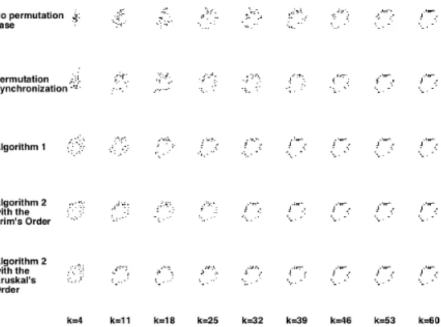
(a) The PCA reconstruction errors of our methods com-pared to two baseline methods. The horizontal axis rep-resents the reduction dimensionalityk. The performance of the two versions of Algorithm 2 are almost the same, and both clealy outperform previous approaches.

(b) The reconstructed results of an image of digit 0 by all methods. For each figure, we show the reconstructed images withk = 4,11,18, . . . ,60eigenvectors, respec-tively. We see that our methods can reconstruct the image well even atk = 4. Meanwhile, the other two methods require many more eigenvectors to reconstruct a recog-nizable digit 0 image.

Figure 2.1: Results for the PCA reconstruction experiment

2.4.1 PCA reconstruction of MNIST digits

Our first experiment is on image compression and recovery. We use theMNISTdataset [57], which contains 70,000 images of individual handwritten digits from{0, . . . ,9}.

In one experiment, we randomly selectedn = 100images I1, . . . ,Infrom the dataset, where each

digit has roughly₁₀n images. Note that we do not use a larger number of images because of scaleabil-ity limitations of [34] which we need as our baseline in the evaluation. Our algorithms, however, easily scale to much larger datasets. The goal of this experiment is to compress the MNIST im-ages with low dimensionality. We represent each imageIias an element set by randomly selecting

m = 30 _{white pixels (the MNIST digits are white drawings on a black background). This forms} the element set Xi = {xi_j = (ai_j,bi_j) : j ∈ {1, . . . ,m}}, where (aij,b

i

j) is the coordinate of the j t h

selected pixel of imageIi.

We will use Principal Components Analysis (PCA) as our compression technique and apply it to the element setsX1, . . . ,Xn. We can view each Xi as a matrixYi ∈ Rm×2where the jt h row ofYiis