Comparative Analysis of Predictive Models for the Likelihood of Infertility in Women Using Supervised Machine Learning Techniques
Jeremiah Ademola Balogun, Ngozi Chidozie Egejuru, and Peter Adebayo Idowu
Department of Computer Science and Engineering, Obafemi Awolowo University, Ile-Ife, Osun State, Nigeria [email protected]
Abstract
Infertility is a worldwide problem, affecting 8% – 15% of the couples in their reproductive age. WHO estimates that there are 60 - 80 million infertile couples worldwide with the highest incidence in some regions of Sub-Saharan Africa also infertility rate may reach 50% compared to 20% in Eastern Mediterranean Region and 11% in the developed world. Infertility has caused considerable social, emotional and psychological stress between couples, among families, within the individual concerned and the society at large. Historical data constituting information describing the risk factors of infertility alongside the respective infertility likelihood status of women was collected from Obafemi Awolowo University Teaching Hospital Complex (OAUTHC). The predictive model was formulated using naïve Bayes’, decision trees and multi-layer perceptron algorithm – supervised machine learning algorithms. The formulated model was simulated using the Waikato Environment for Knowledge Analysis (WEKA) environment. The results of the performance evaluation of the machine learning algorithms showed that the C4.5 decision trees and the multi-layer perceptron with an accuracy of 74.4% each outperformed the naïve Bayes’ algorithm. In addition, the decision trees algorithm recognized variables relevant to predicting infertility and a rule that can be applied on patient risk factor records for infertility likelihood prediction was deduced from the tree structure. This showed how effective machine learning algorithms can be used in predicting the likelihood of infertility in Nigerian women.
Keywords: prediction model, infertility in women, multi-layer perceptron, decision trees, naïve bayes. Introduction
While there is no universal definition of infertility, a couple is generally considered clinically infertile when pregnancy has not occurred after at least twelve months of regular sexual activity without the use of contraceptives [1]. Primary infertility is defined as childlessness and secondary infertility as the inability to have an additional live birth for a parous woman. Although women's infertility is of greater research consideration, health care attention and social blame, male conditions cause or contribute to around half of all cases of infertility [2]. According to World Health Organization, infertility is defined as one year of frequent, unprotected intercourse during which pregnancy has not occurred [3]. In another definition, infertility is the inability of a sexually active woman who is not practicing contraception to have a live birth [4].
Early exposures (e.g. in utero or in childhood) could permanently reprogram men and women for fecundity or biologic capacity (e.g. gynecologic and urologic health or gravid health during pregnancy) and fertility outcomes (e.g. multiple births or gestational age at delivery), which could affect later adult on set diseases [5]. Thus, infertility could have public health implications beyond simply the inability to have children. Infertility can be attributed to any abnormality in the female or male reproductive system [3]. The etiology is mostly distributed fairly equally among the male and female with factors ranging from ovarian dysfunction, tubal factors amongst others. A smaller percentage of cases are attributed to endometriosis, uterine or cervical factors, or other causes. In approximately, one fourth of couples, the cause is uncertain and is referred to as unexplained infertility, while etiology is multifactorial for some couples [6].
In general, an infertility evaluation is initiated after 12 months of unprotected intercourse during which pregnancy has not been achieved. Earlier investigation may be considered when historical factors, such as previous pelvic inflammatory disease or amenorrhea suggest infertility, although physicians should be aware
that earlier evaluation may lead to unnecessary testing and treatment in some cases. Evaluation also may be initiated earlier when the female partner is older than 35 years, because fertility rates decrease and spontaneous miscarriage and chromosomal abnormality rates increase with advancing maternal age [7]. Partners should be evaluated together and separately, because each person may want to reveal information about which their partner is unaware, such as previous pregnancy or sexually transmitted disease.
The risk factors for infertility can be classified into: genital, endocrinal, developmental and general factors. Pelvic inflame ematory disease (PID) due to sexually transmitted diseases, unsafe abortion, or puerperal infection is the main cause of tubal infertility caused mainly by chlamydial infection. Polycystic ovarian syndrome (PCOS) is thought to be the commonest cause of an ovulatory infertility [8]. Several lifestyle factors may affect reproduction, including habits of diet, clothing, exercise, and the use of alcohol, tobacco and recreational drugs. Exposure to textile dyes, lead, mercury and cadmium, volatile organic solvents and pesticides has been also associated with infertility [9]. Estimates of the proportion of infertility cases attributable to male or female specific factors in developed countries were derived in the 1980s by the WHO: 8% of infertility cases were attributable to male factors, 37 % to female factors, 35 % to both the male and female, and 5 % to an unknown cause (the remaining 15 % became pregnant) [10].
Prediction involves some variables or fields in the data set to predict unknown or future values of other variables of interest. On the other hand, description focuses on finding patterns describing the data that can be interpreted by humans. Machine learning plays an important role in disease prediction by identifying related pattern that exists between the risk factors associated with the likelihood of infertility in women. This will improve the level of decision-support offered to the expert gynecologist during the course of diagnosis. This study presents a comparative analysis between three (3) supervised machine learning model used to develop predictive models for the likelihood of infertility in women in order to propose the most effective and efficient model. Where possible, variables that are relevant to predicting the likelihood of infertility in women alongside their underlying relationship will also be proposed.
Related Works
There are different types of diseases whose likelihood or survival had been predicted using data mining technique namely Hepatitis and other liver disorders, Breast cancer, Thyroid disease, Diabetes, HIV/AIDS and Tuberculosis etc., for the purpose of this research, the prediction of likelihood of infertility in women, research work that are related to fertility were reviewed. There existed a number of research areas concerning infertility but none attempts to predict its likelihood in women using data mining technique, further to its prediction is the usage of a graphical user interface or rather a software system.
Durairaj and Kumar [11] worked on Selection of Influential Parameters on Fertility using a data mining method of data analysis, as classification is proposed for the In-Vitro Fertilization (IVF) data analysis, and multilayer perceptron network for classification or prediction. From the experiments, the observation was made in the attribute selection analysis and it helped to identify the most influential IVF parameters to predict the successful rate of IVF treatment. The proposed technique was useful for finding the minimum set of influential parameters in order to predict a success rate of IVF, which enabled the gynecologists to prescribe the treatment to the couples. By knowing the success rate prior to the treatment, the couples get psychological boost, which increases their chances of getting successful pregnancy.
Saith et al. [12] used decision trees to investigate the relationship of the features of the embryo, oocyte and follicle to the successful outcome of the embryo transfer. Although 53 features were studied, only 4 had predictive capabilities, embryo grade, cell number, follicle size and follicular fluid volume. This study used 200 IVF records and significantly differs from our study in that it did not consider any clinical data on the female and male patients involved in the procedure.
Shen et al [13]used statistical analysis to examine factors involved in IVF procedures. This study, however, only considered fertilizations accomplished with Intracytoplasmic Sperm Injection (ICSI). Statistical approaches were used to find that sperm motility and ICSI operator were the two most important predictors for the success of an IVF procedure. Sperm motility and ICSI technician were also features considered in the study. The data set was drastically different because the ICSI method of fertilization was used in only 44 % of their records.
Methods Data Collection
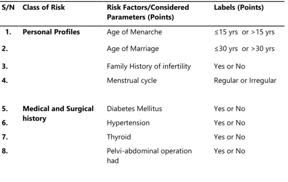
For the purpose of this study, it was necessary to identify and collect the data needed for identifying infertility in women from gynecologist located at the Obafemi Awolowo University Teaching Hospital Complex (OAUTHC) and the Faculty of Health Sciences of Obafemi Awolowo University, Ile-Ife. The variables identified include: age of menarche, age of marriage, family history of infertility, menstrual cycle, diabetes mellitus, hypertension, thyroid disease, pelvi-abdominal operation, endometriosis, fibroid disease, polycystic ovary, genital infection, previous termination of pregnancy, Sexually Transmitted Infection (STI) and the likelihood of infertility (identified using the labels: Likely, Unlikely and Probably) (Table 1). Data was collected from a total of 39 patients with a description of the variables in the dataset stated as follows:
a. Age of Menarche: is the identification of the age of the patient at first menstruation; it is recorded as a nominal value which determines the age category in years identified as equal or less than 15 years and greater than 15 years.
b. Age of marriage: is the identification of the patient’s age of marriage; it is recorded as a nominal value less than or equal to 30 years and greater than 30 years.
c. Menstrual cycle: is the identification of the regularity of the patient’s menstrual cycle; it is a nominal value identified as Regular or Irregular.
d. Family history of Infertility: is the identification of an existing history of infertility in the family; it is a nominal value identified as either Yes or No.
Table 1: Identified variables for determining infertility S/N Class of Risk Risk Factors/Considered
Parameters (Points)
Labels (Points) 1. Personal Profiles Age of Menarche ≤15 yrs or >15 yrs
2. Age of Marriage ≤30 yrs or >30 yrs
3. Family History of infertility Yes or No
4. Menstrual cycle Regular or Irregular
5. Medical and Surgical history
Diabetes Mellitus Yes or No
6. Hypertension Yes or No
7. Thyroid Yes or No
8. Pelvi-abdominal operation
had
9. Gynecological history Endometriosis No or Yes
10. Fibroid No or Yes
11. Polycystic Ovary No or Yes
12. Genital Infection No or Yes
13. Sexually transmitted Infection
(STI)
No or Yes
14. Previous termination of
pregnancy
No or Yes
e. Diabetes Mellitus: is the identification of the existence of diabetes disease in the patient; it is a nominal value identified as either Yes or No.
f. Hypertension: is the identification of if the patient has hypertension before or presently or not; it is a nominal value identified as either Yes or No.
g. Thyroid Disease: is the identification of the existence of thyroid disease in the patient; it is a nominal value identified as either Yes or No.
h. Pelvi-abdominal operation had: is the identification of the existence of pelvi-abdominal operation on the patient; it is a nominal value identified as either Yes or No.
i. Endometriosis: is the identification of the existence of Endometriosis in the patient; it is a nominal value identified as either Yes or No.
j. Fibroid disease: is the identification of the existence of fibroid disease in the patient; it is a nominal value identified as either Yes or No.
k. Polycystic ovary: is the identification of the patient having a polycystic ovary; it is a nominal value identified as either Yes or No.
l. Genital infection: is the identification of a genital infection in the patient; it is a nominal value identified as either Yes or No.
m. Previous termination of pregnancy: is the identification of the patient having a previous termination of pregnancy; it is a nominal value identified as either Yes or No.
Data-Preprocessing
Following the collection of data from the required respondents; 39 patients with their respective attributes (14 infertility risk indicators) alongside the likelihood of infertility was identified. In addition, the task of data cleaning for noise removal (errors, misspellings etc.) and missing data were performed on the information collected from the health records. Following this process, all data cells describing the attributes (fields) of each patient were found to be filled. No missing data were found in the repository and all misspellings were corrected.
In order for the dataset collected to be fit for the simulation environment; the dataset was converted to a more compactible data storage format. This would make the dataset fit for all the necessary machine learning operations performed by the simulation environment. Important to the study is the ability of the machine learning techniques to identify the most important combination of features that are more likely to improve the predicting the likelihood of infertility.
The dataset collected was converted to the required format needed for simulation; the Waikato Environment for Knowledge Analysis (WEKA) called the attribute relation file format (.arff) – a light-weight java application with a number of supervised and unsupervised machine learning tools. This format allows for the formal identification of the file name, attribute names and labels alongside the dataset that correspond to each attribute expressed using their respective labels. Figure 1 shows the format of the .arff file format chosen for the formal representation of the dataset using the 39 patient data collected.
Figure 1: arff file containing identified attributes Model Formulation
Systems that construct classifiers are one of the commonly used tools in data mining. Such systems take as input a collection of cases, each belonging to one of a small number of classes and described by its values for a fixed set of attributes, and output a classifier that can accurately predict the class to which a new case belongs. Supervised machine learning algorithms make it possible to assign a set of records (infertility risk indicators) to a target classes – the risk of infertility (Unlikely, Likely and Benign).
Supervised machine learning algorithms are Black-boxed models, thus it is not possible to give an exact description of the mathematical relationship existing among the independent variables (input variables) with respect to the target variable (output variable – risk of infertility). Cost functions are used by supervised machine learning algorithms to estimate the error in prediction during the training of data for model development. Gradient decent and other related algorithms are used to reduce the error by estimating cost function parameters.
Naïve Baye’s Classifier
Naive Bayes Classifier is a probabilistic model based on Baye’s theorem. It is defined as a statistical classifier. It is one of the frequently used methods for supervised learning. It provides an efficient way of handling any number of attributes or classes which is purely based on probabilistic theory. Bayesian classification provides practical learning algorithms and prior knowledge on observed data.
If X is a data sample containing instances, Xi where each instances are the infertility likelihood risk factors. Let H be a hypothesis that X belongs to class C which contains likely, probable and unlikely cases. Classification requires the determination of the following:
• P(Hj|X) – the posteriori probability: the probability that the hypothesis, Hj (unlikely, benign or likely) holds given the observed data sample X.
• P(Hj) - prior probability: the initial probability of the class, j;
• P(Xi): probability that sample data is observed for each attribute, i;
• P(Xi|H) - likelihood: the probability of observing the sample’s attribute, Xi given that the hypothesis holds in the training data X; and
The posteriori probability of a hypothesis Hj defined as either of unlikely, likely or benign, P(Hj|Xi), follows the Baye’s theorem as follows:
𝑃(𝐻𝑗|𝑋) =
∏𝑛𝑖=1𝑃(𝑋𝑖|𝐻𝑗)𝑃(𝑋𝑖)
𝑃(𝐻𝑗)
𝑓𝑜𝑟 𝑗 = 1,2,3 (1)
Where 𝑋 = {𝑋1, 𝑋2, 𝑋3… … . . 𝑋𝑛} is the set of risk factors for infertility likelihood of each patient, X and 𝐻𝑗= {𝐻1=
𝑙𝑖𝑘𝑒𝑙𝑦, 𝐻2= 𝑝𝑟𝑜𝑏𝑎𝑏𝑙𝑒, 𝐻3= 𝑢𝑛𝑙𝑖𝑘𝑒𝑙𝑦} is the target class set.
The breast cancer risk output class is thus:
𝑚𝑎𝑥. [𝑃(𝐻𝑗|𝑋)] 𝑓𝑜𝑟 𝑗 = 1, 2, 3. (2)
Decision Trees Algorithm
The theory of a decision tree has the following parts: a root node is the starting point of the tree; branches connect nodes showing the flow from question to answer. Nodes that have child nodes are called interior nodes. Leaf or terminal nodes are nodes that do not have child nodes and represent a possible value of target variable given the variables represented by the path from the root. The rules are inducted by definition from each respective node to branch to leaf.14
Splitting points attribute variables and values of chosen variables are chosen based on Gini impurity (eqn. 3) and Gini gain (eqn. 4) as expressed below by Chaurasia et al.14:
𝑖(𝑡) = 1 − ∑ 𝑓(𝑡, 𝑖)2= ∑ 𝑓(𝑡, 𝑖)𝑓(𝑡, 𝑗) 𝑖≠𝑗 𝑚 𝑖=1 (3) ∆𝑖(𝑠, 𝑡) = 𝑖(𝑡) − 𝑃𝐿∙ 𝑖(𝑡𝐿) − 𝑃𝑅∙ 𝑖(𝑡𝑅) (4)
Where 𝑓(𝑡, 𝑖) is the probability of getting i in node t, and the target variable takes values in {1, 2, 3… m}. 𝑃𝐿 is
the proportion of cases in node t divided to the left child node and 𝑃𝑅 is the proportion of cases in t sent to the
right child node. If the target variable is continuous, the split criterion is used with the Least Squares Deviation (LSD) as impurity measure. If there is no Gini gain or the preset stopping rule are satisfied, the splitting process stops.
Given a set S of cases, C4.5 first grows an initial tree using the divide-and-conquer algorithm as follows:
• If all the cases in S belong to the same class or S is small, the tree is a leaf labeled with the most frequent class in S.
• Otherwise, choose a test based on a single attribute with two or more outcomes. Make this test the root of the tree with one branch for each outcome of the test, partition S into corresponding subsetsS1, S2,...according to the outcome for each case, and apply the same procedure recursively to each subset.
ID3 (Iterative Dichotomiser 3) developed by Ross Quinlian15 is a classification tree used in the concept of information entropy. This provides a method to measure the number of bits each attribute can provide, and the attribute that yields the most information gain becomes the most important attribute and it should go at the top of the tree. Repeat this procedure until all the instances in the node are in the same category.
In this study, there are three outcomes, namely: Likely (u1), Unlikely (u2) and probably (u3) in the root node T of target variable. Let u1, u2 and u3 denote the number of probable, unlikely and likely records, respectively. The initial information entropy is given by equation 5 as:
𝐼(𝑢1, 𝑢2, 𝑢3) = − ∑ 𝑢𝑖 𝑢1+ 𝑢2+ 𝑢3 log2 𝑢𝑖 𝑢1+ 𝑢2+ 𝑢3 3 𝑖=1 (5)
If attribute X (a risk indicator of infertility) with values {x1 and x2} is chosen to be the split predictor and partition the initial node into {T1, T2, T3… TN}, and u1, u2 and u3 denote the number of probable, unlikely and likely records in the child node j. The expected information entropy, EI(X) and information gain, G(X) are given by:
𝐸𝐼(𝑋) = ∑𝑢1𝑗+ 𝑢2𝑗+ 𝑢3𝑗 𝑢1+ 𝑢2+ 𝑢3 ∙ 𝐼(𝑢1, 𝑢2, 𝑢3) 𝑁 𝑗=1 , (6) 𝐺(𝑋) = 𝐼(𝑢1, 𝑢2, 𝑢3) − 𝐸𝐼(𝑋) (7)
In 1993, Ross Quinlan made several improvements to ID.3 and extended it to C4.515. Unlike ID.3 which deals with discrete attributes, C4.5 handles both continuous and discrete attributes by creating a threshold to split the attribute into two groups, those above the threshold and those that are up to and including the threshold. C4.5 also deals with records that have unknown attribute values. C4.5 algorithm used normalized information gain or gain ratio as a modified splitting criterion of information gain which is the ratio of information gain divided by the information due to the split of a node on the basis of the value of a specific attribute. The reason of this modification is that the information gain tends to favor attributes that have a large number of values.
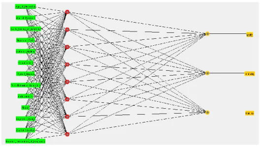
Multi-layer Perceptron Architecture
Multi-layer perception (MLP) is a natural extension of the single layer perception network of the class of artificial neural networks used in artificial intelligence. It is characterized by a forward flow of a set of inputs passing through subsequent hidden and computational layers composed by perception neurons using the feed-forward algorithm (Figure 3). The usage of MLPs is defended by the fact that they are able to predict and detect more complicated patterns in data. This is because multi-layer perceptron uses an additional algorithm which is called the back-propagation algorithm.
Figure 3: Structure of the multi-layer perceptron architecture The back-propagation algorithm used in this study to train the network consists of two steps:
i.Step 1 - Forward pass: the inputs are passed through the network layer by layer and an output is produced. During this step, the synaptic weights are fixed; and
ii.Step 2 - Backward pass: the output from step 1 is compared to the target producing an error signal. That is propagated backwards. The aim of this step is to reduce the error in a statistical sense by adjusting the synaptic weights according to a defined scheme.
The multilayer perception has the following characteristics:
i.At all neurons within the network feature, a nonlinear activation function that is differentiable is present everywhere;
ii.The network has one or more hidden layers made up of neurons that are removed from direct contact with input and output. These neurons calculate a signal expressed as a nonlinear function of its input with synaptic weights and an estimate of the gradient vector; and
iii.There is a high degree of interconnectivity within the network.
The mathematical model of the multi-layer perceptron in Figure 3 is as follows:
• The Input Layer
In this part of the multi-layer perception (MLP) the input values, Xn (factors responsible for infertility in women) are entered into the MLP system where n is the number of attributes (n=14 in this study) and the weights, Wi of each input, Xi produce a summation, Uk which is added to a bias variable, X0 (takes a value of 0 or 1) all equal to Vk is sent to the hidden layer for the activation function, φ to take effect where k is the hidden layer. The Summation Uk has the expression as follows:
𝑈𝑘 = 𝑤1𝑥1 + 𝑤2𝑥2 + 𝑤3𝑥3 + 𝑤4𝑥4 + ⋯ + 𝑤𝑛𝑥𝑛 (8𝑎)
𝑇ℎ𝑢𝑠, 𝑉𝑘= 𝑈𝑘 + 𝑥0 (8𝑏)
Where 𝑋𝑛= {𝑥1, 𝑥2, 𝑥3, ⋯ , 𝑥𝑛} is the patient’s record containing the factors considered predictive for the
And n = 14 attributes (input variables, xn)
• The Hidden Layer
At this part of the MLP the summation of the input variables are all sent to the activation function which is fired through all the hidden layers (for the purpose of this study 20 layers was used) using the activation function called the sigmoid function. The sigmoid function is expressed as:
𝑆𝑖𝑔𝑚𝑜𝑖𝑑 𝑓𝑢𝑛𝑐𝑡𝑖𝑜𝑛, 𝜑 = 1
1 + 𝑒−𝑎𝑣 (9)
Where 𝑎𝜖ℝ is a shape parameter of the sigmoid function And 𝑣 = 𝑉𝑘
• The Output Layer
At this point, the value of the output (infertility status) is determined with the error rate as low as possible. Also, the back-propagation algorithm is applied which tries to reduce the error rate, of the model via gradient descent by adjusting the values of the synaptic weights before the neuron fires the next set of inputs. At iteration m (the mth row in the training set) which in this case is 39, the error for neurons in the output layer is calculated in order to determine the error in computation. The error is calculated thus:
𝑒𝑟𝑟𝑜𝑟, 𝜀 = 𝑦𝑝𝑖− 𝑦𝑎𝑖 (10) 𝑔𝑟𝑎𝑑𝑖𝑒𝑛𝑡 𝑑𝑒𝑠𝑐𝑒𝑛𝑡 𝑖𝑠 lim 𝑡=𝑘 𝑑𝜀 𝑑𝑡= 0 𝑤ℎ𝑒𝑟𝑒 𝑡 = 𝑘 𝑖𝑠 𝑡ℎ𝑒 𝑛𝑢𝑚𝑏𝑒𝑟 𝑜𝑓 𝑖𝑡𝑒𝑟𝑎𝑡𝑖𝑜𝑛𝑠 𝑚𝑒𝑎𝑛 𝑠𝑞𝑢𝑎𝑟𝑒 𝑒𝑟𝑟𝑜𝑟 = 1 2𝑚 ∙ ∑ (𝑦𝑝𝑖− 𝑦𝑎𝑖) 2 𝑚 𝑖=1 (11) Where ypi and yai are the predicted and actual output for patient, i
And m is the total patient data (m = 39) Performance Evaluation
Following the development of the predictive model using all the proposed methods, the performance of the model was evaluated using the confusion matrix to determine the value of the performance metric chosen for this study. A confusion matrix contains information about actual and predicted classification done by a classification system and its performance is commonly evaluated using the data in the matrix (Figure 4). In this study, the likely cases are the positive cases while the probable and unlikely cases are the negative cases. Also, correctly classified cases are placed in the true cells (positive and negative) while incorrect classifications are placed in the false cells (positive and negative) and this has generated the rule (i) to (iv), below:
i.True positives (TP) are correctly classified positive cases; ii.False positives (FP) are incorrectly classified positive cases; iii.True negatives (TN) are correctly classified negative cases; and iv.False negatives (FN) are incorrectly classified negative cases.
Figure 4: Diagram of a Confusion Matrix
From a confusion matrix, different measures of the performance of a prediction model can be determined using the values of the true positive/negatives and false positives/negatives. For the purpose of this study, the positive cases are the Likely Cases of infertility while the negative cases are probably and Unlikely cases.
a. True Positive rates (TP rates/Recall) – proportion of positive cases correctly classified
𝑇𝑃 𝑟𝑎𝑡𝑒 = 𝑇𝑃
𝑇𝑃 + 𝐹𝑁 (12)
b. False Positive rates (FP rates/False alarms) – proportion of negative cases incorrectly classified as positives
𝐹𝑃 𝑟𝑎𝑡𝑒 = 𝐹𝑃
𝐹𝑃 + 𝑇𝑁 (13) c. Precision – proportion of predicted positive cases that were correct
𝑃𝑟𝑒𝑐𝑖𝑠𝑖𝑜𝑛 = 𝑇𝑃
𝑇𝑃 + 𝐹𝑃 (14) d. Accuracy – proportion of the total predictions that was correct.
𝐴𝑐𝑐𝑢𝑟𝑎𝑐𝑦 = 𝑇𝑃 + 𝑇𝑁
𝑇𝑃 + 𝑇𝑁 + 𝐹𝑃 + 𝐹𝑁 (15) Results
Data Description
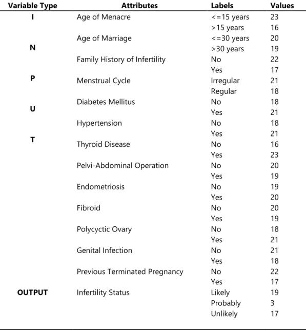
The data containing information about the attributes and the respective infertility status for 39 patients is shown in Table 2 alongside the distribution of the data shown in Figure 5. It was observed that out of the 39 patients, 19 were likely infertile, 3 were probably infertile and 17 were unlikely infertile. The highest distribution was: 23 with age of menacre less than or equal to 15 years, 23 had thyroid disease, 22 had no family history of infertility, 20 had no previous terminated pregnancy, 21 had irregular menstrual cycle, 21 had diabetes mellitus, 21 had hypertension, 21 had polycyctic ovary and 21 had no genital infection.
The lowest distribution was: 16 had age of menacre more than 15 years, 16 had no thyroid disease, 17 had family history of infertility, 17 had previously terminated pregnancy, 18 had irregular menstrual cycle, 18 had no diabetes mellitus, 18 had no hypertension, 18 had no polycyctic ovary and 18 had genital infection.
Table 2: Description of the identified variables
Variable Type Attributes Labels Values
I
N
P
U
T
Age of Menacre <=15 years 23
>15 years 16
Age of Marriage <=30 years 20
>30 years 19 Family History of Infertility No 22
Yes 17
Menstrual Cycle Irregular 21
Regular 18 Diabetes Mellitus No 18 Yes 21 Hypertension No 18 Yes 21 Thyroid Disease No 16 Yes 23 Pelvi-Abdominal Operation No 20 Yes 19 Endometriosis No 19 Yes 20 Fibroid No 20 Yes 19 Polycyctic Ovary No 18 Yes 21 Genital Infection No 21 Yes 18
Previous Terminated Pregnancy No 22
Yes 17
OUTPUT Infertility Status Likely 19
Probably 3 Unlikely 17
Simulation Results
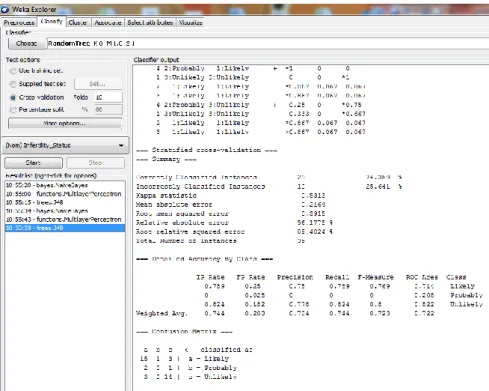
Three different supervised machine learning algorithms were used to formulate the predictive model for the likelihood of infertility; they were used to train the development of the prediction model using the dataset containing 39 patients’ risk factor records. The simulation of the prediction models was done using the Waikato Environment for Knowledge Analysis (WEKA). The C4.5 decision trees algorithm was implemented using the J48 decision trees algorithm available in the trees class, the naïve Bayes’ algorithm was implemented using the naïve Bayes’ classifier available in the Bayes class while the Multi-layer perceptron was implemented using the multi-layer perceptron classifier available in the functions class all available on the WEKA environment of classification tools. The models were trained using the 10-fold cross validation method which splits the dataset into 10 subsets of data – while 9 parts are used for training the remaining one is used for testing; this process is repeated until the remaining 9 parts take their turn for testing the model.
Results of the naïve Bayes’ classifier
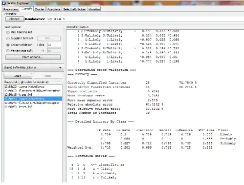
Using the naïve Bayes’ classifier to train the predictive model developed using the training data via the 10-fold cross validation method, it was discovered that there were 28 (71.79%) correct classifications and 11 (28.21%) incorrect classifications – showing an accuracy of 71.8% (Figure 5).
Figure 5: Simulation results for naïve Bayes’ classifier
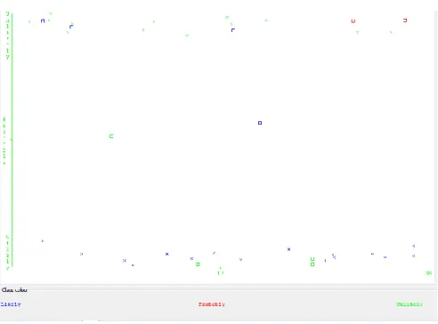
Using the confusion matrix, it was discovered that out of 19 likely cases there were 15 correct classifications while1 misclassified for probable and 3 for unlikely. Out of 3 probable cases there were no correct classifications while 1 misclassified for likely and 2 for unlikely. Out of 17 unlikely cases there were 13 correct classifications with 3 misclassified for likely and 1 for probable (Figure 6 – left). Figure 7 shows a graphical plot of the correct and incorrect classifications – correct classifications are crosses while incorrect classifications are boxes.
Figure 7: Graphical plot of simulation results for naïve Bayes’ Results of the C4.5 decision trees classifier
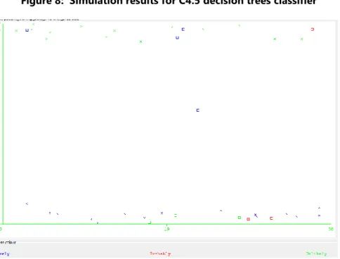
Using the C4.5 decision trees classifier to train the predictive model developed using the training data via the 10-fold cross validation method, it was discovered that there were 29 (74.36%) correct classifications and 10 (25.64%) incorrect classifications – showing an accuracy of 74.4% (Figure 8). Using the confusion matrix, it was discovered that out of 19 likely cases there were 15 correct classifications while1 misclassified for probable and 3 for unlikely. Out of 3 probable cases there were no correct classifications while 2 misclassified for likely and 1 for unlikely. Out of 17 unlikely cases there were 14 correct classifications with 3 misclassified for likely (Figure 6 – middle). Figure 9 shows a graphical plot of the correct and incorrect classifications – correct classifications are crosses while incorrect classifications are boxes.
Figure 8: Simulation results for C4.5 decision trees classifier
Figure 9: Graphical plot of simulation results for C4.5 decision trees
For every decision trees algorithm there is always a hierarchical tree with an attributes at each node form the parent node all the way to the child node to the leave - the target class. The tree can be coverted to a rule by following the patten from the parent ode at the top all the way to the child node until the bottom leaf is achieved where the necessary classification is defined. Figure 10 shows the decision trees constructed during the model development; it can be seen that a number of variables were identified as been relevant for infertility likelihood prediction. It can also be discovered that the size of the tree is 6 and the number of leaves plotted are 5. The variables identified are:
• Prevous termination of pregnancy
• Menstrual Cycle
• Age of Manacre and
Figure 10: Graphical plot of the decision tree for infrtility likelihood
Using the decision tree in Figure 10, the following rule can be used to predict the likelihood of infertility in women given the values of the four identified risk factors. The rule can be read as follows:
IF Previous Termination of Pregnancy = “Yes” THEN infertility likelihood = “Likely” Else IF Previous Termination of Pregnancy = “No” THEN
IF Menstrual Cycle = “Regular” THEN infertility likelihood = “Unlikely” Else IF Menstrual Cycle = “Irregular” THEN
IF Age of Menacre = “>15 years” THEN infertility likelihood = “Probable” Else If Age of Menacre = “<=15 years” THEN
IF Genital Infection = “Yes” THEN infertility likelihood = “Likely” Else IF Genital Infection = “No” THEN infertility likelihood = “Unlikely”
Results of the Multi-Layer Perceptron (MLP) classifier
Using the Multi-layer perceptron classifier to train the predictive model developed using the training data via the 10-fold cross validation method, it was discovered that there were 29 (74.36%) correct classifications and 10 (25.64%) incorrect classifications – showing an accuracy of 74.4% (Figure 11). Using the confusion matrix, it was discovered that out of 19 likely cases there were 16 correct classifications while 2 misclassified for probable and 1 for unlikely. Out of 3 probable cases there were no correct classifications while 1 misclassified for likely and 2 for unlikely. Out of 17 unlikely cases there were 13 correct classifications with 1 misclassified for likely and 3 for probable (Figure 6 – right). Figure 12 shows a graphical plot of the correct and incorrect classifications – correct classifications are crosses while incorrect classifications are boxes.
Figure 11: Simulation results for C4.5 decision trees classifier
Figure 12: Graphical plot of simulation results for C4.5 decision trees Discussions
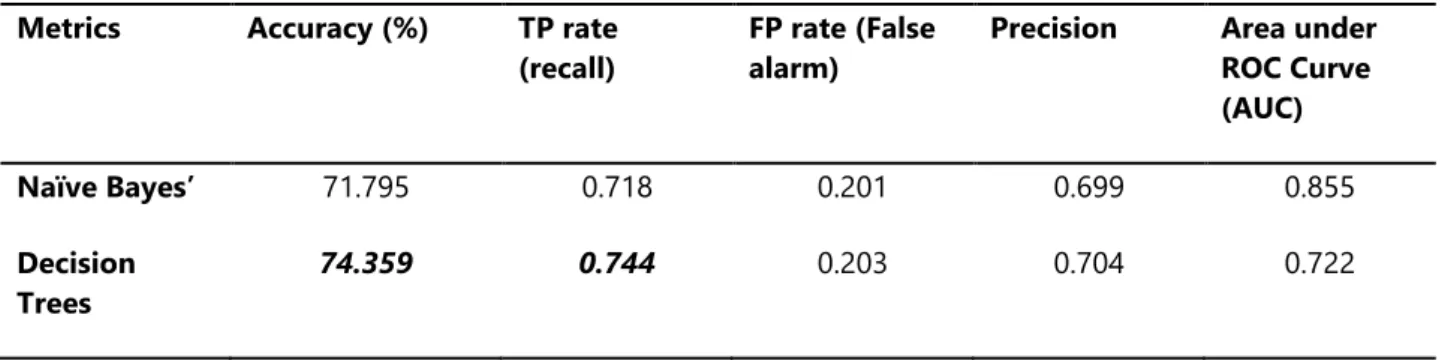
Table 3 gives a summary of the simulation results by presenting the average value of each performance metrics that was evaluated for the machine learning techniques used. The True positive rate (recall/sensitivity), false positive rate (false alarm/1-specificity), precision, accuracy and the area under the receiver operating characteristics (ROC) curve were used. From the table, it was discovered that the decision trees and the MLP algorithms showed the highest accuracy due to the ability to predict 29 out of the 39 records correctly. The true positive rate was also highest for the decision trees and the MLP algorithms with an equal value of 0.744 – which implies that 74.4% of the actual positive cases (likely) were correctly classified. The MLP showed the lowest value for the false positive rate with a value of 0.119 – which implies that 11.9% of the actual negative classes (probable or unlikely) were misclassified for positive cases. The MLP also had the highest value for the precision with a value of 0.787 – which implies that 78.7% of the positive classifications made were actually positive classes. The decision trees algorithm was observed to have the lowest area under the receiver operating characteristics (ROC) curve – a graph of the TP rate against the FP rate which had a value of 0.722. The area under the graph is used to identify the level of relevance that can be given to the machine learning algorithm at making predictions – thus, the higher the value then the lower the bias of the model.
Table 3: Summary of simulation results
Metrics Accuracy (%) TP rate
(recall)
FP rate (False alarm)
Precision Area under ROC Curve (AUC) Naïve Bayes’ 71.795 0.718 0.201 0.699 0.855 Decision Trees 74.359 0.744 0.203 0.704 0.722
Multi-layer Perceptron
74.359 0.744 0.119 0.787 0.862
From the simulation results, it can be inferred that the most effective supervised machine learning algorithm is the multi-layer perceptron (MLP) due to its high accuracy, TP rate and Precision with lower value for the FP rate. The variables identified and the rule deduced from the variables using the decision trees algorithm can also be used to support decision made by gynecologist concerning infertility likelihood in women.
Conclusions
In this paper, the development of a predictive model for determining the likelihood of infertility in Nigerian women was proposed using dataset collected from patients in Obafemi Awolowo University Teaching Hospital Complex (OAUTHC), Ile-Ife, Osun State in Nigeria. 14 variables were identified by gynecologist to be necessary in predicting infertility in women for which a dataset containing information of 39 patients alongside their respective infertility status (likely, unlikely and probably) was also provided with 14 attributes following the identification of the required variables.
After the process of data collection and pre-processing, three supervised machine learning algorithms were used to develop the predictive model for the likelihood of infertility in women using the historical dataset from which the training and testing dataset was collected. The 10-fold cross validation method was used to train the predictive model developed using the machine learning algorithms and the performance of the models evaluated.
The multi-layer perceptron proved to be an effective algorithm for predicting infertility in women given the attributes identified but it is believed that higher accuracy could be attained by increasing the number of records used and be identifying other relevant attributes which could help predict infertility in women. Rule induced algorithms can also be used to plot the relationship between the selected attributes identified with respect to determining the likelihood of infertility in women using the decision trees algorithm.
References