Deep Filter Banks for Texture Recognition, Description, and Segmentation

DOI 10.1007/s11263-015-0872-3

Deep Filter Banks for Texture Recognition, Description,

and Segmentation

Mircea Cimpoi1 · Subhransu Maji2 · Iasonas Kokkinos3 · Andrea Vedaldi1

Received: 4 June 2015 / Accepted: 20 November 2015 / Published online: 9 January 2016 © The Author(s) 2015. This article is published with open access at Springerlink.com Abstract Visual textures have played a key role in image

understanding because they convey important semantics of images, and because texture representations that pool local image descriptors in an orderless manner have had a tremendous impact in diverse applications. In this paper we make several contributions to texture understanding. First, instead of focusing on texture instance and material category recognition, we propose a human-interpretable vocabulary of texture attributes to describe common texture patterns,

complemented by a new describable texture dataset for

benchmarking. Second, we look at the problem of recog-nizing materials and texture attributes in realistic imaging conditions, including when textures appear in clutter, devel-oping corresponding benchmarks on top of the recently proposed OpenSurfaces dataset. Third, we revisit classic tex-ture represenations, including bag-of-visual-words and the Fisher vectors, in the context of deep learning and show that these have excellent efficiency and generalization prop-erties if the convolutional layers of a deep model are used as

Communicated by Svetlana Lazebnik.

B

1 _{University of Oxford, Oxford, UK}

2 _{University of Massachusetts Amherst, Amherst, USA} 3 _{CentraleSupélec/INRIA-Saclay, Palaiseau, France}

filter banks. We obtain in this manner state-of-the-art perfor-mance in numerous datasets well beyond textures, an efficient method to apply deep features to image regions, as well as benefit in transferring features from one domain to another. Keywords Texture and material recognition ·Visual

attributes·Convolutional neural networks·Filter banks·

Fisher vectors·Datasets and benchmarks

1 Introduction

Visual representations based on orderless aggregations of local features, which were originally developed as texture descriptors, have had a widespread influence in image under-standing. These models include cornerstones such as the

histograms of vector quantized filter responses ofLeung and

Malik(1996) and later generalizations such as the

bag-of-visual-words model ofCsurka et al.(2004) and the Fisher

vector of Perronnin and Dance (2007). These and other

texture models have been successfully applied to a huge variety of visual domains, including problems closer to “tex-ture understanding” such as material recognition, as well as domains such as object categorization and face identification that share little of the appearance of textures.

This paper makes three contributions to texture

under-standing. The first one is to add a newsemantic dimension

to the problem. We depart from most of the previous works on visual textures, which focused on texture identification and material recognition, and look instead at the problem of describing generic texture patterns. We do so by developing

a vocabulary of forty-seven texture attributesthat describe

a wide range of texture patterns; we also introduce a large dataset annotated with these attributes which we call the describable texture dataset(Sect.2). We then study whether

texture attributes can be reliably estimated from images, and for what tasks are they useful. We demonstrate in particular

two applications (Sect.8.1): the first one is to use texture

attributes as dimensions to organise large collections of tex-ture patterns, such as textile, wallpapers, and construction materials for search and retrieval. The second one is to use texture attributes as a compact basis of visual descriptors applicable to other tasks such as material recognition.

The second contribution of the paper is to introduce new data and benchmarksto study texture recognition in real-istic settings. While most of the earlier work on texture recognition was carried out in carefully controlled condi-tions, more recent benchmarks such as the Flickr material

dataset (FMD) (Sharan et al. 2009) have emphasized the

importance of testing algorithms “in the wild”, for example on Internet images. However, even these datasets are some-what removed from practical applications as they assume that textures fill the field of view, whereas in applications they are often observed in clutter. Here we leverage the

excel-lent OpenSurfaces dataset (Bell et al.(2013)) to create novel

benchmarks for materials and texture attributes where

tex-tures appear both in the wild and in clutter (Sect.3), and

demonstrate promising recognition results in these

challeng-ing conditions. InBell et al.(2015) the same authors have

also investigated material recognition using OpenSurfaces. The third contribution is technical and revisits classi-cal ideas in texture modeling in the light of modern loclassi-cal feature descriptors and pooling encoders. While texture rep-resentations were extensively used in most areas of image

understanding, since the breakthrough work ofKrizhevsky

et al.(2012) they have been replaced by deep Convolutional Neural Networks (CNNs). Often CNNs are applied to a prob-lem by using transfer learning, in the sense that the network is first trained on a large-scale image classification task such

as the ImageNet ILSVRC challenge (Deng et al.(2009)), and

then applied to another domain by exposing the output of a so-called “fully connected layer” as a general-purpose image representation. In this work we illustrate the many benefits of truncating these CNNs earlier, at the level of the

convolu-tional layers (Sect.4). In this manner, one obtains powerful

local image descriptorsthat, combined with traditional pool-ing encoders developed for texture representations, result in state-of-the-art recognition accuracy in a diverse set of visual domains, from material and texture attribute recognition, to coarse and fine grained object categorization and scene clas-sification. We show that a benefit of this approach is that features transfer easily across domains even without fine-tuning the CNN on the target problem. Furthermore, pooling allows us to efficiently evaluate descriptors in image subre-gions, a fact that we exploit to recognize local image regions without recomputing CNN features from scratch.

A symmetric approach, using SIFT as local features and the IFV followed by fully-connected layers from a deep

neural network as a pooling mechanism, was proposed in Perronnin and Larlus (2015), obtaining similar results on VOC07.

This paper is the archival version of two previous

pub-lications Cimpoi et al. (2014) and Cimpoi et al. (2015).

Compared to these two papers, this new version adds a sig-nificant number of new experiments and a substantial amount of new discussion.

The code and data for this paper are available on the project

page, athttp://www.robots.ox.ac.uk/~vgg/research/deeptex.

2 Describing Textures with Attributes

This section looks at the problem of automatically describ-ing texture patterns usdescrib-ing a general-purpose vocabulary of human-interpretable texture attributes, in a manner similar to

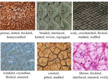
how we can vividly characterize the textures shown in Fig.1.

The goal is to design algorithms capable of generating and

understanding texture descriptions involving acombination

of describable attributesfor each texture. Visual attributes

have been extensively used insearch, to understand complex

user queries, inlearning, to port textual information back

to the visual domain, and in imagedescription, to produce

richer accounts of the content of images. Textural proper-ties are an important component of the semantics of images, particularly for objects that are best characterized by a

pat-tern, such as a scarf or the wings of a butterfly (Wang et al.

2009). Nevertheless, the attributes of visual textures have

been investigated only tangentially so far. Our aim is to fill this gap.

Our first contribution is to introduce the describable

textures dataset(DTD) (Cimpoi et al. 2014), a collection

Fig. 1 We address the problem ofdescribing texturesby associating to them a collection of attributes. Our goal is to understand and generate automatically human-interpretable descriptions such as the examples above

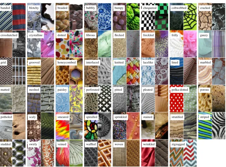
Fig. 2 The 47 texture words in thedescribable texture datasetintroduced in this paper. Two examples of each attribute are shown to illustrate the significant amount of variability in the data

of real-world texture images annotated with one or more adjectives selected in a vocabulary of forty-seven English

words. These adjectives, ordescribable texture attributes, are

illustrated in Fig.2and include words such asbanded,

cob-webbed,freckled,knitted, andzigzagged. Sect.2.1describes

this data in more detail. Sect.2.2discusses the technical

chal-lenges we addressed while designing and collecting DTD, including how the forty-seven texture attributes were selected and how the problem of collecting numerous attributes for

a vast number of images was addressed. Sect.2.3defines a

number of benchmark tasks in DTD. Finally, Sect.2.5relates

DTD to existing texture datasets.

2.1 The Describable Texture Dataset

DTD investigates the problem oftexture description,

under-stood as the recognition of describable texture attributes. This problem is complementary to standard texture analysis tasks such as texture identification and material recognition for the following reasons. While describable attributes are correlated

with materials, attributes do not imply materials (e.g.veined

may equally apply to leaves or marble) and materials do not

imply attributes (not all marbles areveined). This distinction

is further elaborated in Sect.2.4.

Describable attributes can be combined to create rich

descriptions (Fig. 3; marble can be veined, stratified and

cracked at the same time), whereas a typical assumption is that textures are made of a single material. Describable

attributes aresubjectiveproperties that depend on the imaged

object as well as on human judgements, whereas materials are objective. In short, attributes capture properties of tex-tures complementary to materials, supporting human-centric tasks where describing textures is important. At the same time, we will show that texture attributes are also helpful in

material recognition (Sect.8.1).

DTD contains textures in the wild,i.e. texture images

extracted from the web rather than captured or generated in a controlled setting. Textures fill the entire image in order to allow studying the problem of texture description indepen-dently of texture segmentation, which is instead addressed in

0 0.05 0.1 0.15

Occurrences per image

bandedblotchybraidedbubblybumpy chequeredcobwebbed

cracked crosshatched

crystalline dottedfibrousfleckedfreckled

frilly gauzygrid

grooved honeycombed

interlaced

knittedlacelikelinedmarbledmattedmeshedpaisley perforated pitted pleated polka−dotted porous potholed scaly

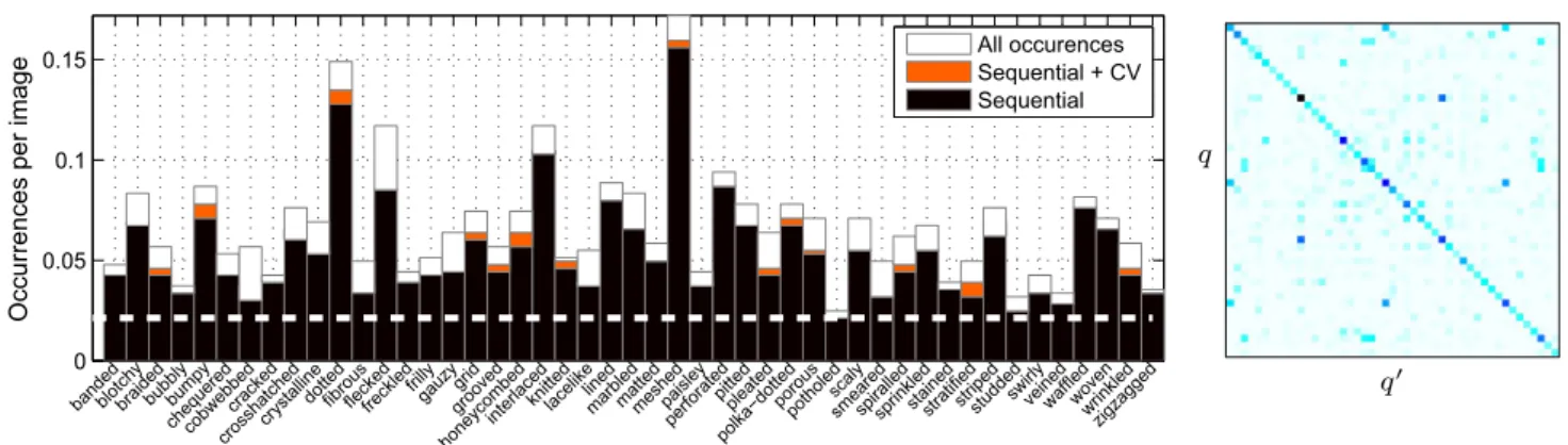
smearedspiralledsprinkledstainedstratifiedstripedstuddedswirlyveinedwaffledwovenwrinkled zigzagged All occurences Sequential + CV Sequential q q

Fig. 3 Quality of sequential joint annotations. Eachbar shows the average number of occurrences of a given attribute in a DTD image. Thehorizontal dashed line corresponds to a frequency of 1/47, the minimum given the design of DTD (Sect.2.2). Theblack portionof each bar is the amount of attributes discovered by the sequential pro-cedure, using only ten annotations per image (about one fifth of the

effort required for exhaustive annotation). Theorange portionshows the additional recall obtained by integrating cross-validation in the process. Right: co-occurrence of attributes.Thematrixshows the joint proba-bilityp(q,q)of two attributes occurring together (rows and columns are sorted in the same way as theleftimage) (Color figure online)

Sect.3. With 5640 annotated texture images, this dataset aims

at supporting real-world applications were the recognition of texture properties is a key component. Collecting images from the Internet is a common approach in categorization and object recognition, and was adopted in material recogni-tion in FMD. This choice trades-off the systematic sampling of illumination and viewpoint variations existing in datasets such as CUReT, KTH-TIPS, Outex, and Drexel to capture real-world variations, reducing the gap with applications. Furthermore, DTD captures empirically human judgements regarding the invariance of describable texture attributes; this invariance is not necessarily reflected in material properties.

2.2 Dataset Design and Collection

This section discusses how DTD was designed and collected, including: selecting the 47 attributes, finding at least 120 representative images for each attribute, and collecting all the attribute labels for each image in the dataset.

2.2.1 Selecting the Describable Attributes

Psychological experiments suggest that, while there are a few hundred words that people commonly use to describe textures, this vocabulary is redundant and can be reduced to a much smaller number of representative words. Our

starting point is the list of 98 words identified byBhushan

et al.(1997). Their seminal work aimed to achieve for tex-ture recognition the same that color words have achieved

for describing color spaces (Berlin and Kay 1991).

How-ever, their work mainly focuses on the cognitive aspects of texture perception, including perceptual similarity and the identification of directions of perceptual texture

variabil-ity. Since our interest is in the visual aspects of texture, words such as “corrugated” that are more related to surface shape or haptic properties were ignored. Other words such as “messy” that are highly subjective and do not necessarily correspond to well defined visual features were also ignored. After this screening phase we analyzed the remaining words and merged similar ones such as “coiled”, “spiraled” and “corkscrewed” into a single term. This resulted in a set of 47

words, illustrated in Fig.2.

2.2.2 Bootstrapping the Key Images

Given the 47 attributes, the next step consisted in collecting a sufficient number (120) of example images representative of each attribute. Initially, a large initial pool of about a hundred-thousand images in total was downloaded from Google and Flickr by entering the attributes and related terms as search queries. Then Amazon Mechanical Turk (AMT) was used to remove low resolution, poor quality, watermarked images, or images that were not almost entirely filled with a texture. Next, detailed annotation instructions were created for each of the 47 attributes, including a dictionary definition of each concept and examples of textures that did and did not match the concept. Votes from three AMT annotators were collected for the candidate images of each attribute and a shortlist of about 200 highly-voted images was further manually checked by the authors to eliminate remaining errors. The result was a

selection of 120key representative imagesfor each attribute.

2.2.3 Sequential Joint Annotation

So far only the key attribute of each image is known while any of the remaining 46 attributes may apply as well.

Exhaustively collecting annotations for 46 attributes and 5640 texture images is fairly expensive. To reduce this cost we propose to exploit the correlation and sparsity of the

attribute occurrences (Fig.3). For each attributeq, twelve

key images are annotated exhaustively and used to

esti-mate the probabilityp(q|q)thatanotherattributeq could

co-exist with q. Then for the remaining key images of

attributeq, only annotations for attributesqwith non

negli-gible probability are collected, assuming that the remaining attributes would not apply. In practice, this requires anno-tating around 10 attributes per texture instance, instead of 47. This procedure occasionally misses attribute annotations;

Fig.3evaluates attribute recall by 12-fold cross-validation on

the 12 exhaustive annotations for a fixed budget of collecting 10 annotations per image.

A further refinement is to suggest which attributes q

to annotate not just based on the prior p(q|q), but also

based on the appearance of an image xi. This was done

by using the attribute classifier learned in Sect. 6; after

Platt’s calibration (Platt 2000) on a held-out test set, the

classifier score cq(xi) ∈ R is transformed in a

probabil-ity p(q|xi)=σ(cq(x))whereσ (z)=1/(1+e−z)is the

sigmoid function. By construction, Platt’s calibration reflects

the prior probabilityp(q)≈p0=1/47 ofqon the

valida-tion set. To reflect the probabilityp(q|q)instead, the score

is adjusted as p(q|i,q)∝σ (cq(i))× p(q|q) 1−p(q|q)× 1−p0 p0

and used to find which attributes should be annotated for each

image. As shown in Fig.3, for a fixed annotation budget this

method increases attribute recall.

Overall, with roughly 10 annotations per image it was possible to recover all of the attributes for at least 75 % of the images, and miss one out of four (on average) for another 20 %, while keeping the annotation cost to a reasonable level. To put this in perspective, directly annotating the 5640 images for 46 attributes and collecting five annotations per attributed would have required 1.2M binary annotations, i.e. roughly 12K USD at the very low rate of 1¢ per annotation. Using the proposed method, the cost would have been 546 USD. In practice, we spent around 2.5K USD in order to pay annota-tors better as well as to account for occasional errors in setting up experiments and the fact that, as explained above, boot-strapping still relies on exhaustive annotations for a subset of the data.

2.3 Benchmark Tasks

DTD is designed as a public benchmark. The data, including images, annotations, and splits, is available on the web at

http://www.robots.ox.ac.uk/~vgg/data/dtd, along with code

for evaluation and reproducing the results in Sect.6.

DTD defines two challenges. The first one, denoted DTD,

is the prediction of key attributes, where each image is

assigned a single label corresponding to the key attribute defined above. The second one, denoted DTD-J, is the joint prediction of multiple attributes. In this case each image is assigned one or more labels, corresponding to all the attributes that apply to that image.

The first task is evaluated both in term of classifica-tion accuracy (acc) and in term of mean average precision (mAP), while the second task only in term of mAP due to the possibility of multiple labels. The classification

accu-racy is normalized per class: ifcˆ(x),c(x)∈ {1, . . . ,C}are

respectively the predicted and ground-truth label of imagex,

accuracy is defined as acc(cˆ)= 1 C C ¯ c=1 |{x:c(x)= ¯c∧ ˆc(x)= ¯c}| |{x:c(x)= ¯c}| . (1) We define mAP as per the PASCAL VOC 2008 benchmark

onwardEveringham et al.(2008).1

DTD contains 10 preset splits into equally-sized training, validation and test subsets for easier algorithm comparison. Results on any of the tasks are repeated for each split and average accuracies are reported.

2.4 Attributes Versus Materials

As noted at the beginning of Sect.2.1and inSharan et al.

(2013), texture attributes and materials are correlated, but

not equivalent. In this section we verify this quantitatively

on the FMD data (Sharan et al. 2009). Specifically, we

man-ually collected annotations for the 47 DTD attributes for the 1,000 images in the FMD dataset, which span ten different materials. Each of the 47 attributes was considered in turn,

using a categorical random variable C ∈ {1,2, . . . ,10}to

denote the texture material and a binary variable A∈ {0,1}

to indicate whether the attribute applies to the texture or not. On average, the relative reduction in the entropy of the

mate-rial variable I(A,C)/H(C)given the attribute is of about

14 %; vice-versa, the relative reduction in the entropy of the

attribute variable I(A,C)/H(A)given the material is just

0.5 %. We conclude that knowing the material or attribute

of a texture provides little information on the attribute or

material, respectively. Note thatcombinations of attributes

can predict materials much more reliably, although this is difficult to quantify from a small dataset.

2.5 Related Work

This section relates DTD to the literature in texture under-standing. Textures, due to their ubiquitousness and com-plementarity to other visual properties such as shape, have

been studied in several contexts: texture perception (

Adel-son 2001;Amadasun and King 1989;Gårding 1992;Forsyth

2001), description (Ferrari and Zisserman 2007), material

recognition (Leung and Malik 2001; Sharan et al. 2013;

Schwartz and Nishino 2013; Varma and Zisserman 2005; Ojala et al. 2002; Varma and Zisserman 2003; Leung and Malik 2001, segmentation (Manjunath and Chellappa 1991; Jain and Farrokhnia 1991; Chaudhuri and Sarkar 1995; Manjunath and Chellappa 1991;Dunn et al. 1994),

synthe-sis (Efros and Leung 1999; Wei and Levoy 2000; Portilla

and Simoncelli 2000), and shape from texture (Gårding 1992; Forsyth 2001; Malik and Rosenholtz 1997). Most related to DTD is the work on texture recognition, sum-marized below as the recognition of perceptual properties

(Sect. 2.5.1) and recognition of identities and materials

(Sect.2.5.2)

2.5.1 Recognition of Perceptual Properties

The study of perceptual properties of textures originated in computer vision as well as in cognitive sciences. Some of

the earliest work on texture perception conducted byJulesz

(1981) focussed on pre-attentive aspects of perception. It

led to the concept of “textons,” primitives such as line-terminators, crossings, intersections, etc., that are responsible for pre-attentive discrimination of textures. In computer

vision,Tamura et al.(1978) identified six common directions

of variability of images in the Broadatz dataset; coarse ver-sus fine; high-contrast verver-sus low-contrast; directional verver-sus non-directional; linelike versus bloblike; regular versus irreg-ular; and rough versus smooth. Similar perceptual attributes

of texture (Amadasun and King 1989; Bajcsy 1973) have

been found by other researchers.

Our work is motivated by that ofRao and Lohse(1996) and

Bhushan et al.(1997). Their experiments suggest that there is a strong correlation between the structure of the lexical space and perceptual properties of texture. While they studied the psychological aspects of texture perception, the focus of this paper is the challenge of estimating such properties from

images automatically. Their workBhushan et al.(1997), in

particular, identified a set of words sufficient to describe a wide variety of texture patterns; the same set of words was used to bootstrap DTD.

While recent work in computer vision has been focussed on texture identification and material recognition, notable contributions to the recognition of perceptual properties exist. Most of this work is part of the general research on visual attributes(Farhadi et al. 2009;Parikh and Grauman

2011;Patterson and Hays 2012;Bourdev et al. 2011;Kumar et al. 2011). Texture attributes have an important role in describing objects, particularly for those that are best char-acterized by a pattern, such as items of clothing and parts of animals such as birds. Notably, the first work on modern

visual attributes by Ferrari and Zisserman(2007) focused

on the recognition of a few perceptual properties of

tex-tures. Later work, such as Berg et al. (2010) that mined

visual attributes from images on the Internet, also contain some attributes that describe textures. Nevertheless, so far the attributes of textures have been investigated only tangen-tially. DTD address the question of whether there exists a “universal” set of attributes that can describe a wide range of texture patterns, whether these can be reliably estimated from images, and for what tasks they are useful.

Datasets that focus on the recognition of subjective

properties of textures are less common. One example is

Per-tex(Clarke et al. 2011), containing 300 texture images taken in a controlled setting (Lambertian renderings of 3D recon-structions of real materials) as well as a semantic similarity matrix obtained form human similarity judgments. The work

most related to ours is probably the one ofMatthews et al.

(2013) that analyzed images in the Outex dataset (Ojala et al.

2002) using a subset of the texture attributes that we consider.

DTD differs in scope (containing more attributes) and, espe-cially, in the nature of the data (controlled vs uncontrolled conditions). In particular, working in uncontrolled conditions allows us to transfer the texture attributes to real-world appli-cations, including material recognition in the wild and in clutter, as shown in the experiments.

2.5.2 Recognition of Texture Instances and Material Categories

Most of the recent work in texture recognition focuses on the recognition of texture instances and material categories, as reflected by the development of corresponding benchmarks

(Fig. 4). The Brodatz (1966) catalogue was used in early

works on textures to study the problem of identifying

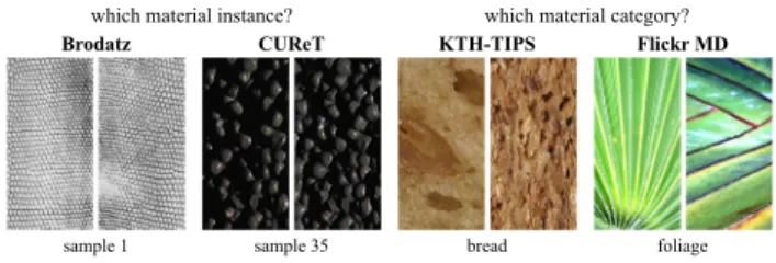
tex-Fig. 4 Datasets such asBrodatz(1966) and CUReT (Dana et al. 1999) (left) addressed the problem of material instance identification and oth-ers such as. KTH-T2b (Hayman et al. 2004) and FMD (Sharan et al. 2009) (right) addressed the problem of material category recognition. Our DTD dataset addresses a very different problem: the one of describ-ing a pattern usdescrib-ing intuitive attributes (Fig.1)

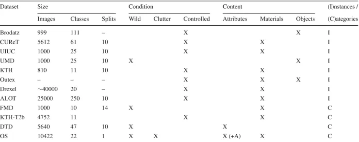
Table 1 Comparison of existing texture datasets, in terms of size, collection condition, nature of the classes to be recognized, and whether each class includes a single object/material instance or several instances of the same category

Dataset Size Condition Content (I)nstances /

Images Classes Splits Wild Clutter Controlled Attributes Materials Objects (C)ategories

Brodatz 999 111 – X X I CUReT 5612 61 10 X X I UIUC 1000 25 10 X X I UMD 1000 25 10 X X I KTH 810 11 10 X X I Outex – – – X X X I Drexel ∼40000 20 – X X I ALOT 25000 250 10 X X I FMD 1000 10 14 X X C KTH-T2b 4752 11 X X C DTD 5640 47 10 X X C OS 10422 22 1 X X X (+A) X C

Note that Outex is a meta-collection of textures spanning different datasets and problems

ture instances (e.g. matching half of the texture image given

the other half). Others includingCUReT(Dana et al. 1999),

UIUC(Lazebnik et al. 2005), KTH-TIPS (Caputo et al. 2005; Hayman et al. 2004),Outex(Ojala et al. 2002),Drexel Tex-ture Database(Oxholm et al. 2012), andALOT (Burghouts and Geusebroek 2009) address the recognition of specific instances of one or more materials.UMD(Xu et al. 2009) is similar, but the imaged objects are not necessarily composed of a single material. As textures are imaged under variable truncation, viewpoint, and illumination, these datasets have stimulated the creation of texture representations that are

invariant to viewpoint and illumination changes (Varma and

Zisserman 2005; Ojala et al. 2002; Varma and Zisserman 2003; Leung and Malik 2001). Frequently, texture under-standing is formulated as the problem of recognizing the material of an object rather than a particular texture instance (in this case any two slabs of marble would be considered

equal). KTH-T2b (Mallikarjuna et al. 2006) is one of the

first datasets to address this problem by grouping textures not only by the instance, but also by the type of materials (e.g. “wood”).

However, these datasets make the simplifying assumption that textures fill images, and often, there is limited intra-class

variability, due toa single or limited number of instances,

captured under controlled scale, view-angle and illumination. Thus, they are not representative of the problem of recog-nizing materials in natural images, where textures appear under poor viewing conditions, low resolution, and in clutter.

Addressing this limitation is the main goal of theFlickr

Mate-rial Database(FMD) (Sharan et al. 2009). FMD samples just one viewpoint and illumination per object, but contains many different object instances grouped in several different

mate-rial classes. Sect. 3 will introduce datasets addressing the

problem of clutter as well.

The performance of recognition algorithms on most of this data is close to perfect, with classification accuracies well above 95 %; KTH-T2b and FMD are an exception due to their increased complexity. A review of these datasets and

classification methodologies is presented inTimofte and Van

Gool(2012), who also propose a training-free framework to

classify textures, significantly improving on other methods.

Table1and Fig.4provides a summary of the nature and size

of various texture datasets that are used in our experiments.

3 Recognizing Textures in Clutter

This section looks at the second contribution of the paper, namely studying the recognition of materials and describable textures attributes not only “in the wild,” but also “in clutter”. Even in datasets such as FMD and DTD, in fact, each texture instance fills the entire image, which doest not match most applications. This section removes this limitation and looks at the problem of recognizing textures imaged in the larger context of a complex natural scene, including the challenging task of automatically segmenting textured image regions.

Rather than collecting a new image dataset from scratch,

our starting point is the excellentopen surfaces(OS) dataset

that was recently introduced by Bell et al. (2013). OS

comprises 25,357 images, each containing a number of high-quality texture/material segments. Many of these segments are annotated with additional attributes such as the material, viewpoint, BRDF estimates, and object class. Experiments focus on the 58,928 segments that contain material

anno-tations. Since material classes are highly unbalanced, we consider only the materials that contain at least 400 examples. This results in 53,915 annotated material segments in 10,422

images spanning 23 different classes.2Images are split evenly

into training, validation, and test subsets with 3474 images each. Segment sizes are highly variable, with half of them

being relatively small, with an area smaller than 64×64

pixels. One issue with crowdsourced collection of segmen-tations is that not all the pixels in an image are labelled. This makes it difficult to define a complete background class. For our benchmark several less common materials (includ-ing for example segments that annotators could not assign to a material) were merged in an “other” class that acts as the background.

This benchmark is similar to the one concurrently

pro-posed by Bell et al. (2015). However, in order to study

perceptual properties as well as materials, we also augment the OS dataset with some of the describable attributes of

Sect.2. Since the OS segments do not trigger with sufficient

frequency all the 47 attributes, the evaluation is restricted to eleven of them for which it was possible to identify at

least 100 matching segments.3The attributes were manually

labelled in the 53,915 segments retained for materials. We refer to this data as OSA.

3.1 Benchmark Tasks

As for DTD, the aim is to define standardized image under-standing tasks to be used as public benchmarks. The complete list of images, segments, labels, and splits are publicly

avail-able athttp://www.robots.ox.ac.uk/~vgg/data/wildtex/.

The benchmarks include two tasks on two

complemen-tary semantic domains. The first task is therecognition of

texture regions, given the region extent as ground truth infor-mation. This task is instantiated for both material, denoted

OS+R, and describable texture attributes, denoted OSA+R.

Performance in OS+R is measured in term of

classifi-cation accuracy and mAP, using the same definition (1)

where images are replaced by image regions. Performance in OSA+R uses instead mAP due to the possibility of multiple labels.

The second task is thesegmentation and recognition of

texture regions, which we also instantiate for materials (OS) and describable texture attributes (OSA). Since not all image

2_{The classes and corresponding number of example segments are: brick}

(610), cardboard (423), carpet/rug (1975), ceramic (1643), concrete (567), fabric/cloth (7484), food (1461), glass (4571), granite/marble (1596), hair (443), other (2035), laminate (510), leather (957), metal (4941), painted (7870), paper/tissue (1226), plastic/clear (586), plas-tic/opaque (1800), stone (417), tile (3085), wallpaper (483), wood (9232).

3_{These are: banded, blotchy, checkered, flecked, gauzy, grid, marbled,}

paisley, pleated, stratified, wrinkled.

pixels are labelled in the ground truth, the performance of

a predictorcˆis measured in term of per-pixel classification

accuracy, pp-acc(cˆ). This is computed using the same

for-mula as (1) with two modification: first, the images x are

replaced by pixelsp(extracted from all images in the dataset);

second, the ground truth labelc(p)of a pixel may take an

additional value 0 to denote pixels that are not labelled in the ground truth (the effect is to ignore them in the computation of accuracy).

In the case of OSA, the per-pixel accuracy is modified such that a class prediction is considered correct if it belongs to any of the ground-truth pixel labels. Furthermore, accuracy is not normalized per class as this is ill-defined, but by the total number of pixels:

acc-osa(cˆ)=|{p: ˆc(p)∈c(p)}|

|{p:c(p)=φ}| . (2)

where c(p)is the set of possible labels of pixel p and φ

denotes the empty set.

4 Texture Representations

Having presented our contributions to framing the problem of texture description, we now turn to our technical advances towards addressing the resulting problems. We start by revis-iting the concept of texture representation and studies how it relates to modern image descriptors based on CNNs. In general, a visual representation is a map that takes an image

x to a vectorφ(x) ∈ Rd that facilitates understanding the

image content. Understanding is often achieved by learning

a linear predictor φ(x),wscoring the strength of

associa-tion between the image and a particular concept, such as an object category.

Among image representations, this paper is particularly

interested in the class of texture representationspioneered

by the works of Mallat(1989),Malik and Perona (1990),

Bovik et al.(1990), andLeung and Malik(2001). Textures encompass a large diversity of visual patterns, from regular repetitions such as wallpapers, to stochastic processes such as fur, to intermediate cases such as pebbles. Distortions due to viewpoint and other imaging factors further complicate mod-eling textures. However, one can usually assume that, given a particular texture, appearance variations are statistically independent in the long range and can therefore be eliminated by averaging local image statistics over a sufficiently large texture sample. Hence, the defining characteristic of texture representations is to pool information extracted locally and uniformly from the image, by means of local descriptors, in an orderless manner.

The importance of texture representations is in the fact that they were found to be applicable well beyond textures. For

example, until recently many of the best object categorization

methods in challenges such as PASCAL VOC (

Evering-ham et al. 2007) and ImageNet ILSVRC (Deng et al. 2009) were based on variants of texture representations, developed specifically for objects. One of the contributions of this work is to show that these object-optimized texture representations are in fact optimal for a large number of texture-specific

prob-lems too (Sect.6.1.3).

More recently, texture representations have been

signif-icantly outperformed by Convolutional Neural Networks

(CNNs) in object categorization (Krizhevsky et al. 2012),

detection (Girshick et al. 2014), segmentation (Hariharan

et al. 2014), and in fact in almost all domains of image understanding. Key to the success of CNNs is their ability

to leverage largelabelleddatasets to learn high-quality

fea-tures. Importantly, CNN features pre-trained on very large datasets were found to transfer to many other domains with

a relatively modest adaptation effort (Jia 2013;Oquab et al.

2014; Razavin et al. 2014; Chatfield et al. 2014;Girshick et al. 2014). Hence, CNNs provide general-purpose image descriptors.

While CNNs generally outperform classical texture rep-resentations, it is interesting to ask what is the relation between these two methods and whether they can be

fruit-fully hybridized. Standard CNN-based methods such asJia

(2013),Oquab et al.(2014),Razavin et al.(2014),Chatfield et al.(2014), andGirshick et al.(2014) can be interpreted as extracting local image descriptors (performed by the the so called “convolutional layers”) followed by pooling such features in a global image representation (performed by the “Fully-Connected (FC) layers”). Here we will show that replacing FC pooling with one of the many pooling mechanisms developed in texture representations has several advantages: (i) a much faster computation of the represen-tation for image subregions accelerating applications such

as detection and segmentation (Girshick et al. 2014; He

et al. 2014; Gong et al. 2014), (ii) a significantly superior recognition accuracy in several application domains and (iii) the ability of achieving this superior performance without fine-tuning CNNs by implicitly reducing the domain shift problem.

In order to systematically study variants of texture

repre-sentationsφ=φe◦φf , we break them into local descriptor

extraction φf followed by descriptor pooling φe. In this

manner, different combinations of each component can be evaluated. Common local descriptors include linear filters, local image patches, local binary patterns, densely-extracted SIFT features, and many others. Since local descriptors are extracted uniformly from the image, they can be seen as

banks of (non-linear) filters; we therefore refer to them as

fil-ter banksin honor of the pioneering works ofMallat(1989), Bovik et al.(1990),Freeman and Adelson(1991),Leung and Malik(2001) and others where descriptors were the output

of actual linear filters. Pooling methods include bag-of-visual-words, variants using soft-assignment, or extracting higher-order statistics as in the Fisher vector. Since these methods encode the information contained in the local

descriptors in a single vector, we refer to them as pooling

encoders.

Sects.4.1and4.2discuss filter banks and pooling encoders

in detail.

4.1 Local Image Descriptors

There is a vast choice of local image descriptors in texture representations. Traditionally, these features were hand-crafted , but with the latest generation of deep learning methods it is now customary to learn them from data (although often in an implicit form). Representative exam-ples of these two families of local features are discussed in

Sects.4.1.1and4.1.2, respectively.

4.1.1 Hand-Crafted Local Descriptors

Some of the earliest local image descriptors were developed as linear filter banks in texture recognition. As an evolution

of earlier texture filters (Bovik et al. 1990;Malik and

Per-ona 1990), the filter bank of Leung Malik(LM)Leung and Malik(2001) includes 48 filters matching bars, edges and spots, at various scales and orientations. These filters are first and second derivatives of Gaussians at 6 orientations and 3 scales (36), 8 Laplacian of Gaussian (LOG) filters, and 4 Gaussians. Combinations of the filter responses, identified

by vector quantisation (Sect.4.2.1), were used as the

compu-tational basis of the “textons” proposed byJulesz and Bergen

(1983). The filter bankMR8ofVarma and Zisserman(2003)

andGeusebroek et al.(2003) consists instead of 38 filters, similar to LM. For two of the oriented filters, only the max-imum response across the scales is recorded, reducing the number of responses to 8 (3 scales for two oriented filters, and two isotropic – Gaussian and Laplacian of Gaussian).

The importance of using linear filters as local features was

later questioned by Varma and Zisserman(2003). The VZ

descriptors are in fact small image patches which, remark-ably, were shown to outperform LM and MR8 on earlier texture benchmarks such as CuRET. However, as will be demonstrated in the experiments, trivial local descriptors are not competitive in harder tasks.

Another early local image descriptor are theLocal Binary

Patterns(LBP) ofOjala et al.(1996) andOjala et al.(2002),

a special case of the texture units ofWang and He(1990). A

LBPdi =(b1, . . . ,bm)computed a pixelp0is the sequence

of bitsbj = [x(pi) >x(pj)]comparing the intensityx(pi)

of the central pixel to the one ofmneighborspj (usually 8

in a circle). LBPs have specialized quantization schemes; the

uniform patterns(Ojala et al. 2002). The quantized LBPs can be averaged over the image to build a histogram; alternatively, such histograms can be computed for small image patches and used in turn as local image descriptors.

In the context of object recognition, the best known local

descriptor is undoubtedly Lowe’sSIFT(Lowe 1999). SIFT

is the histogram of the occurrences of image gradients quan-tized with respect to their location within a patch as well to their orientation. While SIFT was originally introduced to match object instances, it was later applied to an impres-sive diversity of tasks, from object categorization to semantic segmentation and face recognition.

4.1.2 Learned Local Descriptors

Handcrafted image descriptors are nowadays outperformed by features learned using the latest generation of deep

CNNs (Krizhevsky et al. 2012). A CNN can be seen as a

compositionφK◦ · · · ◦φ2◦φ1ofKfunctions orlayers. The

output of each layerxk =(φk◦· · ·◦φ2◦φ1)(x)is adescriptor

fieldxk ∈RWk×Hk×Dk, whereWkandHkare the width and

height of the field andDkis the number of feature channels.

By collecting theDk responses at a certain spatial location,

one obtains aDkdimensional descriptor vector. The network

is called convolutional if all the layers are implemented as (non-linear) filters, in the sense that they act locally and uni-formly on their input. If this is the case, since compositions of

filters are filters, the feature fieldxkis the result of applying

a non-linear filter bank to the imagex.

As computation progresses, the resolution of the descrip-tor fields decreases whereas the number of feature channels

increases. Often, the last several layersφkof a CNN are called

“fully connected” because, if seen as filters, their support is

the same as the size of the input fieldxk−1and therefore lack

locality. By contrast, earlier layers that act locally will be

referred to as “convolutional”. If there areCconvolutional

layers, the CNNφ=φe◦φf can be decomposed into a filter

bank (local descriptors)φf =φC◦ · · · ◦φ1followed by a

pooling encoderφe=φK◦ · · · ◦φC+1.

4.2 Pooling Encoders

A pooling encoder takes as input the local descriptors

extracted from an imagex and produces as output a single

feature vectorφ(x), suitable for tasks such as classification

with an SVM. A first important differentiating factor between encoders is whether they discard the spatial configuration

of input features (orderless pooling; Sect.4.2.1) or whether

they retain it (order-sensitive pooling; Sect.4.2.2). A detail

of practical importance, furthermore, is the type of post-processing applied to the pooled vectors (post-post-processing;

Sect.4.2.3).

4.2.1 Orderless Pooling Encoders

An orderless pooling encoder φe maps a sequence F =

(f1, . . . ,fn),fi ∈RDof local image descriptors to a feature

vectorφe(F) ∈ Rd. The encoder is orderless in the sense

that the functionφeis invariant to permutations of the input

F.4Furthermore, the encoder can be applied to any number

of features; for example, the encoder can be applied to the

sub-sequenceF⊂Fof local descriptors contained in a

tar-get image region without recomputing the local descriptors themselves.

All common orderless encoders are obtained by applying

a non-linear descriptor encoder η(fi) ∈ Rd to individual

local descriptors and then aggregating the result by using a commutative operator such as average or max. For example,

average-pooling yieldsφ¯e(F)= 1_n

n

i=1η(fi). The pooled

vectorφ¯e(F)is post-processed to obtain the final

represen-tationφe(F)as discussed later.

The best-known orderless encoder is the Bag of Visual

Words (BoVW). This encoder starts by vector-quantizing

(VQ) the local featuresfi ∈ RDby assigning them to their

closestvisual wordin a dictionaryC=c1. . .cd

∈RD×d

of d elements. Visual words can be thought of as

“proto-type features” and are obtained during training by clustering

example local features. The descriptor encoderη1(fi)is the

one-hot vector indicating the visual word corresponding to

fi and average-pooling these one-hot vectors yields the

his-togram of visual words occurrences. BoVW was introduced

in the work ofLeung and Malik(2001) to characterize the

distribution of textons, defined as configuration of local filter responses, and then ported to object instance and category

understanding by Sivic and Zisserman (2003) and Csurka

et al. (2004) respectively. It was then extended in several ways as described below.

The kernel codebook encoder (Philbin et al. 2008) assigns

each local feature to several visual words, weighted by a

degree of membership: [ηKC(fi)]j ∝ exp

−λfi−cj2

,

whereλis a parameter controlling the locality of the

assign-ment. The descriptor codeηKC(fi)isL1normalized before

aggregation, such that ηKC(fi)1 = 1. Several related

methods used concepts from sparse coding to define the

local descriptor encoder (Zhou et al. 2010;Liu et al. 2011).

Locality constrained linear coding (LLC) (Wang et al.

2010), in particular, extends soft assignment by making the

assignments reconstructive, local, and sparse: the descriptor

encoderηLLC(fi)∈Rd₊,ηLLC(fi)1=1,ηLLC(fi)0 ≤r

is computed such thatfi ≈CηLLC(fi)while allowing only

therd visual words closer tofi to have a non-zero

coef-fcient.

4 _{Note thatFcannot be represented as a set as encoders are generally}

sensitive to repetitions of feature descriptors. It could be defined as a multiset or, as done here, as a sequenceF.

In theVector of locally-aggregated descriptors(VLAD) (Jégou et al. 2010) the descriptor encoder is richer. Local image descriptors are first assigned to their nearest

neigh-bor visual word in a dictionary of K elements like in

BoVW; then the descriptor encoder is given byηVLAD(fi)=

(fi −Cη1(fi))⊗η1(fi), where⊗is the Kronecker product.

Intuitively, this subtracts fromfi the corresponding visual

word Cη1(fi) and then copies the difference into one of

K possible subvectors, one for each visual word. Hence

average-poolingηVLAD(fi)accumulates first-order

descrip-tor statistics instead of simple occurrences as in BoVW.

VLAD can be seen as a variant of the Fisher vector

(FV) (Perronnin and Dance 2007). The FV differs from

VLAD as follows. First, the quantizer is not K-means

but a Gaussian Mixture Model (GMM) with components (πk, μk, k), k = 1, . . . ,K, where πk ∈ Ris the prior

probability of the component, μk ∈ RD the Gaussian

mean andk ∈ RD×D the Gaussian covariance (assumed

diagonal). Second, hard-assignmentsη1(fi)are replaced by

soft-assignmentsηGMM(fi)given by the posterior probability

of each GMM component. Third, the FV descriptor encoder

ηFV(fi)includes both first−

1 2

k (fi −μk)and second order

−1

k (fi−μk)(fi−μk)−1statistics, weighted byηGMM(fi)

[seePerronnin and Dance(2007),Perronnin et al.(2010) and Chatfield et al.(2011) for details]. Hence, average pooling

ηFV(fi)accumulates both first and second order statistics of

the local image descriptors.

All the encoders discussed above use average pooling, except LLC that uses max pooling.

4.2.2 Order-Sensitive Pooling Encoders

Anorder-sensitive encoderdiffers from an orderless encoder

in that the mapφe(F)is not invariant to permutation of the

inputF. Such an encoder can therefore reflect the layout

of the local image desctiptors, which may be ineffective or even counter-productive in texture recognition, but is usually helpful in the recognition of objects, scenes, and others.

The most common order-sensitive encoder method is the spatial pyramid pooling(SPP) of Lazebnik et al.(2006). SSP transforms any orderless encoder into one with (weak) spatial sensitivity by dividing the image in subregions, com-puting any encoder for each subregion, and stacking the results. This encoder is only be sensitive to reassignments of the local descriptors to different subregions.

The fully-connected layers (FC) in a CNN also form an order-sensitive encoder. Compared to the encoders seen above, FC are pre-trained discriminatively, which can be either an advantage or disadvantage, depending on whether the information that they captured can be transferred to the domain of interest. FC poolers are much less flexible than the encoders seen above as they work only with a particular type

of local descriptors, namely the corresponding CNN convo-lutional layers. Furthermore, a standard FC pooler can only operate on a well defined layout of local descriptors (e.g. a 6×6), which in turn means that the image needs to be resized to a standard size before the FC encoder can be evaluated. This is particularly expensive when, as in object detection or image segmentation, many image subregions must be con-sidered.

4.2.3 Post-processing

The vector y = φe(F) obtained by pooling local image

descriptors is usually post-processed before being used in a classifier. In the simplest case, this amounts to performing

L2normalizationφe(F)=y/y2. However, this is usually

preceded by a non-linear transformationφK(y)which is best

understood in term of kernels. Akernel K(y,y)specifies a

notion ofsimilaritybetween data pointsyandy. IfK is a

positive semidefinite function, then it can always be rewritten

as the inner product φK(y), φK(y) where φK is a

suit-able pre-processing function called akernel embedding(Maji

et al. 2008;Vedaldi and Zisserman 2010). Typical kernels

include the linear, Hellinger’s, additive-χ2, and

exponential-χ2_{ones, given respectively by:}

y,y, d i=1 y_iy_i, d i=1 2y_iy_i y_i+y_i, exp −λ d i=1 (y_i−y_i)2 y_i+y_i .

In practice, the kernel embeddingφKcan be computed easily

only in a few cases, including the linear kernel (φK is the

identity) and Hellinger’s kernel (for each scalar component, φHell.(y) = √y). In the latter case, if y can take negative

values, then the embedding is extended to the so calledsigned

square rooting5φHell.(y)=sign(y)√|y|.

Even ifφK is not explicitly computed, any kernel can be

used to learn a classifier such as an SVM (kernel trick). In this

case, L2normalizing the kernel embeddingφK(y)amounts

to normalizing the kernel as

K(y,y)= K(y _,y)

K(y,y)K(y,y).

All the pooling encoders discussed above are usually

fol-lowed by post-processing. In particular, theImproved Fisher

Vector (IFV) (Perronnin et al. 2010) prescribes the use of

the signed-square root embedding followed by L2

normal-ization. VLAD has several standard variants that differ in

5 _{This extension generalizes to all homogeneous kernels, including for}

the post-processing; here we use the one thatL2normalizes the individual VLAD subvectors (one for each visual word)

beforeL2normalizing the whole vector (Arandjelovic and

Zisserman 2012).

5 Plan of Experiments and Highlights

The next several pages contain an extensive set of experimen-tal results. This section provides a guide to these experiments and summarizes the main findings.

The goal of the first block of experiments (Sect.6.1) is

to determine which representations work bests on different problems such as texture attribute, texture material, object, and scene recognition. The main findings are:

– Orderless pooling of SIFT features (e.g. FV-SIFT) per-forms better than specialized texture descriptors in many texture recognition problems; performance is further improved by switching from SIFT to CNN local

descrip-tors (FV-CNN; Sect.6.1.3).

– Orderless pooling of CNN descriptors using the Fisher Vector (FV-CNN) is often significantly superior than fully-connected pooling of the same descriptors (FC-CNN) in texture, scene, and object recognition

(Sect.6.1.4). This difference is more marked for deeper

CNN architectures (Sect. 6.1.5) and can be partially

explained by the ability of FV pooling to overfit less and to easily integrate information at multiple image scales

(Sect.6.1.6).

– FV-CNN descriptors can be compressed to the same dimensionality of FC-CNN descriptors while preserving

accuracy (Sect.6.1.7).

Having determined good representations in Sect.6.1, the

second block of experiments (Sect.6.2) compares them to

the state of the art in texture, object, and scene recognition. The main findings are:

– In texture recognition in the wild, for both materials (FMD) and attributes (DTD), CNN-based descriptors substantially outperform existing methods. Depending on the dataset, FV pooling is a little or substantially bet-ter than FC pooling of CNN descriptors (Sect. 6.2.1.4). When textures are extracted from a larger cluttered scene (instead of filling the whole image), the difference between FV and FC pooling increases (Sect. 6.2.1.5). – In coarse object recognition (PASCAL VOC),

fine-grained object recognition (CUB-200), scene recognition (MIT Indoor), and recognition of things & stuff (MSRC) fine-grained, the FV-CNN representation achieves results that are close and sometimes superior to the state of

the art, while using a simple and fully generic pipeline

(Sect.6.2.3).

– FV-CNN appears to be particularly effective in domain

transfer. Sect.6.2.3shows in fact that FV pooling

com-pensates for the domain gap caused by training a CNN on two very different domains, namely scene and object recognition.

Having addressed image classification in Sects.6.1and

6.2, The third block of experiments (Sect.7) compare

rep-resentations on semantic segmentation. It shows that FV pooling of CNN descriptors can be combined with a region proposal generator to obtain high-quality segmentation of materials in the OS and MSRC data. For example, combined with a post-processing step using a CRF, FV-VGG-VD sur-passes the state-of-the-art on the latter dataset. It is also shown that, differently from FV-CNN, FC-CNN is too slow to be practical in this scenario.

6 Experiments on Semantic Recognition

So far the paper has introduced novel problems in texture understanding as well as a number of old and new texture rep-resentations. The goal of this section is to determine, through extensive experiments, what representations work best for which problem.

Representations are labelled as pairs X-Y, where X is a pooling encoder and Y a local descriptor. For example, FV-SIFT denotes the Fisher vector encoder applied to densely extracted SIFT descriptors, whereas BoVW-CNN denotes the bag-of-visual-words encoder applied on top of CNN con-volutional descriptors. Note in particular that the CNN-based image representations as commonly extracted in the litera-ture Jia(2013),Razavin et al.(2014), andChatfield et al.

(2014) implicitly use CNN-based descriptors and the FC

pooler, and therefore are denoted here as FC-CNN. 6.1 Local Image Descriptors and Encoders Evaluation This section compares different local image descriptors and

pooling encoders (Sect. 6.1.1) on selected representative

tasks in texture recognition, object recognition, and scene

recognition (Sect. 6.1.2). In particular, Sect. 6.1.3

com-pares different local descriptors, Sect.6.1.4different pooling

encoders, and Sect. 6.1.5 additional variants of the

CNN-based descriptors.

6.1.1 General Experimental Setup

The experiments are centered around two types of local descriptors. The first type are SIFT descriptors extracted

are sampled with a step of two pixels and the support of the descriptor is scaled such that a SIFT spatial bin has size

8×8 pixels. Since there are 4×4 spatial bins, the

sup-port or “receptive field” of each DSIFT descriptor is 40×40

pixels, (including a border of half a bin due to bilinear

inter-polation). Descriptors are 128-dimensional (Lowe 1999), but

their dimensionality is further reduced to 80 using PCA, in all experiments. Besides improving the classification accu-racy, this significantly reduces the size of the Fisher Vector and VLAD encodings.

The second type of local image descriptors are deep

convolutional features (denoted CNN) extracted from the

convolutional layers of CNNs pre-trained on ImageNet ILSVRC data. Most experiments build on the VGG-M model ofChatfield et al.(2014) as this network performs better than

standard networks such as the Caffe reference model (Jia

2013) and AlexNet (Krizhevsky et al. 2012) while having a

similar computational cost. The VGG-M convolutional fea-tures are extracted as the output of the last convolutional layer, directly from the linear filters excluding ReLU and max pooling, which yields a field of 512-dimensional descrip-tor vecdescrip-tors. In addition to VGG-M, experiments consider the recent VGG-VD (very deep with 19 layers) model of Simonyan and Zisserman(2014). The receptive field of CNN

descriptors is much larger compared to SIFT: 139×139

pix-els for VGG-M and 252×252 for VGG-VD.

When combined with a pooling encoder, local descriptors are extracted at multiple scales, obtained by rescaling the

image by factors 2s,s = −3,−2.5, . . . ,1.5 (but, for

effi-ciency, discarding scales that would make the image larger

than 10242pixels).

The dimensionality of the final representation strongly

depends on the encoder type and parameters. ForK visual

words, BoVW and LLC haveKdimensions, VLAD hasK D

and FV 2K D, whereDis the dimension of the local

descrip-tors. For the FC encoder, the dimensionality is fixed by the CNN architecture; here the representation is extracted from the penultimate FC layer (before the final classification layer) of the CNNs and happens to have 4096 dimensions for all the CNNs considered. In practice, dimensions vary widely, with BoVW, LLC, and FC having a comparable dimensionality, and VLAD and FV a much higher one. For example, FV-CNN

has64·103dimensions with K =64 Gaussian mixture

components, versus the 4096 of FC, BoVW, and LLC (when

used with K = 4096 visual words). In practice, however,

dimensions are hardly comparable as VLAD and FV

vec-tors are usually highly compressible (Parkhi et al. 2014). We

verified that by using PCA to reduce FV to 4096 dimensions and observing only a marginal reduction in classification per-formance in the PASCAL VOC object recognition task, as described below.

Unless otherwise specified, learning uses a standard non-linear SVM solver. Initially, cross-validation was used to

select the parameterC of the SVM in the range{0.1,1,10,

100}; however, after noting that performance was nearly

identical in this range (probably due to the data

normaliza-tion),Cwas simply set to the constant 1. Instead, it was found

that recalibrating the SVM scores for each class improves classification accuracy (but of course not mAP). Recalibra-tion is obtained by changing the SVM bias and rescaling the SVM weight vector in such a way that the median scores of the negative and positive training samples for each class are

mapped respectively to the values−1 and 1.

All the experiments in the paper use the VLFeat library (Vedaldi and Fulkerson 2010) for the computation of SIFT features and the pooling embedding (BoVW, VLAD, FV).

The MatConvNet (Vedaldi and Lenc 2014) library is used

instead for all the experiments involving CNNs. Further details specific to the setup of each experiment are given below as needed.

6.1.2 Datasets and Evaluation Measures

The evaluation is performed on a diversity of tasks: the new describable attribute and material recognition benchmarks in DTD and OpenSurfaces, existing ones in FMD and KTH-T2b, object recognition in PASCAL VOC 2007, and scene recognition in MIT Indoor. All experiments follow standard evaluation protocols for each dataset, as detailed below.

DTD(Sect.2) contains 47 texture classes, one per visual

attribute, containing 120 images each. Images are equally spilt into train, test and validation, and include experi-ments on the prediction of “key attributes” as well as “joint

attributes”, as as defined in Sect.2.1, and reports accuracy

averaged over the 10 default splits provided with the datasets. OpenSurfaces(Bell et al. 2013) is used in the setup described

in Sect. 3 and contains 25,357 images, out of which we

selected 10,422 images, spanning across 21 categories. When segments are provided, the dataset is referred to as OS+R, and recognition accuracy is reported on a per-segment basis. We also annotated the segments with the attributes from DTD, and called this subset OSA (and OSA+R for the setup when segments are provided). For the recognition task on OSA+R we report mean average precision, as this is a multi-label dataset.

FMD(Sharan et al. 2009) consists of 1,000 images with 100 for each of ten material categories. The standard

evalua-tion protocol ofSharan et al.(2009) uses 50 images per class

for training and the remaining 50 for testing, and reports

clas-sification accuracy averaged over 14 splits.KTH-T2b[65]

contains 4,752 images, grouped into 11 material categories. For each material category, images of four samples were captured under various conditions, resulting in 108 images

per sample. Following the standard procedure (Caputo et al.

2005; Timofte and Van Gool 2012), images of one mater-ial sample are used to train the model, and the other three

samples for evaluating it, resulting in four possible splits of the data, for which average per-class classification

accu-racy is reported.MIT Indoor Scenes(Quattoni and Torralba

2009) contains 6,700 images divided in 67 scene categories.

There is one split of the data into train (80 %) and test (20 %), provided with the dataset, and the evaluation metric

is average per-class classification accuracy.PASCAL VOC

2007(Everingham et al. 2007) contains 9963 images split across 20 object categories. The dataset provides a stan-dard split in training, validation and test data. Performance is reported in term of mean average precision (mAP) computed

using the TRECVID 11-point interpolation scheme (

Evering-ham et al. 2007).6

6.1.3 Local Image Descriptors and Kernels Comparison The goal of this section is to establish which local image descriptors work best in a texture representation. The ques-tion is relevant because: (i) while SIFT is the de-facto standard handcrafted-feature in object and scene recognition, most authors use specialized descriptors for texture recogni-tion and (ii) learned convolurecogni-tional features in CNNs have not yet been compared when used as local descriptors (instead, they have been compared to classical image representations when used in combination with their FC layers).

The experiments are carried on the the task of

recogniz-ing describable texture attributes in DTD (Sect.2) using the

BoVW encoder. As a byproduct, the experiments determine the relative difficulty of recognizing the different 47 percep-tual attributes in DTD.

6.1.3.1 Experimental Setup The following local image

descriptors are compared: the linear filter banks ofLeung and

Malik(LM) (Leung and Malik 2001) (48D descriptors) and

MR8(8D descriptors) (Varma and Zisserman 2005;

Geuse-broek et al. 2003), the 3×3 and 7×7 raw image patches ofVarma and Zisserman(2003) (respectively 9D and 49D), thelocal binary patterns(LBP) ofOjala et al.(2002) (58D),

SIFT (128D), and CNN features extracted fromVGG-Mand

VGG-VD(512D).

After the BoVW representation is extracted, it is used to train a 1-vs-all SVM using the different kernels

dis-cussed in Sect. 4.2.3: linear, Hellinger, additive-χ2, and

exponential-χ2. Kernels are normalized as described before.

The exponential-χ2kernel requires choosing the parameter

λ; this is set as the reciprocal of the mean of theχ2distance

matrix of the training BoVW vectors. Before computing the

exponential-χ2 kernel, furthermore, BoVW vectors are L1

normalized. An important parameter in BoVW is the

num-ber of visual words selected.K was varied in the range of

6_{The procedure for computing the AP was changed in later versions}

of the benchmark.

256, 512, 1024, 2048, 4096 and performance evaluated on a validation set. Regardless of the local feature and embedding,

performance was found to increase with K and to saturate

aroundK =4096 (although the relative benefit of increasing

Kwas larger for features such as SIFT and CNNs). Therefore

K was set to this value in all experiments.

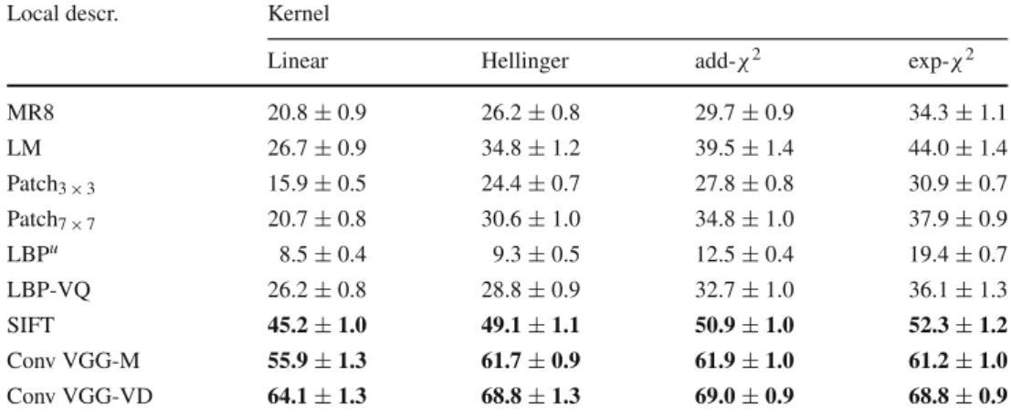
6.1.3.2 Analysis Table2reports the classification accuracy

for 47 1-vs-all SVM attribute classifiers, computed as (1). As

often found in the literature, the best kernel was found to be

exponential-χ2_{, followed by additive-χ}2_{, Hellinger’s, and}

linear kernels. Among the hand-crafted descriptors, dense SIFT significantly outperforms the best specialized texture

descriptor on the DTD data (52.3 % for BoVW-exp-χ2

-SIFT vs 44 % for BoVW-exp-χ2-LM). CNN local descriptors

handily outperform handcrafted features by a 10–15 % recog-nition accuracy margin. It is also interesting to note that the choice of kernel function has a much stronger effect for image patches and linear filters (e.g. accuracy nearly doubles

mov-ing from BoVW-linear-patches to BoVW-exp-χ2-patches)

and an almost negligible effect for the much stronger CNN features.

Figure 5 reports the classification accuracy for each

attribute in DTD for the BoVW-SIFT, BoVW-VGG-M, and

BoVW-VGG-VD descriptors and the additive-χ2kernel. As

it may be expected, concepts such aschequered,waffled,

knit-ted,paisleyachieve nearly perfect classification, while others

such asblotchy,smearedorstainedare far harder.

6.1.3.3 Conclusions The conclusions are that (i) SIFT descriptors outperform significantly texture-specific descrip-tors such as linear filter banks, patches, and LBP on this texture recognition task, and that (ii) learned convolutional local descriptors significantly surpass SIFT.

6.1.4 Pooling Encoders

The previous section established the primacy of SIFT and CNN local image descriptors on alternatives. The goal of this

section is to determine which pooling encoders (Sect. 4.2)

work best with these descriptors, comparing the orderless BoVW, LLC, VLAD, FV encoders and the order-sensitive FC encoder. The latter, in particular, reproduces the CNN transfer learning setting commonly found in the literature where CNN features are extracted in correspondence to the FC layers of a network.

6.1.4.1 Experimental Setup The experimental setup is sim-ilar to the previous experiment: the same SIFT and CNN VGG-M descriptors are used; BoVW is used in combination with the Hellinger kernel (the exponential variant is slightly

better, but much more expensive); the same K = 4096