A Deep Learning Model for Personalized Human Activity Recognition

A Deep Learning Model for Personalised

Human Activity Recognition

Student: Davide

_Buffelli

Advisor: Prof. Fabio

_Vandin

Academic Year 2018-2019

Master of Science in Computer Engineering

Università degli Studi di Padova

Abstract

Human Activity Recognition (HAR) is a time series classification task that involves predicting the movement or action of a person based on sensor data (for example, for fitness tracking applications). In the past the problem has been tackled by hand crafting features, which is time consuming and doesn’t generalize well. In this thesis we firstly analyze a Deep Learning model created for Time Series data that has set the state of the art in HAR on smartphones and wearable devices (using data from accelerometer and gyroscope), and we test the benefits of Data Augmentation as a technique to add robustness against noise. We then propose a customized version of the framework that is capable of adapting over time to a specific user, improving the accuracy of its predictions. We show the effectiveness of the proposed framework by testing its learning capabilities and evaluating the improvements on the accuracy of the predictions.

Contents

Notation iv

1 Introduction 1

2 Deep Learning Tools 7

2.1 Neural Networks and the Backpropagation Algorithm . . . 7

2.2 Adam Optimizer . . . 9

2.3 Convolutional Neural Networks . . . 10

2.4 Recurrent Neural Networks . . . 15

2.5 Dropout . . . 18 2.6 L2 Regularization . . . 19 2.7 Batch Normalization . . . 20 3 DeepSense Architecture 23 3.1 Data Pre-Processing . . . 25 3.2 CNN Layers . . . 26 3.2.1 Individual Layers . . . 27 3.2.2 Merge Layers . . . 28 3.3 RNN Layers . . . 29 3.4 Output Layer . . . 29

3.5 Loss Function and Regularization . . . 30

4 Customizing DeepSense 31 5 Experimental Tools & Settings 35 5.1 TensorFlow . . . 36 5.2 Tests . . . 38 6 Results 41 7 Conclusions 46 7.1 Future Work . . . 46 Bibliography 47

Notation

This section will describe the notation used throughout this thesis. Given it’s simplicity and clarity, we decided to adopt the notation defined by GoodFellow, Bengio and Courville, in their book “Deep Learning” [1].

Numbers & Arrays

x A scalar (integer or real)

x A vector

X A matrix

X A tensor

Indexing

xi i-th element of vector x

Xi,j Element (i, j) of matrix X Xi,j,k Element (i, j, k) of tensor X

X:,:,k k-th 2-D slice of a 3-D tensorX

We will use a zero-based numbering for the indexes of vectors and matrices. This means that the elements of an array of size n will have indexes that go from 0 to n−1. Similarly, the rows and columns of an×m matrix go from 0 to n−1

and from 0 tom−1.

Sets

X A set

Chapter 1

Introduction

Modern devices, like smartphones and smartwatches, are equipped with several sen-sors, like accelerometer, gyroscope, barometer, and magnetometer. This sensors are used for a large variety of tasks that we can identify as regression or classifi-cation. Regression tasks consist in all those problems where the output variable (what we want to obtain or predict) takes continuous values. An example is a map application that changes the orientation of the map based on what direction you’re facing. The direction changes in a continuous way and can be represented with a real value that describes an angle. Classification tasks instead, consist in all those problems where we want to identify a group membership. An example is when the measurements of the sensors inside of a smartphone are used to obtain the orientation of the device, in order to adapt the user interface. In this case we only have four classes (landscape right, landscape left, portrait up, portrait down) and we want to identify the correct one in a given moment.

The biggest problem with on-device sensors is that their measurements are noisy and it’s difficult to find a distribution that precisely describes the noise. For regression tasks, we usually rely on physical models, but this means that the accu-racy of our predictions is only as good as the noise assumptions. For classification tasks the common practice is to use manually designed features, but this requires a lot of experiments and there is no guarantee that the features will work well with new users.

This thesis will analyze the DeepSense architecture proposed by Yao et al. [2], whose aim is to improve the accuracy of mobile sensor exploitation. This ar-chitecture defines a deep learning framework that combines convolutional neural networks and recurrent neural networks, and that is able to “exploit local inter-actions among similar mobile sensors, merge local interinter-actions of different sensory modalities into global interactions, and extract temporal relationships to model sig-nal dynamics”. To demonstrate the effectiveness of DeepSense the authors showed that it outperforms state of the art methods for three different tasks:

• Car tracking with motion sensors: the goal here is to determine the position of a car, with respect to a starting point, using only acceleration measurements obtained by an accelerometer.

• Heterogeneous Human Activity Recognition: the task consists in de-tecting the activity (like “walking” or “cycling” for example) that a user is

performing, taking advantage of data from the accelerometer and the gyro-scope installed on a smartphone or a wearable device.

• User identification with biometric motion analysis: the idea is to uniquely identify a user by his “walking style” (again by using data from accelerometer and gyroscope obtained from a smartphone).

In the article the authors show that DeepSense is able to excel in all three tasks. In this thesis we will focus only onHeterogeneous Human Activity Recognition be-cause, of the three, it is the only one that is actually used in real-world commercial applications. In fact all modern smartphones, smartwatches and fitness trackers implement some kind of activity recognition system and this implies that an im-provement in this field can have a big impact in devices that are used by millions of people.

We will now describe the dataset that has been used in the experimental part of this thesis (the same used by Yao et al. [2]) and we will explore some of the previous work that has been done on the Human Activity Recognition problem. In Chapter 2 we will explain all the deep learning structures and techniques that are necessary to understand the DeepSense framework. In Chapter 3 we will present the DeepSense framework in all its details, from both a theoretical and a practical point of view. Chapter 4 presents the custom model we created to improve the performances of DeepSense. Chapter 5 describes the experimental work that has been done for this thesis; we will describe all the tools and the settings that we adopted, the principal libraries used to write the code, and the the tests that have been done. In Chapter 6 we will show the results we obtained from the tests and finally in Chapter 7 we will discuss them and we will present some future work.

HHAR Dataset

The Heterogeneity Human Activity Dataset (HHAR) was first introduced in a paper by Stisen et al. [3], and is available for download from the UCI Machine Learning Repository1. The dataset is composed by data from two different experi-ments, one where the device used for the measurements were positioned according to some specific orientation and one were the orientation of the devices was not specified. We will use the data from the second experiment (as it is done by the authors in the DeepSense paper) because we want to be able to identify a specific activity independently from how the device is positioned.

The activities that were considered are 6: “Biking”, “Sitting”, “Standing”, “Walk-ing”, “Stair Up” and “Stair Down”. For the measurements, accelerometer and gy-roscope were sampled at the highest possible frequency. The data was taken from 8 smartphones (2 Samsung Galaxy S3 mini, 2 Samsung Galaxy S3, 2 LG Nexus 4, 2 Samsung Galaxy S+) and 4 smartwatches (2 LG watches, 2 Samsung Galaxy Gears), used by 9 different users. In particular each user performed all of the 6 activities with all the devices (one at a time). As done by the authors of the DeepSense paper, we will only consider the data obtained from smartphones.

1

The data is split into 4 .csv files divided by device (phone or watch), and sen-sor (gyroscope and accelerometer). Each.csv file consists of the following columns: Index Arrival Time Creation Time x y z User Model Device Ground Truth

Each field of the .csv file is described in Table 1.1.

Index Number of the row in the file.

Arrival Time The timestamp of when the measurement arrived to the sensing application.

Creation Time The timestamp the OS attaches to the sample. x The value provided by the sensor for the x axis. y The value provided by the sensor for the y axis. z The value provided by the sensor for the z axis.

User The user that generated this sample (a character from ‘a’ to ‘i’).

Model A string identifying the phone or watch model that generated this sample.

Device A string identifying the specific phone or watch that generated this sample (necessary to distinguish between two or more de-vices of the same model).

Ground Truth A string identifying the activity that was being executed by the user when this sample was taken (“Biking”, “Sitting”, “Stand-ing”, “Walk“Stand-ing”, “Stair Up” or “Stair Down”).

Table 1.1

Previous Work

The human activity recognition problem has been extensively studied in the past and various datasets are available online. Previous work tackled the problem by hand-crafting features (see [3] and [4]), but this requires a lot of experiments (and time) and it is not guaranteed to generalize well.

Figo et al. [4] published a survey analysing the most representative domain approaches and techniques. The three domains identified by the authors are:

• Time Domain: the techniques in this domain try to extract basic signal information from raw sensor data. To perform this task mathematical/sta-tistical functions are used (mean, variance, standard variation, root mean square, cross correlation, etc.) and other functions like angular velocity, dif-ferences, signal magnitude area, signal vector magnitude, etc. Sometimes these measures have been used as the base for machine learning techniques like neural networks and support vector machines.

• Frequency Domain: in this case the raw signal is first transformed using the Fourier transform and then the features are extracted from the frequency-domain representation of the signal. Some of the most used features are:

DC component, spectral energy, information entropy, spectral coefficients. Another technique in the frequency domain that doesn’t use the Fourier transform is the Wavelet analysis.

• Symbolic Strings Domain: here the idea is to transform accelerometer and other sensors’ signals into strings of discrete symbols. A typical way of performing this task is to split the signal into windows of w consecutive samples and then apply some kind of averaging and discretization to obtain a value from a fixed sized alphabet. Once the signal has been transformed into a string, it is possible to compute some metrics like Euclidian-related distances, Levenshtein Edit distance or Dynamic Time Warping (DTW). In the survey the authors analysed the computational complexity, storage costs and memory operations and they studied the “suitability” of each technique for mobile devices. Finally they performed some experiments to measure the accuracy of the different methods. The results obtained showed that Frequency domain techniques, on average, perform the best with an accuracy of 70.1% on the test set.

Stisen et al. [3] conducted experiments with 36 smartphones and smartwatches (consisting of 13 different device models from four manufacturers) using the most popular feature representation and classification techniques for HAR. In this study the authors analysed also methods based on the empirical cumulative distribu-tion funcdistribu-tion (ECDF), that were not considered in the work by Figo et al. These experiments showed that the sensor biases, the sample rate instability and hetero-geneity of the different devices have a huge impact on classification results. The authors also proposed some mitigation techniques, in the form of pre-processing methods that seem to be effective but they also add more load to the CPU. In the end the authors concluded that ECDF and time based features are the most recommended, but it is clear that hand-crafted features are not the best solution for human activity recognition.

With the recent “explosion” of Deep Learning, some studies tried to approach the HAR problem with these technique. In fact, Deep Learning can automate the extraction of features, and this has been done, for user identification, in a system called IDNet proposed by Rossi and Gadaleta [5]. In more detail, IDNet is com-posed by a first part that receives the raw data form the sensors and transforms it into an orientation independent reference system, in order to eliminate the im-pacts of disorientation and misplacement errors. Then there is a time interpolation process (to remove sampling rate instabilities) and some noise elimination. After this the authors developed an algorithm that identifies walking cycles, which are then fed into a Convolutional Neural Network for feature extraction. The output is then classified using support vector machines because the goal of IDNet is to identify a user from it’s “walking style”. We can notice that IDNet had a lot of “traditional” algorithms and only a small part of deep learning. DeepSense instead is based entirely on deep learning. In fact, as we will see, all the parts of the system are learned from the data used to train the architecture. Other kinds of Deep Learning networks have also been used for HAR. For example, Radu et al. [6] proposed a system based on Restricted Boltzman Machines (RBMs) [7]. In more detail they created a structure with two hidden layers per sensor and a final hidden

layer that combines the data obtained from the different sensors (this architecture, as we will see, is similar to how DeepSense works). This fairly simple structure obtained an accuracy of circa 80% on the test set, showing that Deep Learning is a very promising technique for this kind of problems. Finally we cite another work using Deep Learning, and in particular Restricted Boltzman Machines, that was published by Bhattacharya and Lane [8]. This last work was one of the first to show that DL techniques can be implemented also on devices with relatively low hardware resources (both memory and CPU capacity), such as smartphones and smartwatches (nowadays this is not problem anymore as even entry level smart-phones have considerable computing power).

Chapter 2

Deep Learning Tools

In this section the reader will find a review of basic Neural Networks and the Backpropagation algorithm (which can be seen as the fundamental basics of Deep Learning), followed by a more detailed explanation of Convolutional Neural Net-works, Recurrent Neural NetNet-works, and some very important techniques like the Adam Optimizer, Batch Normalization, Regularization and Dropout. These con-cepts are used to create DeepSense and it is important to understand them before entering in the details of the architecture. Before we start, we want to remark that there is no real theory behind deep learning. In fact many techniques are based on intuitions or empirical results. The reader shouldn’t be surprised if some concepts lack of mathematical motivations.

2.1

Neural Networks and the Backpropagation

Al-gorithm

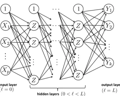
Artificial Neural Networks [9] are a computing model introduced in 1943, inspired by the structure of the biological neural networks that constitute our brain. A neural network is composed by a number of neurons (simple nodes that perform basic computations) that are connected to each other. In a more formal way, a neural network can be described as a directed graph whose nodes correspond to neurons and edges (also called arcs) correspond to links between them. Each neuron receives as input a weighted sum of the outputs of the neurons connected to its incoming edges. There are several types of neural networks, but we are interested in feedforward networks (in which the graph does not contain cycles). Usually we organise the network in layers: each layer contains a certain number of neurons and the inputs of the neurons at layer l+ 1 are the outputs of layer l. Each layer has also a constant node and the weight of the arc that connects this node to the nodes of the successive layer is called bias, while the weights of the arcs that connect the other non-constant nodes to the nodes of the successive layer are simply calledweights. Figure 2.1 shows a graphical representation of a neural network.

The first layer is called theinput layer and the neurons in this layer don’t have any incoming edges (in this case the neurons contain the values that are given as

Figure 2.1: An example of feedforward neural network with L+ 1 layers. Image taken from the material for Machine Learning course, DEI, Univ. of Padova (Prof. F. Vandin, 2017-2018).

input to the network); the last is theoutput layer and all the layers in between are calledhidden layers. The data flows from the input to the output layer. If we call

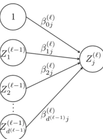
β_ij(l) the weight of the arc from node Z_i(l−1) of layer l−1to node Z_j(l) of layer l and we indicate the number of nodes at layerl asd(l)_{+ 1(see Figure 2.2 for a graphical} representation), then we can write the output of a generic node as:

Z_j(l)=θ  β (l) 0j + d(l−1) X i=1 β_ij(l)Z_i(l−1)  

whereθindicates a nonlinear transformation (usually a sigmoid, like the logistic function or the hyperbolic tangent).

When we are training neural networks we want to determine the values of the β_ij(l) for all the i, j, l such that the value of a certain cost (or loss) function is minimized (this is a standard procedure in most machine learning algorithms). The cost function compares the output of the neural network for a given input with the ground truth associated to that input and returns a value that grows with the prediction errors made by the network. To minimize this function we use a Gradient Descent algorithm (for example Stochastic Gradient Descent) and to calculate the gradient in an efficient way we use the Backpropagation algorithm. This second algorithm works in a two phase cycle:

• Propagation phase: the input is propagated forward through the network until it reaches the output layer. The output is then compared with the ground truth using the cost function. The resulting error value is calculated for each of the neurons in the output layer. The error values are then prop-agated from the output back through the network, until each neuron has an associated error value that reflects its contribution to the original output.

Figure 2.2: The point of view of one node Z_j(l). Image taken from the material for Machine Learning course, DEI, Univ. of Padova (Prof. F. Vandin, 2017-2018).

• Weight Update phase: the errors obtained with the previous phase are used to calculate the gradient of the loss function. The gradient is then fed to an optimization method that updates the weights, in order to minimize the cost function.

A very important parameter is thelearning rate, which determines how much the weights are updated at each iteration (it is a scalar that multiplies the quantity that updates the weight). Intuitively a small learning rate means that each iteration causes a “small” variation of the weights of the network, and so this could allow the network to consider the contribution of all the training examples and reach a good minimum point of the loss function, or it could just be too small and leave the loss function distant from a minimum. On the other hand, a high learning rate means the network updates the weights in a more ostensible way which could bring to faster convergence of the loss function or it could make the network give importance only to the more recent examples (since each iteration makes “big” changes to the weights), bringing the loss function away from a good minimum. Setting the learning rate to the right value is not easy and there are no formal rules; the choice has to be made by trying different values.

Sometimes, specially when the networks are big, the training examples have to be used more than once, since the update of the weights done by the backpropa-gation algorithm is usually small. A pass through the entire training set is called anepoch, and sometimes networks are trained for several epochs in order to reach the final weights for the model (usually the final model is the one that gives the best performance on the test set).

2.2

Adam Optimizer

As we saw in the previous section, the learning rate is a fundamental parameter for the training of a Deep Learning network, but it also difficult to find the “perfect” value. To alleviate the problem of finding the right learning rate, several optimiza-tion algorithms have been proposed and one of the most used (at the moment of

the writing it is almost considered standard) is the Adam Optimizer [10]. Adam is an optimization algorithm that can be used to update the network weights based on the training data, just as any other stochastic gradient descent algorithm. The difference is that it changes the learning rate over time, and in particular, the rate is adapted based on the average first moment (the mean) and the average of the second moment of the gradients (the uncentered variance).

The algorithm has 3 main parameters: α(the learning rate),β1 (the exponential decay rate for the first moment estimates), β2 (the exponential decay rate for the second-moment estimates). There is also a fourth parameter which is used to avoid a divide by zero error while updating the variable when the gradient is almost zero, and is usually set to be very small (e.g. 10−8). If we let f(θ) be an objective function that is differentiable with respect to the parametersθ(vector of parameters), then we can write the pseudocode for the Adam algorithm as follows (all operations on vectors are element-wise).

m0 ←0 (Initialize 1st moment vector)

v0 ←0 (Initialize 2nd moment vector)

t←0 (Initialize timestep)

while θt not converged do

t←t+ 1

gt← ∇θft(θt−1) (Get gradients w.r.t. stochastic objective at timestep t)

mt ←β1·mt−1+ (1−β1)·gt (Update biased first moment estimate)

vt←β2·vt−1+ (1−β2)·gt2 (Update biased second raw moment estimate)

ˆ

mt ← ₍₁m_−βtt

1) (Compute bias-corrected first moment estimate)

ˆ

vt← ₍₁₋vt_βt

2) (Compute bias-corrected second raw moment estimate) θt←θt−1−α· ₍√m_vˆˆt

t+) (Update parameters)

end return θt

In the original paper [10] there is also a theoretical analysis of the effectiveness of the algorithm and there is the pseudocode for a more efficient (but less clear) implementation, in addition to several empirical results that prove the qualities of the optimizer.

2.3

Convolutional Neural Networks

Convolutional Neural Networks (usually abbreviated as CNNs) are a class of feed-forward artificial neural networks. They are used for processing data that can be represented with a grid-like topology. In fact, the grid topology introduces a notion of “distance” or “correlation” among points and CNNs, as we will see, with their structure are able to exploit this information. Classic examples are images, which can be represented as a matrix of pixels, and time series data, which can be stored as a one dimensional vector with each element representing a sample at a given time. Like traditional neural networks, they are composed by an input layer, an output layer, and several hidden layers in between. The name “convolutional”

comes from the fact that particular layers of the network, known as convolutional layers, execute an operation calledconvolution on the data. In the next paragraphs we will see how convolutional layers work and what are the parameters that define them. We will then analyze the properties of CNNs and finally we will see other types of layers that can be found in a CNN architecture.

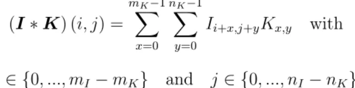
The convolution operation, which is different from a real mathematical convo-lution, takes two arguments: theinput and thekernel (sometimes it is also referred to as filter or neuron). In machine learning applications, the input is usually a multidimensional array of data and thekernel is a multidimensional array of learn-able parameters. If we have a two dimensional input I, with size mI ×nI, and a two dimensional kernel K, with size mK ×nK, we can define the convolution (denoted with the symbol∗) as:

(I∗K) (i, j) = mK−1 X x=0 nK−1 X y=0

Ii+x,j+yKx,y with

i∈ {0, ..., mI−mK} and j ∈ {0, ..., nI−nK}

As we can see from the definition, the convolution is basically a linear combination between the input and the kernel. We can also notice that the output of the operation is a matrix with size (mI −mK + 1)×(ni−nK + 1), which is smaller than the input. Figure 2.3 shows an example of convolution in a graphical format. The dimension of the kernel is called receptive field and the intuition behind this is that it corresponds to the portion of the input that the kernel “sees”. In this first example we used a stride of 1, which means that we are moving the filter of one position, after each convolution, but it is possible to set the stride to higher values. Stride values must be chosen carefully, in order to make sure that receptive field of the kernel fits correctly across the input. If we defines1 as the “row-stride” and s2 as the “column-stride”, the equation for the convolution becomes:

(I∗K)(i, j) = mK−1 X x=0 nK−1 X y=0

Is1·i+x,s2·j+yKx,y with

i∈ 0, ...,(mI−mK) s1 and j ∈ 0, ...,(nI−nK) s2

Figure 2.4 provides a graphical intuition of the effects of the stride value. We can immediately notice that stride affects the size of the output. In particular, the bigger the stride, the smaller the size of the output. This may be a problem: if we have an architecture composed of several convolutional layers, then the output size may decrease faster than we would like. A strategy used to control the size of the output volume is to pad the input with zeros around the borders. This technique is called padding and it is usually used to obtain an output with the same size of the input.

We can now define a convolutional layer as a layer where we convolve a certain number of kernels with the input to produce the output. The parameters we have to set are the number of kernels, their dimension, the stride used for each kernel and the presence or absence of padding. The parameters we want to learn are the

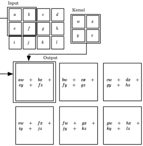
Figure 2.3: An example of 2D convolution: weconvolve the kernel with subsequent portions of the input. We start at the top left corner, execute a linear combination, and then move to the right by one position. Once we arrive to the right end of the matrix we return to the beginning and we move down of one position. Notice that the output is a 2×3 matrix, this is because there are 6 different locations that a

2×2 matrix can fit in the input. Image from [1].

Figure 2.4: Illustration of the effects of the stride value. The kernel is the vector

(1,0,−1) and the grey cells at the bottom are the input. On the left we have a stride of 1, while on the right we have a stride of 2. Image from [11].

values of the kernels.

Convolution provides a mean for working with inputs of variable sizes, and has three important attributes:

Sparse interactions In traditional neural networks, each output unit interacts with every input unit and we have a parameter for each interaction. In CNNs instead, we have sparse interactions because the kernel (which is usu-ally smaller than the input) interacts with a small portion of the input. We then have less parameters to store and computing the output requires fewer operations.

Parameter sharing Parameter sharing means using the same parameters for more than one function in the model. In a CNN, we saw that each ker-nel is convoluted in all the “fitting” locations of the input. This means that we are not learning a set of parameters for each location, we are only learning one set for all locations. Considering that the size of the kernel is usually sev-eral orders of magnitude smaller than the size of the input, parameter sharing allows us to dramatically improve efficiency in terms of memory requirements.

Equivariant representation The property of equivariance means that if the in-put changes, the outin-put changes in the same way. In CNNs we have that applying a transformation (for example a shift) to the input and then apply-ing convolution is the same as applyapply-ing convolution to the input (without transformation) and then applying the transformation.

Until now we treated the input as a matrix, but in practical applications we usually have a tensor as input. In mathematics a tensor can be defined in many ways, we propose here theintrinsic definition: letV be a vector space of dimension

n over a field _K and let V∗ be its dual. A tensor T of type (m, n) is then a multilinear application T :V × · · · ×V | {z } mtimes ×V∗× · · · ×V∗ | {z } ntimes →_K

A tensor can then be considered as an application that associates a scalar to m

vectors andn covectors.

In computer science we can consider a tensor as a multi-dimensional array. For example in pictures we have that each pixel is composed by three components (one for each RGB channel), and so the input is actually a tensor with the height and width of the image and depth equal to 3. Everything we saw in this section can easily be generalized to work with tensors, with only one additional detail: every kernel extends through the full depth of the input.

In real world applications we have multiple convolutional layers, one after an-other, and in each layer we have several kernels. Previously we saw that a con-volution is simply a linear combination, so, if we only used concon-volutional layers,

we would obtain a linear model, which may be too rigid to properly fit the data. For this reason, between different convolutional layers, it is common practice to include an activation layer. Activation layers apply a non-linear function to each component of their input and give the result as output. Several functions have been proposed over time, but we will focus on the Rectifier Linear Unit (usually abbreviated with ReLu). A paper by Krizhevsky et al. [12], has shown the effec-tiveness of this function and since then it became the “default” activation function for deep learning architectures (at the moment of the writing). ReLu is defined as:

ReLu(x) = max{0, x}

Some of the reasons of its popularity are the fact that it is very efficient, in the sense that it is easy to compute (and to implement), and the fact that its derivative is either zero or one (except in the point zero, where it is not defined). The latter is a desirable property because it reduces the likelihood of vanishing gradient and it simplifies the back-propagation steps. The vanishing gradient problem occurs when the gradient used to update the weights becomes too small, effectively preventing the weight from changing its value. However, it is important to say that there is no actual mathematical proof showing that ReLu is the best choice for the activation layer, we are basing our choices on empirical results.

To obtain the final prediction (a classification of the input) from a CNN (or in general a deep learning) architecture, it is common practice to put afully connected

layer as final layer. This layer is exactly like a layer of a traditional neural network and, for classification tasks, it is usually set to have a number of units which is equal to number of possible predictions. From the values contained in this final layer we can obtain the predicted label by looking for the unit with the highest value, or instead we can apply the softmax function and obtain the probabilities that the given input belongs to each different class.

Thesoftmax function (also known asnormalized exponential function) squashes an-dimensional vectorv of real values to an-dimensional vectors(v) of real values between 0 and 1 (extremes included). The function is defined as:

s(_jv) = e

vj

Pn−1

i=0 evi

for j = 0, ..., n−1

The value returned for i-th element of the output can be interpreted as the prob-ability that the input belongs to thei-th class.

There are also other types of layers that you can find inside CNN architectures (like pooling layers or network-in-network layers, just to cite a few), but we will not discuss them as, they are not needed for the DeepSense framework.

We conclude this section by saying that the kernels of the convolutional neural network can be learnt from the training data by defining a loss function and using theback-propagationalgorithm andstochastic gradient descent (usually, mini-batch stochastic gradient descent is used) or any other gradient descent method, as for traditional neural networks.

2.4

Recurrent Neural Networks

Recurrent neural networks (RNNs) are a class of artificial neural networks where the connections between units form a directed cycle and they are used for processing sequential data. Traditional neural networks do not have “memory”, in fact, for each new input, there is no information about previous results. This is a major shortcoming for tasks that involve sequential data, and RNNs were created exactly to solve this problem. The idea behind recurrent neural networks is to introduce cycles inside of the network, allowing information to persist. These cycles represent the influence of the present value of a variable, on its own value at a future time step. Loops inside of RNNs can be unfolded, composing a repetitive sequence of neural networks (Figure 2.5 illustrates this concept). In fact, the architecture of RNNs can be seen as amodule that is repeated for every time step.

Figure 2.5: RNNs can be unfolded into a chain of traditional neural networks. Many different recursive architectures have been proposed over time. We will focus onGated RNNs, and in particular on theLong Short-Term Memory (LSTM) model, introduced in 1997 by Hochreiter and Schmidhuber [13]. This model, as of this writing, is in fact the most used in practical applications like speech recogni-tion, handwriting generation and recognirecogni-tion, and parsing.

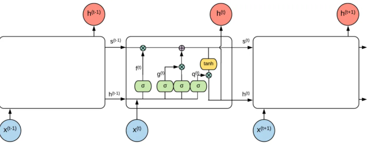
The repeating modules of an LSTM structure are called LSTM blocks. Each block can be thought of as a memory cell: it has a state, representing its stored value and it has an input gate, an output gate and a forget gate. This gates are regular artificial neuron units and, based on the value of their activation function, they “open” or “close” the gates, letting the input flow or blocking it. Figure 2.6 shows a graphical representation of a LSTM block. From the figure we can notice several things:

• an input can be accumulated into the state if the input gate allows it.

• the state has a linear self-loop whose weight is controlled by the forget gate.

• the output of the cell can be shut off by the output gate.

Figure 2.6: Diagram of an LSTM block. The black square indicates a delay of a single time step. An unfolded version of the architecture can be seen in Figure 2.7. Image from [1].

If we consider the input as a vector, each LSTM block receives the whole vector as input. For this reason we usually have multiple blocks (also called cells), that can be interpreted as a memory system, were each cell takes care of saving specific information (or features) about the data. Before writing the forward propagation equations we need to define some elements:

• x(t) is the input vector at time step t

• h(t) _{is the hidden layer vector (containing the outputs the LSTM cells) at} time step t

• s(t)_i is the state unit of the i-th cell at time step t

• f_i(t) is the forget gate of the i-th cell at time step t

• g_i(t) is the external input gate of thei-th cell at time step t

• q_i(t) is the output gate of the i-th cell at time step t

• b,U,W are the biases, input weights and recurrent weights into the LSTM cell

• bf_,Uf_,Wf _{are the biases, input weights and recurrent weights for the forget} gate

• bg_,Ug_,Wg _{are the biases, input weights and recurrent weights for the} exter-nal input gate

• bo,Uo,Wo are the biases, input weights and recurrent weights for the output gate

• with the symbolσ we indicate a sigmoid function with an output between 0 and 1 (extremes included)

We can now write the forward propagation equations as follows:

f_i(t) =σ bf_i +X j U_i,jf x(t)_j +X j W_i,jf h(t_j−1) ! (a) s_i(t) =f_i(t)s_i(t−1)+g_i(t)σ bi+ X j Ui,jx (t) j + X j Wi,jh (t−1) j ! (b) g_i(t) =σ bg_i +X j U_i,jg x(t)_j +X j W_i,jg h(t_j−1) ! (c) h(t)_i =q_i(t)tanh(s(t)_i ) (d) q_i(t) =σ bo_i +X j U_i,jo x(t)_j +X j W_i,jo h(t_j−1) ! (e) From equations (a), (c) and (b) we can see that all gates have the same structure, they only have different weights that define their behaviour. Equation (a), shows us that the input at time stept, and the output of the previous cell (h(t−1)_{) influence} how much of the state we want to forget. From equation (b) we can understand how the LSTM cells updates work. In particular, in equation (b), we have that the previous state (s(t−1)_{) is multiplied by the forget gate and then added to the} product of the external input gate g_i(t) and the candidate values that could be added to the state. It’s like if equation (a) decides what we want to forget and equation (c) decides how much we want to update the state. After deciding what to forget and how much to update we have equation (b), which actually forgets what has to be forgotten and adds the new information. In equation (d) we can see that the cell state is passed through tanh, to obtain a value between -1 and 1 and then it is multiplied by the output gate q(t)_i , that decides how much of the output we want to pass.

A successful variant of LSTM, that has recently been proposed, is the gated recurrent unit model (abbreviated with GRU [14]). The main difference with the LSTM structure is that a single gating unit simultaneously controls the forgetting factor and the decision to update the state unit. In GRUs there is also no output gate, so the final model is significantly “lighter” than LSTM, but it seems to give very good results in practical applications. The update equation for GRUs is:

h(t)_i =u(t_i−1)h_i(t−1)+ (1−u(t_i−1))σ bi+ X j Ui,jx(t)j + X j Wi,jr(t −1) j h (t−1) j ! (f)

Figure 2.7: An unrolled representation of a LSTM structure showing the repeating module.

where u stands for “update” gate and r for “reset” gate and their value is defined as the other gates we saw previously:

u(t)_i =σ bu_i +X j U_i,ju x(t)_j +X j W_i,juh(t_j−1) ! r_i(t) =σ br_i +X j U_i,jr x(t)_j +X j W_i,jr h(t_j−1) !

From equation (f) we can see that update and reset gates can individually ignore part of the state vector, removing the need of separate gates.

2.5

Dropout

With deep learning architectures there is always a high risk of overfitting. Overfit-ting occurs when a model doesn’t capture the underlying structure of the data, but only adapts to the training data. This means that the model becomes extremely good at predicting the data that has it has been trained on, but isn’t then able to generalize and performs poorly on unseen data. A common practice that is used to tackle this problem is called dropout [15]. This technique is applied only dur-ing the traindur-ing phase and it consists in randomly droppdur-ing units from the neural network. In practice, this means that we randomly set to zero a certain amount of activations in a layer. This amount is controlled by setting the probability of dropout (usually 0.5 is used).

In a more formal way, if we define z(l) as the vector of the inputs into layer

l, y(l) _{as the outputs of layer l, W}(l) _{and b}(l) _{as the weights and biases al layer}

l and f as an activation function, then the feed-forward operation with dropout becomes:

˜

y(l) =r(l)∗y(l)

z_i(l+1) =w_i(l+1)y˜(l)+b(l+1)_i y_i(l+1) =f(z_i(l+1))

where ∗ indicates an element-wise product and y˜(l) _{is the output of layer l with} dropout. The parameter p of the Bernoulli random variable is the probability of dropout that we can set. Figure 2.8 shows the graphical representation of a node in a neural network when dropout is applied. The training of a dropout network is still

Figure 2.8: Dropout network. Image from [15].

done with a gradient descent technique and the Backpropagation algorithm. The only difference is that for each training example we consider a “thinned” network by dropping out units (forward and backpropagation for the training example are done only on the thinned network). When we have finished training and we want to use the network to predict the output for a given input, we don’t apply dropout (in a certain sense it can be seen like if we setp= 1). Several empirical results have shown the effectiveness of dropout and it is a common procedure for the training of Deep Learning architectures.

2.6

L2 Regularization

In the previous section we already talked about the problem of overfitting and how dropout can help, but there are also other ways to avoid (or at least reduce) overfitting, and regularization is one of them. Regularization consists in adding a penalty term to the loss function as the model complexity increases. In L2 regularization, also known asridge regression, the penalty term is defined as:

λX

i

Where βi are the weights of the model and λ is a parameter that defines how much “importance” we are giving to the regularization (if it is equal to zero, then there is no penalty, if it is large then it may add too much penalty and lead to under-fitting). Intuitively the idea behind regularization is that we want to force the weights to be as simple as possible, and this should make them more “general” and less “specific” for the training examples.

2.7

Batch Normalization

When working with famous datasets available online, we usually have the training data and the test data coming from the same distribution. However, in real world problems, this happens very rarely. When the data from training and testing comes from different distribution we are experiencing a dataset shift. There are several types of dataset shifts, but the only one we can actually mitigate iscovariate shift. Covariate shift refers to the change in the distribution of the input variables present in the training and the test data. In neural networks, covariate shift,

ap-Figure 2.9: Graphical example of covariate shift. Image from [16].

pears also between different layers of the network, and it is calledinternal covariate shift. This happens because a change in the parameters of a layer affects all the successive layers, and even small changes can have big effects on deeper layers. These shifts in the distribution of each layers input, make it hard to train the net-work and require careful parameter initialization and lower training rates (things that considerably slow down the training process). A paper by Ioffe and Szegedy [17] proposes a technique called batch normalization that is able to alleviate this problem and that allows us to to use higher learning rates and be less careful about initialization. Previous studies [18] have shown that, if the inputs of a NN are transformed to have zero mean and unit variance, the speed of training can be increased. Batch normalization follows this idea and works by fixing the mean and the variance of the inputs of each layer in an efficient way. Simply normalizing each input of a layer may change what the layer can represent, so there are also a pair of parameters (for each activation),γ and β, which scale and shift the normalized values. These parameters are learned during training.

We can now see how the batch normalization process works. Since the nor-malization is applied to each activation independently, we will focus only on one particular activation of a certain layer. Let _B = {x1, x2, ..., xm} be the set con-taining the values of the activation, over a mini-batch of m inputs. With xˆ1,...,m we refer to the normalized values, whiley1,...,m are their linear transformation. We can now define the algorithm for batch normalization as follows:

1. µ_B ← 1 m

Pm

i=1xi (mini-batch mean) 2. σ2 B← 1 m Pm i=1(xi−µB) 2 _{(mini-batch variance)} 3. xˆi ← √xi−µB σ2 B+ (normalization)

4. yi ←γxˆi+β (scaling and shifting)

The finaly values are passed as input to the next layer. The that can be found at step 4 is a scalar (usually set to be very small), used to avoid a division by zero. A compact way of defining the normalization for a generic vector h is:

BN(h;γ,β) = β+γ∗_ph−E[h] Var[h] +

Where the division is intended as component-wise. Batch normalization transform is a differentiable transformation and so the network can still be trained using gradient descent (or any of its variants) and the back-propagation algorithm.

There is also a version for recurrent neural networks that is called Recurrent Batch Normalization [19]. In this case batch normalization is introduced in the input-to-hidden and the hidden-to-hidden transformations. For example the equa-tions for LSTM that we saw in chapter 2.4 become:

f(t) =BNUfx(t);γ_Uf,β_Uf+BNWfh(t−1);γ_Wf ,β_Wf +bf

g(t)=BN Ugx(t);γ_Ug,β_Ug+BN Wgh(t−1);γ_Wg ,β_Wg +bg

q(t) =BN Uox(t);γ_Uo,β_Uo+BN Woh(t−1);γ_Wo ,β_Wo +bo

s(t) =f(t)∗s(t−1)+U x(t)+W h(t−1)+b h(t) =q(t)∗tanh BN s(t)

Where∗stands for the component-wise product. One particular observation is that the β parameters of the normalization are set to zero, because there are already the b vectors that account for bias.

Batch normalization has proven to be very effective and, at the moment of the writing, it is considered a standard procedure for deep learning architectures.

Chapter 3

DeepSense Architecture

The paper by Yao et al. [2] describes the structure of the DeepSense framework (Figure 3.1). However, the authors do not enter into the details of the parameters of the architecture. In fact, elements like the dimensions of the CNN filters, the stride, the eventual padding added to the input, the number of units of the GRU layers and the size of the fully connected layers are not specified. Unfortunately, we do not have access to the source code that has actually been used for the work described in the paper, but one of the authors released a Python implementation of the DeepSense framework on github2_{, together with an already pre-processed} dataset3 _{and the code used for the pre-processing. From the code available on} github we can obtain the parameters that are missing in the article but we do not have the certainty that we will be recreating the exact framework that the authors implemented for their tests. We will see this as an opportunity to play with the different parameters and to test which values give us the best results.

In the next sections we will illustrate the DeepSense framework and we will ex-plicitly specify the differences between the Python implementation available online and the architecture described in the paper. For each section we will present the framework with a general notation (as in the paper), together with a more practical point of view, by specifying the exact values for all the necessary parameters.

We will start by describing how the data obtained from the sensors is repre-sented in theory. Let k be the number of available sensors (in our case k = 2, as we have data from the accelerometer and from the gyroscope), and let _S = {Si} be the set containing all the sensors Si, with i∈ {1, ..., k}. For each sensor Si we will store its measurements with a matrix V and a vector u:

• V has size d(i)_×n(i)_{, where d}(i) _{is the number of dimensions for each} mea-surement (in our case it is equal to3 for both accelerometer and gyroscope) and n(i) is the number of measurements.

• u has sizen(i)_{, and contains the timestamp of each measurement.}

In other words, for every different sensor, we are considering each measurement as a column vector (with one component for each measured dimension) and we are stacking them, one after another, as we collect them from the sensor, composing

2

https://github.com/yscacaca/DeepSense

3

a matrix. As we will see, in the implementation we will not have the vector u

of timestamps because we will interpolate the data and take a certain number of uniformly distributed “measurements” from the function obtained with the interpo-lation. Notice that if we wouldn’t perform this process of interpolation, the vector

uof timestamps would be necessary, because otherwise, we would lose the relation in time of the different measurements (real sensors almost never take measurements at a fixed rate and at fixed time intervals).

3.1

Data Pre-Processing

We will now propose the pre-processing as it presented in the paper, and then we will see how it is actually done with the data from the HHAR dataset and what problems we can encounter.

In theory

For each sensorSi, i∈ {1, ..., k}:

• Split the input measurements V(i) _{and u}(i) _{along time to generate a series} of non-overlapping intervals with width τ. Store this intervals in the set

W(i)={(Vt(i),u (i)

t )}, where |W(i)|=T and t∈1, ..., T.

• For each pair inside of_W(i) _{apply the Fourier transform and stack the inputs} into a d(i)_{×2f ×T tensor X}(i)_{, where f is the dimension of the frequency} domain containingf magnitude and phase pairs.

Finally, group all the tensors in the set _X = {X(i)_{}, i∈ 1, ..., k, which is then the} input of the DeepSense framework.

On the HHAR Dataset

In the code available online, the authors pre-processed the HHAR dataset and saved it in a series of.csv files. This files will then be the input for their implementation of DeepSense (in this way it is not necessary to perform the pre-processing each time). We will now describe the process they used to obtain the .csv files. For each of the 6 activities in the HHAR dataset:

• Collect all the raw measurements for the activity.

• Segment the raw measurement in 5 seconds samples.

• Divide each sample into time intervals of lengthτ = 0.25 seconds (this divi-sion gives usT = 20).

• Interpolate the measurements of each time interval of lengthτ = 0.25.

• Take 10 uniformly distributed “measurements” from the resulting interpolated function of each interval and apply the Fourier Transform to each of them. Each measurement is a vector of length 3 of real values, so we have that

the the FFT function will return a complex-valued vector of length 3. This complex values are divided into real part and imaginary part pairs and this gives us 6 real values for each measurement. In their code, the authors call these pairs Spectral Samples. Notice that in the theoretical procedure we took magnitude and phase, while here we are taking of real and imaginary part (the results are the same, it is only necessary to choose a representation and be consistent).

• Save the 10 spectral samples for each of the 20 intervals that compose the 5 second sample in a .csv file, for a total of 20×10×6 = 1200 real values per sample. In the file, after all the spectral samples values, there is also the one-hot encoding of the ground truth (inside each.csv file there are 1206 values).

In the DeepSense code provided by the authors, the framework is implemented using the TensorFlow library [20]. TensorFlow has some specific requirements for how the data has to be represented. For this reason we will see that the practical implementation of the framework is very different from what the authors propose in the paper.

When we need to use the data, we will read the values from the .csv files and, for each 5 second sample, we will store them into two matrices (one for each sensor) of size20×60 (we basically have one row for each time interval of length

τ containing 6 real values for each of the 10 spectral samples).

In real world scenarios, sensors do not guarantee fixed sample rates, so if we collect data for a certain amount of time, we might have a different number n(i)

of measurements for each sensorSi. To deal with this problem, the authors make sure that each 5 seconds sample is composed by 20 intervals of lengthτ, by adding some all zero intervals at the end (if necessary). Successively, as we will see, they take into account of this “fake” intervals in the RNNs layer and in the output layer. The authors also used somedata augmentation on the dataset to make it more robust (it was not written in the article but it can be found in the code). In par-ticular for each training example they added other 9 examples obtained by adding noise (with a random normal distribution with zero mean and0.5variance for the accelerometer and 0.2 variance for the gyroscope). Referring to the procedure we described for the pre-processing the augmentation would be made at the second step, where from each 5 seconds sample we would generate other samples. The reasoning behind this is that the data generated by the sensor is already noisy, and so having more samples with slightly different noise should make the network more robust to it.

3.2

CNN Layers

The convolutional neural network layers of the DeepSense architecture can be di-vided in two parts: Individual Layers and Merge Layers. The first part keeps the data from different sensors separated, while the second part merges the data from the two sensors.

3.2.1

Individual Layers

On the theoretical side, for each sensorSi and for each time interval t, the matrix

X(i)_:,:,t is fed into the architecture. On the practical side, the input of the architecture is composed by a matrix of size20×60, for each 5 seconds sample (as we specified in the pre-processing section). For simplicity, from now on, we will denote the stride with a tuple, where the i-th element indicates the stride value for the i-th dimension. For example, if we have a two-dimensional input, and we want to move the kernel of 1 position on the first dimension and of 3 positions on the second dimension, we have a stride of(1,3).

1. The first CNN individual layer applies 64 2D filters with shape d(i)_×cov1, producingX(i,1)_:,:,t as output.

In the article the value of cov1 is not specified, but from the Python imple-mentation of DeepSense we obtained that each filter covers 3 samples and has a stride of 1 sample. In detail this means a filter of size1×(6∗3)and a stride of(1,6).

Right after this layer we apply batch normalization, then we apply a ReLu activation layer and finally we apply dropout with probability0.8of keeping the connections to the next layer (this probability was not specified in the paper, but we obtained it from the Python implementation).

2. The second layer applies 64 1D filters with shape 1×cov2, producingX(i,2)_:,:,t

as output.

The size of this filters are, again, not specified in the paper but from the code we found that it is (1,3) with stride (1,1).

We then perform batch normalization, add a ReLu activation layer and per-form dropout as before.

3. The third layer applies 64 1D filters with shape 1×cov3, producingX(i,3)_:,:,t as output.

The size and stride of the filters are the same of the previous layer.

Finally we apply batch normalization and pass the results through a ReLu activation layer.

The intuition behind the first CNN layer is that we want to extract relationships, within the frequency domain, across sensor measurement dimensions and look for local patterns in neighbouring frequencies. For the second and third convolutional layers, it is difficult to find a precise intuition, but we can say that they are learning high-level relationships.

Finally, at the end of the individual layers, we flatten the matrix X(i,3)_:,:,t into a vector x(i,3)_:,:,t and concatenate all k vectors into a k-row matrix X(3)_:,:,t which is the input of the merge convolutional subnet. To understand how the concatenation is done in the implementation of DeepSense provided by the authors, we first need to look at the size of the output of each convolutional layer (batch normalization layers, ReLu layers and dropouts leave the size unchanged).

• At the first layer, the stride and the size of the kernels give us an output of size 20×8 (for each of the 64 kernels applied).

• At the second layer we obtain an output of size 20×6 (for each of the 64 kernels applied).

• At the third layer we finally have an output of size20×4(for each of the 64 kernels applied).

• The final20×4matrices are reshaped to obtain a20×1×4tensor (basically we are just adding a dimension).

So at the end, for each kernel of the third layer, we have a20×1×4tensor. Remem-ber that this is done for each sensor, so we will have one tensor (for each kernel) for the accelerometer and another for the gyroscope. These two are concatenated in a20×2×4 tensor, that is the input of the Merge Layers. This concatenation process may seem strange, but it is necessary for how the TensorFlow framework works (we will enter in more details about TensorFlow in Chapter 5).

3.2.2

Merge Layers

The merge convolutional subnet is very similar to the individual convolutional subnet in it’s structure, but from the code we can see that there are some important differences in some of the parameters.

1. We first apply 64 2D filters with shape k×cov4 (here the intuition is that we want to learn the interactions among allk sensors) with outputX(4)_:,:,t. As we did before, we apply batch normalization, a ReLu activation layer and dropout with probability0.8of keeping the connections.

From the code we found that the size of the filters is 1× 2×8 and the stride is of(1,1,1). We also found that padding is applied in order to obtain an output of the same size of the input. Notice that without padding it wouldn’t be possible to have a kernel of the given size, because the input is of size 20×2×4.

2. We then apply 64 1D filters with shape 1×cov5, and output X(5)_:,:,t.

The size of the filters is 1×2×6 and the stride is of (1,1,1). Padding is applied as before.

Like in the previous layer, we apply batch normalization, then a ReLu activa-tion layer and finally dropout with probability0.8of keeping the connections. 3. Finally we apply 64 1D filters with shape 1×cov6, and outputX(6)_:,:,t.

The size of the filters is1×2×4 and the stride is of(1,1,1). Again, in this layer, padding is applied.

At the end of this layer batch normalization and a ReLu activation layer are applied.

We then flatten the final output X(6)_:,:,t into vector x(f)_:,:,t; concatenate x(f)_:,:,t with time interval widthτ, and obtain the vector x(c)_t . The vectorsx(c)_t fort∈1, ..., T are the

input of the RNN layers. As for the individual layers, the concatenation done in the Python implementation of DeepSense is different from what we have in theory. In particular it is done by transforming each 20×2×4tensor in a 20×8matrix. From the code we also noticed that the time interval width τ is not concatenated to the output, differently from the theoretical procedure.

3.3

RNN Layers

The recurrent neural network layers of the architecture are relatively simple. In fact we have 2 GRU layers stacked one on top of the other. We apply dropout to the connections between the two layers and we use Recurrent Batch Normalization [19]. The output of the GRU layers is the set of vectors {x(r)_t } for t∈1, ..., T.

In the GRU layers provided by TensorFlow it is possible to set the length of the sequence of each sample. In this way we can take care of the problem of different sequence lengths that appears in real world scenarios. The fact that TensorFlow offers the possibility to specify the length of each sequence is probably the reason why they didn’t concatenate the time intervalτ at the end of the merge layers.

In the paper the authors do not specify the number of units in the two GRU layers and they do not specify the probability of keeping a connection in dropout. From the code on github we can see that the probability of keeping a connection in dropout is 0.5and that the number of units in the GRU layers is 120 for both.

120is exactly the number of “features” for time interval. In fact we previously saw that for each interval of length τ we have 10 spectral samples (each composed of 6 real values). Given that we have two sensors, there are exactly 10×6×2 = 120

values to represent each interval of length τ. We can confirm that the number of units in the GRU layers is set to match the number of “features” that represent a time interval by the fact that the authors explicitly write thatx(r)_t is the “feature vector at time intervalt”.

In the Python implementation we obtain a 20×120 matrix as output for each 5 seconds sample.

3.4

Output Layer

In the output layer we want to obtain the final prediction of the activity recognized by the DeepSense framework. This is done by averaging the feature vectors x(r)_t

over all the time intervals of length τ, to obtain the final feature vector:

x(r) = PT t=1x (r) t T

We then feedx(r) _{into a softmax layer to obtain the predicted category probability} vector yˆ. In the Python implementation this is done by performing the average feature vector, as described, and then connecting it to a fully connected layer with 6 units (one for each activity). Finally softmax is applied to the output of this fully connected layer to obtain the probabilities of the different activities.

As we saw in the pre-processing section, in a real world scenario, not all the intervals have the same length T, so we will need to take into account the real length of each interval when calculating the final vector.

3.5

Loss Function and Regularization

The loss function chosen by the authors isCross Entropy. The Cross Entropy loss function is defined as:

L=− 1 |Training Set| X x∈Training Set M X c=1 yx,clogpx,c

WhereM is the number of classes (6 in our case), xis a training example,yx,c is a binary indicator (0 or 1) if class label cis the correct classification for observation

x, and px,c is the predicted probability observation x is of class c. Cross Entropy can be considered as the default loss function for multiclass classification tasks. It wasn’t written in the paper, but from the code available on github we saw that the authors applied L2 Regularization, withλ = 0.0005.

Chapter 4

Customizing DeepSense

The authors of DeepSense wanted to create a “general” Deep Learning model to work with time-series data coming from sensors, so they didn’t worry about pushing the performances for a specific task. In fact, the framework proposed by the authors, is meant to be trained only once and then to be deployed on device “as-is”. Differently, we are focusing only on human activity recognition and we want to achieve the best possible result. One thing that comes to mind about the human activity recognition problem is that it is highly “personal”, in the sense that a single smartphone or smartwatch is used by just one person, and the style of walking, running or climbing stairs is peculiar to each individual. Our idea was then to exploit this characteristic of the problem by modifying the framework in order to make it able to adapt over time to a specific user, increasing the accuracy of its predictions. Talking with a high level of abstraction, we want to utilize the original framework trained on the HHAR dataset as a starting point for a more personalized system. In particular, in the first period of utilization by the user, we will predict the activity he is performing with the original framework, and then we will ask if the prediction is correct. Each feedback given by the user will successively be used to modify the system, making it more and more “personal”. Ideally, this will increase the accuracy of the model over time.

To implement this strategy in practice we used the concept oftransfer learning. Transfer learning is a machine learning method where a model developed for a task is reused as the starting point for a model on a second task. The typical scenario in a transfer learning setting is to have a base network already trained on a certain dataset, which is then repurposed as a part of a second network which is trained on the target dataset. In our case we will use the the DeepSense framework, from the input layer, to the GRU layers included, as our base model, and we will have a separate network representing the output layer as our target network that will be trained with the data generated by the user. In more detail we followed this procedure:

1. We selected a user and we splitted he’s original data into two halves, one for training, and the other for validation. The split was done at the activity level: for each activity we took half of the data for training and half for validation (this preserves the ratio of examples between the different activities).

all the users, except the data of the user chosen at step 1), and we extracted the values of the weights and bias of the output layer (which we remember is a fully connected layer that receives as input the average of the vectors given by the GRU layers).

3. We created a new network consisting only of a fully connected layer that receives as input a vector of length120and gives as output a vector of length

6consisting of the probabilities associated to each activity for the given input. 4. We initialized the second network with the weights and bias of the output

layer of the full DeepSense model that we trained in step 2.

5. We trained the second network with the training data of the specific user selected at step 1.

6. We evaluated the performance of the second model with the validation data of the specific user selected at step 1.

This procedure suggests a possible scenario where a user with a new device (or application) inserts feedback on the predictions, generated by the application that performs human activity recognition, for a certain number of times, in order to make the model adapt to himself. The application then stops asking for feedback and, from now on, generates new predictions using the adapted model. These pre-dictions should be more accurate than the ones given by the “general” DeepSense framework trained only on the HHAR dataset, since they are based on data ob-tained directly from the user. In the next Chapter we will see exactly the tests that have been done to evaluate the effectiveness of the transfer learning technique on the DeepSense framework and in Chapter 6 we will show the results we obtained. Before moving on to the tests section, we will spend a few words on how to actually implement this kind of transfer learning strategy on a device. First of all it is necessary to have a saved full DeepSense model trained on the HHAR dataset. This model will never be modified and it will only be used to generate predictions, and in particular to obtain the input to the output layer. Saving a model can easily be done with TensorFlow’ssavedModel format, as we will see in the next Chapter. Then we will need to have a second model consisting of a fully connected layer that will be trained with the feedback given by the user on the predictions. As previously mentioned in this section, we will initialize this model with the values of the weights and bias of the output layer of the full trained DeepSense model. The second model will then require some training steps, and usually you would not want to perform training on a smartphone or smartwatch, but in this case we have a simple fully connected layer and it shouldn’t be a problem for modern devices in terms of time, computing resources and power consumption to perform this operation. We can then describe the prediction procedure as follows:

1. Collect the data form the sensors and execute the necessary pre-processing (see chapter 3.1).

2. Pass the data as input the the full DeepSense model and obtain the output of the GRU layers. We called this outputx(r) _{in chapter 3.4.}

3. Passx(r) _{to the second model consisting of a fully connected layer and obtain} the predicted activity.

4. Ask to the user if the prediction was correct.

5. Use the feedback given by the user to create a new training example that will be used to perform a training step on the second model.

Points 4 and 5 could be skipped after a certain number of times in order to not “disturb” the user requiring continuous feedback and to avoid overfitting.

Chapter 5

Experimental Tools & Settings

All the code generated for this thesis was written in Python with an extensive use of the TensorFlow library [20]. In particular the code requires Python 3.x,

TensorFlow 1.5.x or greater and the NumPy package4_{. The tests were ran on} a cluster composed of 40 IntelRXeon ES-2698 v3 cpus (each with 16 cores and 40960 Kb of L3 cache) and a total of 528 Gb of RAM. The code is organized in the following files:

• deepSense.pyThis file contains the implementation of the DeepSense frame-work.

• transferLearning.py This file contains the implementation of the custom model we created (explained in Chapter 4).

• test01.pyImplementation of Test 1 (see section 5.2)

• test02.pyImplementation of Test 2 (see section 5.2)

• test03.pyImplementation of Test 3 (see section 5.2)

• test_main.pyThis file contains a simple script that launches the tests.

• sepUsers.py This and the next files are the implementation of the pre-processing required for DeepSense (see Chapter 3.1). The code in this file creates one folder for each user, and inside each folder it creates two.csv files that will contain accelerometer and gyroscope data for that user.

• augmentation.py This file performs data augmentation, as described in Chapter 3.1.

• mergeSensors.pyThis file merges the measurements from accelerometer and gyroscope, doing all the necessary pre-processing, and organizing the data in

.csv files with the structure described in Chapter 3.1.

• prepareCV.py This file contains a script that organizes the data in folders for leave-one-out cross validation.

In the next sections of the chapter we will enter in more details about Tensor-Flow, and the tests that we performed.

4_{Available at}