Pareto Multi-Objective Non-Linear Regression
Modelling to Aid CAPM Analogous Forecasting.
Jonathan E. Fieldsend and Sameer Singh
PANN Research Group, Department of Computer Science,
University of Exeter, Exeter, EX4 4PT, UK
Abstract - Recent studies confront the problem of multiple er-ror terms through summation. However this implicitly assumes prior knowledge of the problem’s error surface. This study con-structs a population of Pareto optimal Neural Network regression models to describe a market generation process in relation to the forecasting of its risk and return.
I. INTRODUCTION
The use of Neural Networks (NNs) in the time series focasting domain is now well established, with a number of re-cent review and methodology studies (e.g. [1], [2], [3]). The main attribute which differentiates NN time series modelling from traditional econometric methods is their ability to gen-erate non-linear relationships between a vector of time series input variables and a dependent series, with little or no a
pri-ori knowledge of the form that this non-linearity should take.
This is opposed to the rigid structural form of most economet-ric time series forecasting methods (e.g. Auto-Regressive (AR) models, Exponential Smoothing models, (Generalised) Regressive Conditional Heteroskedasticity models, and Auto-Regressive Integrated Moving Average models) [4], [5], [6]. Apart from this important difference, the underlying approach to time series forecasting itself has remained relatively un-changed during its progression from explicit regression mod-elling to the non-linear generalisation approach of NNs. Both of these approaches are typically based on the concept that the most accurate forecast, if not the actual realised (target) value, is the one with the smallest Euclidean distance from the actual. When measuring financial predictor performance however, practitioners often use a whole range of different error sures (15 commonly used time series forecasting error mea-sures alone are reported in [7]). These error meamea-sures tend to reflect the preferences of potential end users of the fore-cast model. For instance, in the area of financial time series forecasting, correctly predicting the directional movement of a time series (for instance of a stock price or exchange rate) is arguably more important than just minimising the forecast Euclidean error.
In order to encapsulate multiple objectives, recent ap-proaches to time series forecasting using NNs have introduced augmentations to traditional learning algorithms. These have been in the form of propagating a linear sum of errors [8], [9], [10], and penalising particular mis-classifications more heavily [11].
However these approaches implicitly assume the
practi-tioner has some knowledge of the true Pareto error front de-fined by the generating process, and the features and network topology they are using to model it. A Pareto error front is defined such that a feasible model lying on the Pareto front cannot improve any error (by the adjustment of its parameters) without degrading its performance in respect to at least one of the others. Therefore, given the constraints of the model, no solutions exist beyond the true Pareto front.
Given that it is likely that the error surface defined by the generating process is not known, a new approach to imple-menting multiple objective training within NNs is needed.
Through the use of a Multi-Objective Evolutionary Algo-rithms (MOEAs) it is possible to find an estimated Pareto set of the combinations of parameters to multiple objective ‘clean’ function modelling problems [12], [13], [14]. Over the previous 15 years, since the work by Schaffer [15], MOEAs have been applied to a vast number of design problems, where mathematical formulae define the multiobjective surface to be searched. These methods had not, until very recently, been applied to the noisy domain of multi-objective neural net-work (MONN) generalisation. The first and, to the author’s knowledge, only study using a MOEA to train a population of MONNs is that by Kupinski and Anastasio [16]. In their study a population of MONNs are trained using the Niched Pareto Genetic Algorithm (NPGA) MOEA developed by Horn et al. [17], which are applied in the medical image classifica-tion domain, to a synthetic two-class problem. In this study however the methodology used in [16] is extended, by the use of a MOEA with proven superiority in the noiseless domain to the NPGA (the Strength Pareto Evolutionary Algorithm [18], SPEA) and applied to real data in the financial time-series fore-casting domain.
Once a set of MONNs, that lie upon the Pareto Surface in error space, have been generated, a practitioner gains knowl-edge with respect to the error interactions of their problem. In addition they also have the opportunity to select an individual model that encapsulates their error preferences, or a group of models if so desired. By analogy with the Capital Asset Pricing Model (CAPM) it is demonstrated that by generating a Pareto set of models with respect to estimated risk and return, the practitioner can access higher rates of return (for a given level of risk) by diversifying their wealth between forecast-based ar-bitrage and ‘risk-free’ investments.
This study takes the following form: a more formal overview of the current approach to multi-objective optimisation in the
forecasting domain is presented in Section II. Pareto optimal-ity is presented in Section III and the CAPM model is intro-duced in Section IV. This is followed in Section V by a brief description of the data used and the measures of risk and re-turn used in training. In Section VI experiments and results are discussed with conclusions and further work contained in Section VII.
II. CURRENT APPROACH
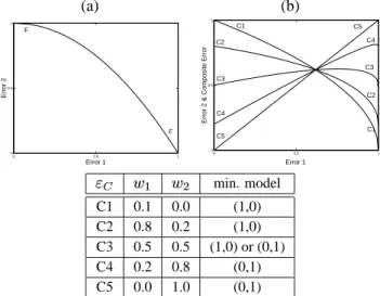
An illustration of the problems associated with the current approach to multi-objectivity in NN regression is provided in Figure 1(a) and 1(b).
(a)
(b)
Fig. 1. (a) Two-dimensional error surface 1. (b) Two-dimensional error surface 2.
Consider the situation where two error measures are used that lie in the range [0,1]. Given that the practitioner wishes to minimise errors, the typical approach in linear sum
back-propagation is to minimise the composite error
, in the D error measure case (where the errors are to be minimised) this is calculated as follows: ! (1) where"$#%'& & .
In the two dimensional case illustrated in Figures 1(a) and 1(b), where the practitioner gives equal weighting to both er-rors, and both errors lie within the same range, this is calculated
as: % )( % ( (2) This approach implicitly assumes that the interaction be-tween the two error terms is symmetric. Consider Figures 1(a) and 1(b): Figure 1(a) illustrates the situation described, where the minimum error surface defined by the problem is shown as the Pareto front FF. On its extremes it can be seen that the error combinations (0.0, 1.0) and (1.0, 0.0) are possible, which de-fine the axial symmetric hyper-boundaries of the front. In ap-plying eq. 2 the composite error curve CC is generated. As the illustration shows, if the training process of the model reaches the error front (the true Pareto front), the model returned will be at the minimum of the composite curve, and defined by (e1,e2). In the case of Figure 1(a), this model can be seen to have the error properties (0.50, 0.32). Figure 1(b) illustrates the same situation, with identical hyper-boundaries but a slightly
differ-ent degree of convexity of the front*+* . In this case the model
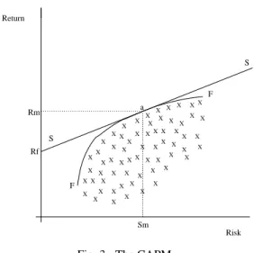
returned is defined by the error properties (0.42, 0.22). The two models are significantly different, and in both cases, due to the shape of the Pareto error fronts (and contrary to the desires of the user), the error properties of the models returned are not equal. Although the feasible range of both error measures are the same, the interaction of the errors, as demonstrated by the shape of their true Pareto fronts, results in the return of mod-els, that though Pareto optimal in themselves, do not represent the preferences of the practitioner. An even worse situation arises if the true Pareto front is concave and not convex. In this case composite error weighted summation will only return those models on the extremes of the Pareto front, as illustrated in Figure 2. (a) (b) 0 0.5 1 0 0.5 1 Error 1 Error 2 F F 0 0.5 1 0 0.5 1 Error 1
Error 2 & Composite Error
C1 C1 C2 C2 C3 C4 C5 C5 C4 C3 min. model C1 0.1 0.0 (1,0) C2 0.8 0.2 (1,0) C3 0.5 0.5 (1,0) or (0,1) C4 0.2 0.8 (0,1) C5 0.0 1.0 (0,1)
Fig. 2. Example the effect of composite weighting when the front is concave with respect to the origin. (a) Illustrates a concave front. (b) Various composite curves with different error weighting. Table shows the optimal models in relation to the composite curves.
In Figure 2(a) the trade-off between two errors is defined by
the concave Pareto front*+* , with Figure 2(b) illustrating a
number of possible composite error curves constructed using eq. 1. The composite weights, and properties of the model(s)
which minimise these composite errors are shown in the Table below to 2(b). This illustrates the case that, irrespective of the
values used for,.- and,0/ in the construction of the composite
curves, the model returned will always be the one that strictly minimises either error 1 or error 2.
The constraints and properties of Pareto optimality, which is an integral part of all recent MOEAs [12], [13], [14], is now formally defined.
III. PARETO OPTIMALITY
Pareto optimality and non-dominance will now be formally introduced.
The multi-objective optimisation problem seeks to
simulta-neously extremise1 objectives:
24365873:9<;6=?> @A5CB4>DDD>
1 (3)
where each objective depends upon a vector;
ofE parameters
or decision variables.
Without loss of generality it is assumed that these objectives (referred to as model errors in this study) are to be minimised, as such the problem can be stated as:
Minimise F 5G7H9I;6=J5K9L7 -9I;6=$>7 / 9I;6=M>DDD>7NO9I;6=P=$> (4) subject to Q 9<;6=J5R9 Q -9<;6=?> Q / 9<;6=$>DDD> QS 9L;6=T= (5) where;U5K9; ->4; / >DDD>4;0VW= andF 5C9 F -> F / >DDD> F N = . When faced with only a single error measure, an optimal solution (regression model) is one which minimises the error given the model constraints. However, when there is more than one non-commensurable error term to be minimised, it is clear that solutions exist for which performance on one error cannot be improved without sacrificing performance on at least one other. Such solutions are said to be Pareto optimal [19] and the set of all Pareto optimal solutions are said to form the Pareto front.
The notion of dominance may be used to make Pareto
op-timality more precise. A decision vectorX (vector of model
parameters) is said to strictly dominate another Y (denoted
XZY ) if 7 3 9 X =[7 3 9 Y = \$@]5RB>DDD> 1 and 7 3 9 X =^7 3 9 Y = for some@D (6)
Less stringently,X weakly dominatesY (denotedX_Y ) if
7 3 9 X =[`7 3 9 Y = \$@A5CB4>DDD> 1 (7)
A set ofa decision vectorsbc
3ed
is said to be a non-dominated
set (an estimate of the Pareto front) if no member of the set is
dominated by any other member:
c
3f ZKchg
\$@>jik5CB4>DDD>
a (8)
IV. ANALOGY WITH THE CAPM MODEL
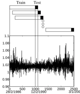
An illustration of the interaction of multiple objectives in a problem, where a set of models is desired for collective use (as opposed to comparison) can be shown by analogy to the CAPM from finance [20]. The CAPM describes the relation-ship between risk and return in an optimum portfolio of stocks, where risk is to be minimised and return maximised, and can therefore also be applied to populations of forecast models.
X X X X X X X X X X X X X X X X X X X X X X X X X X X X X X X X X X X X X X X X X X X X X X X X X X X X X X X X X X X X XX X X Risk Return S S F F Rf Rm a Sm
Fig. 3. The CAPM.
In Figure 3, the frontl+l represents the Pareto optimal
port-folios (called efficient portport-folios in CAPM), or forecast models in the analogy, with examples of other sub-optimal portfolios
(models) lying beneathl+l also marked. Linemnm is the
secu-rity market line, with pointo+p , where the security market line
intersects the y-axis, representing the level of ‘risk free’ return available in the market place to the individual (i.e. through borrowing/lending through the banking system). The secu-rity market line is tangential to the efficient portfolio front, the
point where it touches the front atq being the optimal
mar-ket portfolio. In the simple illustration shown in Figure 3, by
investing in the market portfolio at point q (by trading using
the forecast model at point q ) and lending or borrowing at
the risk free rateo+p , it is possible to operate on the security
market line, gaining a higher rate of return for any level of risk than that possible by investing in an efficient portfolio of stocks. More complex interactions can also be modeled within the CAPM framework. For example where there are two dif-ferent zero-risk rates in the market; that available to the user when borrowing, and that available from government bonds (risk-free investing). In this situation there are two tangential lines generated, with a ‘kinked’ Security Market Line itself a combination of the two and the front itself between the two tan-gents. In addition, given that different individuals/institutions
may experience differingo+p s (due to differing costs of
bor-rowing and lending available dependent on size and circum-stance), the tangential points themselves (and therefore specific models of interest) will vary across individuals.
V. DATA AND ERROR MEASURES
In this study two error measures to be optimised are ‘Risk’ (minimised) and ‘Return’ (maximised).
The dependent time series used for forecasting,2?r
, is a form of the one day return between the open price of the market and the next day realised high, as shown in eq. 9.
2 r 5ts u$v r w Dx4xy u$z r|{ -~} (9) whereu z r
is the open level of the market at day and
unv
r
is the
market high at day.
The multiplication of the open value by 0.993 is due to the trading strategy being dependent on the value falling during the day by at least 0.7% before trading into the market is (poten-tially) triggered (as described in Algorithm 1). The ‘Risk’ of a forecast model is simply measured as the Root Mean Squared
Error (RMSE) of the model prediction of2?r
- as it is a direct
measure of the (standard deviation) of the model prediction
from the actual. The ‘Return’ measure is calculated using a simple trading strategy based upon transaction costs calculated at 0.1% of price (as defined as a reasonable level in [21]), there-fore a minimum increase in price from buy to sell of 0.2% is needed before any profits can be realised. In addition the trad-ing strategy is designed such that a trade will only take place if estimated profits beyond transaction costs of a trade into and out of the market equal approximately 1.5% (the forecast of
2r
, 2r
being 1.017). The ‘Return’ error measure is formally
described in Algorithm 1.
Algorithm 1 Trading strategy (‘Return’ error).
, current time step (day).
2r
, the model forecast at day.
r 5 P <~ , whereu r
is the market close on day.
r
r
, Return value at time (as a percentage of capital at$
B
).
1. Set
5RB
, first trading day of train (or test) set instance.
2. If9 2rI - B4D w B=:K u rT u z r [ w Dx4xy
shift capital from risk free deposit into market at the point where the market price falls to 99.3% of open (incurring transaction costs), goto 3, otherwise goto 4.
3.
5
M
B
, Calculate profit / loss. (a) if 9I2 r
B4D
w
B=
, sell when market reaches the level
101.7% of that when entered,W
r r 5RBD~x4y , goto 2. Else: (b) if 9L2 r ^ BD w B4=
, sell at the end of day, ¡
r r 5 9Lr B¢= 9 w D£B w D¤Br = , goto 2. 4. 5 B
, Calculate nominal risk free interest accrued on
assets, r r 5 w D ww B¢¥
(compound equivalent to 4% p.a.), goto 1.
Halt process when end of train (or test) set is reached.
The measure shows that if the forecast of tomorrows high is 1.7% higher or more than 99.3% of today’s open price, and the price during today falls to (or below) a level of 99.3% of today’s open price, trading will occur (Algorithm 1). If this
sit-uation occurs, and the realised value of value of2MrI
- is greater
thanB
.017, then when the market level reaches the point of be-ing 1.7% above the price paid on entrance, the assets will be sold and profits realised (after costs incurred). If however the market level does not reach a level 1.7% above the price paid on entrance then the assets are disposed of at the end of the day,
with the potential for either profit or loss. Ifu¦
rT u z r¨§ w Dx4xy , or 24rI -^©B4D w B
then no trade will occur and the capital will lie in a bank deposit accruing the equivalent of 4% interest p.a. (w
D
w4w B¥«ª
a day compounded over 250 trading days).
Fifteen explanatory variables were used in the model, and are defined as follows:
¬ -® )) - r 5G2r|{ / >DDD>2r|{ -P- (10) ¬ -P- )) -T¯ r 5 24r|{ ->DDD> 2r|{ ¯ (11)
variables 1 to 10 contain the last 10 lagged realised values of2 r
(2 weeks of trading), of course2 r|{
- cannot be used as it
incor-porates information that will not be available at the start of day atA
B
. Variables 11 to 15 are recurrent variables. In addition to the 15 input units, the network design used incorporated a single hidden layer of 5 sigmoidal transfer units.
The data used in the model is the open, high, low and close of the Dow Jones Industrial Average (DJIA) over the 2500 trading day period from 28/2/1986 to 3/1/2000. In (the Ex-perimentation) Section VI a sliding window is used to contain the training and test sets which are generated by first creating the relevant explanatory vector and dependent value pairs (em-bedded matrix), and then passing a window with the first 1000 pairs as training data and the next 100 pairs as test data across the series, moving the window forward by 100 pairs 25 times. As illustrated in Figure 4 below, this means that the 25 test sets contain a total of 1500 trading days (approximately 10 years) from 12/2/1990 to 3/1/2000. 0 500 1000 1500 2000 2500 0.96 0.98 1 1.02 1.04 1.06 1.08 1.1 28/2/1986 12/2/1990 3/1/2000 Train Test
Fig. 4. Figure illustrating the test and training sets (top) in relation to the transformed data°± (bottom).
VI. EXPERIMENTS AND RESULTS
The experiments in this study are designed to demonstrate the feasibility of this new approach to forecasting, and the ben-efit of producing a population of models which lie on an esti-mate of the Pareto front of the generating process. As stated, this allows the practitioner to choose a model from a viable set that describes a their error trade-off preferences after training and therefore knowledge of the training error interactions (in-stead of the approach of summation, where only one model is returned and where the practitioner must have a priori knowl-edge of the error surface). However, if the error properties do not hold true on the test data, this approach is of no use in the financial domain.
To test this three preferences of three general practitioners are defined (risk averse, profit maximiser and middle-way) and the relevant models for each of these type of investor selected at each of the training windows and the performance of the rel-evant model evaluated on the following test set. The risk averse model practitioner is represented by the lowest ‘Risk’ (RMSE) model from the Pareto model set being selected at each pe-riod. The profit maximising practitioner is represented by the highest ‘Return’ model selected at each period and the mid-dle practitioner (neither totally risk averse nor totally expected profit maximising) being represented by the middle model in the ordered model set at each window period.
The Genetic Algorithm used in the SPEA was implemented using single-point crossover, the mutator variable was drawn from a zero-mean, symmetric, leptokurtic distribution (kurto-sis ²
B
w
) generated by the product of two uniform distribu-tions covering the range [0,1], and a Gaussian distribution with a variance of 0.1 and zero mean. The probability of mutation was 0.1 and the probability of crossover 0.8. The search pop-ulation contained 80 individuals, with an unconstrained elite secondary population used as a source of up to 20 individuals each generation for the binary tournament selection phase of the SPEA (the algorithms and data structures used to facilitate this can be found in [22], [23]). Each population of networks was trained for 2000 generations, with the search population in each instance seeded with the search population at the end of the previous training window (the very first training window’s search population being randomly generated).
The average ‘Risk’ and ‘Return’ for the three practitioners as well as the market return and the performance of the
random-walk forecast of2~r
for the 25 test sets are shown in Table I.
(Again, as2 r
is not known at day, the random walk model
takes the form
2 r 52 r|{ / ).
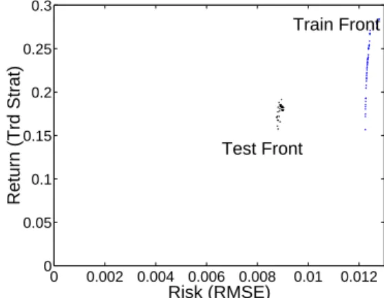
As can clearly be seen, the model attributes over the train-ing data are consistent over the test data also, although with a degree of noise. An example of this is illustrated in Fig-ure 5, with the training Pareto front and estimated test Pareto front plotted for the first training and test window. The mean ‘Risk’ of the central models’, although above that of the risk averse models on the test sets, is not significantly so. However the central models’ mean ‘Return’ is significantly higher, as are the profit maximisers models’ ‘Return’ significantly higher
TABLE I
MEAN RISK AND RETURN OVER THE25TEST SETS FOR THE EXTREME AND MID-WAY MODELS,RANDOM WALK MODEL AND
MARKET RETURN(STD DEVS IN PARENTHESIS).
Train Test
RMSE % Ret RMSE % Ret Risk 0.00903 0.1391 0.00923 0.0907 Averse (0.00181) (0.0306) (0.00316) (0.0742) Middle 0.00908 0.2299 0.00923 0.1714 (0.00182) (0.0569) (0.00308) (0.1317) Prof. 0.00927 0.2904 0.00978 0.2233 Max. (0.00184) (0.0797) (0.00302) (0.1780) Market - 0.0508 - 0.0619 - (0.0208) - (0.0717) Rand 0.01348 0.1293 0.01295 0.1175 Walk (0.00312) (0.0364) (0.00461) (0.0968) RiskFree 0 0.0016 0 0.0016
than both the central models’ ‘Return’ and minimal risk mod-els ‘Return’. (Calculated using the nonparametric Wilcoxon Signed Ranks Test [24] at the 2% level (1% in each tail)).
0 0.002 0.004 0.006 0.008 0.01 0.012 0 0.05 0.1 0.15 0.2 0.25 0.3 Risk (RMSE) Return (Trd Strat) Test Front Train Front
Fig. 5. Estimated Pareto error surface on training set and the noisy error surface realised on the test set (first window).
The tabulated results are further supported in a visual fash-ion by the Profit plots over the 10 year period for the vari-ous models, which are shown in Figure 6. It is of interest to note that all three NN model types outperform the market re-turn, however the risk averse models (RMSE minimiser) dis-play a lower return over the period than the simple random walk model on the transformed data, once more underlining the fact that models should be trained with respect to the er-ror preferences of the user (models trained strictly to minimise RMSE will not necessarily generate excess profits).
VII. COMMENTS AND FURTHER WORK
In this study a novel approach to the construction of finan-cial time series models has been formed by analogy with the CAPM from portfolio theory. Approximate Pareto frontiers have been generated for the DJIA index based on NN model
0 500 1000 1500 2000 2500 0 0.5 1 1.5 2 2.5x 10 4 Trading Days Capital 12/2/1990 3/1/2000 Market Ret. Lowest Risk NN Random Walk Mid Risk/Ret. NN Max Ret. NN
Fig. 6. Profit plots for the 10 year test period for the extreme and mid models on the training Pareto front, the random walk model and the market return (capital initialised at 100).
risk and return. As a result of this it has also been demon-strated that risk and return are non-commensurable in model parameter specification, and that this generalises to test data.
However there are still many further areas of research in this field. Both [16] and this study do not fully confront the prob-lem of generalisation / validation in the domain of Pareto pop-ulation training. The MOEA literature was formed in ‘clean’ process domains. In noisy domains such as financial fore-casting, where the generating process itself is being modelled, the divergence between the estimated Pareto surface from the training data, and the actual surface defined by the process it-self merits much further investigation. In addition there is no reason to assume that the population of NN models defining the front should be homogeneous in their topologies, indeed, just as it is accepted that no one NN topology is optimal for a num-ber of different tasks - so it may also be assumed that no one NN topology is sufficient for representing diverse and compet-ing error representations of a scompet-ingle noisy process. These, and other areas, are the focus of the author’s current research.
VIII. ACKNOWLEDGMENTS
Jonathan Fieldsend gratefully acknowledges support from Inven-sys Climate Controls Europe and an Exeter University Studentship. The software for this work used the GAlib genetic algorithm pack-age, written by M. Wall at the Massachusetts Institute of Technology (http://lancet.mit.edu/ga).
References
[1] M. Adya and F. Collopy. How Effective are Neural Networks at Fore-casting and Prediction? A Review and Evalution. International Journal
of Forecasting, 17:481–495, 1998.
[2] J. Moody. Forecasting the Economy with Neural Nets: A survey of Chal-lenges and Solutions. In G.B. Orr and K-R Mueller, editors, Neural
Net-works: Tricks of the Trade, pages 347–371. Berlin: Springer, 1998.
[3] A-P.N. Refenes, A.N. Burgess, and Y. Bentz. Neural Networks in Fi-nancial Engineering: A Study in Methodology. IEEE Transactions on
Neural Networks, 8(6):1222–1267, 1997.
[4] S. DeLurgio. Forecasting: Principles and Applications. McGraw-Hill, 1988.
[5] J.E. Fieldsend. Non-linear ARCH Volatility Estimation Using Neural Networks. Master’s thesis, University of Plymouth, 1999.
[6] D. Gujarati. Essentials of Econometrics. McGraw-Hill, 1992. [7] J.S. Armstrong and F. Collopy. Error measures for generalizing about
forecasting methods: Empirical comparisons. International Journal of
Forecasting, pages 69–80, 1992.
[8] Y. Wang and F.M. Wahl. Multiobjective neural network for image re-construction. IEE Proceedings - Vision, Image and Signal Processing, 144(4), 1997.
[9] C-G. Wen and C-S Lee. A neural network approach to multiobjective optimization for water quality management in a river basin. Water
Re-sources Research, 34(3):427–436, 1998.
[10] J. Yao and C.L. Tan. Time dependant Directional Profit Model for Fi-nancial Time Series Forecasting. In IJCNN 2000, Proceedings of the
IEEE-INNS-ENNS International Joint Conference on Neural Networks,
2000.
[11] E.W. Saad, D.V. Prokhorov, and D.C. Wunsch. Comparitive Study of Stock Trend Prediction Using Time Delay, Recurrent and Probabilistic Neural Networks. IEEE Transactions on Neural Networks, 9(6):1456– 1470, 1998.
[12] C.A.C Coello. A Comprehensive Survey of Evolutionary-Based Mul-tiobjective Optimization Techniques. Knowledge and Information
Sys-tems. An International Journal, 1(3):269–308, 1999.
[13] C.M. Fonseca and P.J. Fleming. An Overview of Evolutionary Al-gorithms in Multiobjective Optimization. Evolutionary Computation, 3(1):1–16, 1995.
[14] D. Van Veldhuizen and G. Lamont. Multiobjective Evolutionary Al-gorithms: Analyzing the State-of-the-Art. Evolutionary Computation, 8(2):125–147, 2000.
[15] J.D. Schaffer. Multiple objective optimization with vector evaluated ge-netic algorithms. In Proceedings of the First International Conference
on Genetic Algorithms, pages 99–100, 1985.
[16] M.A. Kupinski and M.A. Anastasio. Multiobjective Genetic Optimiza-tion of Diagnostic Classifiers with ImplicaOptimiza-tions for Generating Receiver Operating Characterisitic Curves. IEEE Transactions on Medical
Imag-ing, 18(8):675–685, 1999.
[17] J. Horn, N. Nafpliotis, and D.E. Goldberg. A Niched Pareto Genetic Algorithm for Multiobjective Optimization. In Proceedings of the First
IEEE Conference on Evolutionary Computation, IEEE World Congress on Computational Intelligence, volume 1, pages 82–87, Piscataway, New
Jersey, 1994. IEEE Service Center.
[18] E. Zitzler, K. Deb, and L. Thiele. Comparison of Multiobjective Evo-lutionary Algorithms: Empirical Results. EvoEvo-lutionary Computation, 8(2):173–195, 2000.
[19] V. Pareto. Manuel D’ ´Economie Politique. Marcel Giard, Paris, 2nd
edition, 1927.
[20] R.A. Brealey and S.C. Myers. Principles of Corporate Finance.
McGraw-Hill, 5th edition, 1996.
[21] C. Schittenkopf, P. Tino, and G. Dorffner. The profitability of trading volatility using real-valued and symbolic models. In
IEEE/IAFE/INFORMS 2000 Conference on Compuational Intelligence for Financial Engineering (CIFEr), pages 8–11, 2000.
[22] J.E. Fieldsend, R.M. Everson, and S. Singh. Extensions to the Strength Pareto Evolutionary Algorithm. IEEE Transactions on Evolutionary Computation, (submitted), 2001.
[23] R.M. Everson, J.E. Fieldsend, and S. Singh. Full Elite-Sets for Multi-objective Optimisation. In Proceedings of the fifth internatioanl
confer-ence on adaptive computing in design and manufacture (ACDM 2002).
Springer-Verlag (to appear), 2002.
[24] F. Wilcoxon and R.A. Wilcox. Some Rapid Approximate Statistical