A new resampling method for sampling designs without
replacement: the doubled half bootstrap
Erika Antal · Yves Tillé
Abstract A new and very fast method of bootstrap for sampling without replacement from a finite population is proposed. This method can be used to estimate the variance in sampling with unequal inclusion probabilities and does not require artificial popu-lations or utilization of bootstrap weights. The bootstrap samples are directly selected from the original sample. The bootstrap procedure contains two steps: in the first step, units are selected once with Poisson sampling using the same inclusion probabilities as the original design. In the second step, amongst the non-selected units, half of the units are randomly selected twice. This procedure enables us to efficiently estimate the variance. A set of simulations show the advantages of this new resampling method. Keywords Poisson sampling·Simple random sampling ·Unequal probability sampling·Variance estimation
1 Introduction
Resampling methods are frequently used to draw inference in survey statistics. The main difficulty, however, is that the variance of an estimator depends on the sampling design. Bootstrap methods must thus be adapted for each sampling design. Moreover, the variance of the Horvitz–Thompson estimator can have a very different form from
E. Antal
Swiss Centre of Expertise in the Social Science,
Quartier UNIL-Mouline, Bâtiment Géopolis, 1015 Lausanne, Switzerland e-mail: [email protected]
E. Antal·Y. Tillé (
B
)Faculty of Economics and Business, Institute of Statistics, University of Neuchâtel, Rue de la Pierre-à-Mazel 7, 2000 Neuchâtel, Switzerland
e-mail: [email protected]
Published in Computational Statistics 29, issue 5, 1345-1363, 2014 which should be used for any reference to this work
the variance estimator. The original bootstrap method, developed by Efron (1979) i s not directly applicable in sampling from a finite population because the units of the sample are not independent and identically distributed when the sample is selected
without replacement. Gross (1980), Booth et al. (1994) and Chao and Lo (1985)
proposedamethodbasedontheconstructionofpseudo-populationsfromthesample
(seealsothegeneralizationsofChauvet2007).Anotherimportantfamilyofmethods
istherescaledbootstrap(RaoandWu1988)whichconsistsofmodifyingthevalues
oftheinterestvariabletoreconstructanunbiasedvarianceestimatorforstatisticsthat
are linear functionsof the observations. The Rao andWu methodcan however be
alsopresentedasaweightingsystem(Raoetal.1992)thatisappliedonthevectorof the variable of interest. Other methods were also proposed by Mac Carthy and Snowden (1985), Kuk (1989), Rao et al. (1992), Shao and Tu (1995), Sitter (1992a), Sitter (1992b), Holmberg (1998).
The main idea of this paper is similar to the general weighted bootstrap (Mason and Newton 1992; Bertail and Combris 1997), which has also been used in the paper of Lahiri (2003). Beaumont and Patak (2012) propose a bootstrap method that directly reconstructs thevariance for linear cases.Antal and Tillé (2011a) propose anothermethodthatusesnon-integerweightsandthatisbasedonmixtureofdiscrete multi-variate distributions. In this paper, we propose a new methodology to select a bootstrap sample for sampling without replacement from a finite population. This method is an extension of the half-sample bootstrap proposed by Saigo et al. (2001) towhichweadd acorrection forfinitepopulationinorder tocorrectlyestimate the
variance in unequal probability sampling. This method enables one to quickly
implement and directly reconstruct the appropriate variance without need of
reweighting the statistical units. Indeed, each unit is duplicated an integer number of times.
The paper is organized as follows: in Sect. 2, the notation for a sampling design, the estimator of the total and its variance estimator are defined. Section 3 is devoted totheconditionsneededtoobtainunbiasedbootstrapestimatesofthevariances.In
Sect. 4, a new method is proposed for Poisson sampling. Next, the doubled half
samplingisdefinedinSect.5.Thistoolisusedtodefineanewbootstrapmethodfor
simplerandomsamplinginSect.6 andforunequalprobabilitysamplinginSect. 7.
Simulations are presentedinSect.8andtheinterestofthisnewmethodisdiscussed in Sect. 9.
2 Sampling design, total and variance
Let p(.)be a sampling design on a population U = {1, . . . ,N}of size N such that
p(s)≥0, for all s⊂U, and
s⊂U
p(s)=1.
Let S be the random sample such that Pr(S=s)=p(s).The sample size n of S can be random or not. Define also the inclusion probabilitiesπk =Pr(k∈ S)for k ∈U, and the joint inclusion probabilitiesπk =Pr(k and∈ S)for k, ∈U.Moreover, definek=πk−πkπfor k, ∈U,andkˇ =k/πk.When k=,we obtain
Several other variance estimators exist. They all have the same form as the SYG-estimator with different values for Dk. Matei and Tillé (2005) discussed the merits
of a family of estimators based on another value of Dkgiven by:
Dk= ⎧ ⎪ ⎪ ⎪ ⎪ ⎨ ⎪ ⎪ ⎪ ⎪ ⎩ ck− c 2 k j∈Scj if k= −ckc j∈Scj if k=.
Diverse values have been proposed for the ck. Matei and Tillé (2005) ran a set of
simulations that shows that the choice proposed by Hájek (1981):
ck = n
n−1(1−πk). (4)
produces a very efficient and slightly biased estimator. We refer to this estimator as the H-estimator of the variance.
3 Bootstrap
A bootstrap sample is a sample with replacement that is not necessarily a simple random sample and that is selected from S. Let S∗k be the number of times unit k is repeated in the bootstrap sample. The HT estimator of the total for a single bootstrap sample is given by Y∗= k∈S yk πkSk∗.
Let Pr∗(.)=Pr(.|S), E∗(.)=E(.|S), var∗(.)=var(.|S)and cov∗(., .)=cov(., .|S)
respectively denote the probability, the expectation, the variance and the covariance operators in the bootstrap sample conditional on the original sample. This gives us
E∗(Y∗)= k∈S yk πkE(Sk∗), and var∗(Y∗)= k∈S ∈S yky πkπcov ∗(S∗ k,S∗).
A necessary and sufficient condition for the expected value E∗(Y∗)to equal the HT estimator of the total is
E∗(Sk∗)=1,k∈ S. (5)
Moreover, in order to have an unbiased bootstrap estimate of the variance of the HT total estimator, we can define a bootstrap method such that the variance of the
bootstrap estimators of the total is equal to the HT variance estimator given in (1). In order to satisfy this equality, the necessary and sufficient condition is composed of two parts. The first condition is that
var∗(Sk∗)= ˇkk=1−πk,k∈ S. (6) The second condition is that
cov∗(Sk∗,S∗)= ˇk,k=∈S. (7)
The condition on the covariancesis however difficult tomeet when the sample is
selectedwithfixedsamplesizeandunequalinclusionprobabilities.Inthisparticular case,itisdifficulttoexactlysatisfymorethanconditions(5)and(6).Condition(7) canhoweverbeapproximatelysatisfied.
When the sample size is fixed, another way of constructing an unbiased estimator of the variance is to equalize the variance of the bootstrap estimator of the total with the SYG-estimators of the variance. The conditions become
E∗(Sk∗)=1,k∈S, (8)
var∗(Sk∗)=Dkk,k∈ S, (9)
and
cov∗(Sk∗,S∗)=Dk,k=∈S. (10) But again, conditions (10) on the covariances are difficult to meet when the sample is selected with unequal inclusion probabilities, but it could be approximately satisfied. For unequal probability sampling with fixed sample size, there exist two bootstrap strategiesthatmaybeusedtoapproximateeithertheHTortheSYG-estimator.
The bootstrap estimator of the variancevboot(Y∗)is computed by generating a set of bootstrap samples and by computing the variance of the outcomes ofY∗.Moreover, if a bootstrap method provides an approximately unbiased estimator for the variance of totals, it will also provide approximately unbiased variance estimators for smooth functions of totals.
Thereexistsalotofdistributionsthatsatisfyconditions(5)and(6) o r ( 8)and (9).However,iftheoriginalsampleisselectedwithunequalinclusionprobabilities and
if we impose that Sk∗is integer and that the sum of the Sk∗is not random, the problem is really complex. This is a problem of sampling with replacement and with unequal probabilities where the expectation and the variance are fixed. For this reason let us begin with a simple case: Poisson sampling design.
4 Bootstrap for Poisson design
Suppose the original sample is obtained by a so-called Poisson design, where the obser-vation k is included with probabilityπkand the decision is made for each observation independently. The name reflects the fact that if allπkare small, then the sample size
n has approximately a Poisson distribution with meankN=1πk. In a Poisson design with inclusion probabilitiesπk,
p(s)= N k=1 π1(k∈s) k (1−πk)1( k∈/s), for all s⊂U,
where 1(A)is equal to 1 if A is true and 0 otherwise. The inclusion probability is Pr(k ∈ S) = πk. Moreover,πk = πkπ when k = ∈ U and πkk = πk. Thus
k =0,when k = ∈U andkk =πk(1−πk).We thus have,kˇ =0,when
k = ∈ U andkkˇ =1−πk.With Poisson sampling design the sample size n is random thus the estimator of variance is calculated byvarH T(Yπ).
Patak and Beaumont (2009) propose a bootstrap method for Poisson design that use several different distribution as normal or lognormal random variables with expectation equal to 1 and variances equal to 1−πk. Unfortunately, this method requires the use of non-integer weights. Instead we recommend the use of a discrete random variable for Sk∗.
Antal and Tillé (2011a) propose a simple bootstrap method that uses n independent
Bernoulli random variables Xkwith parameterπkand n independent Poisson random
variables Zkwith parameterλ=1.For this method, the bootstrap sample is given by Sk∗=Xk+(1−Xk)Zk,k∈S.
Thus, the probability mass function of Sk∗is given by:
Pr∗(Sk∗=r)=πk1[r=1] +(1−πk)
e·r! ,r =0,1,2, . . .
wheree≈2.71istheEulerconstant.ThebootstrapvariableSk∗ satisfiesconditions (5),(6),and(7).
We propose another method based on n independent Bernoulli random variables
Xk,k ∈S with parameterπkand n independent Bernoulli random variables Yk with
parameter 1/2.Define the bootstrap sample by
Sk∗=Xk+2(1−Xk)Yk,k∈ S.
The probability distribution of Sk∗is thus
Sk∗= ⎧ ⎨ ⎩ 0 with a probability(1−πk)/2 1 with a probabilityπk 2 with a probability(1−πk)/2.
Again,thebootstrapvariableSk∗ meetsconditions(5),(6),and(7).Here,the bootstrap sample does not contain the same unit more than twice.
5 One-one design and doubled half sampling
When the original sample has a fixed sample size, Antal and Tillé (2011a) propose one-onedesigns,atoolinordertoestimatethevarianceofanestimatorviabootstrap method.Membersofthisfamilyarediscreteprobabilitydistributionswith
E∗(Sk∗)=1,
var∗(Sk∗)=1.
The name comes from these conditions on their expectation and variance. Each boot-strap sample has the same fixed sample size
k∈S
S∗k =n.
The covariance between Sk∗and S∗is given by
cov∗(Sk∗,S∗)= −
1
n−1,k=∈S.
AntalandTillé(2011a) showedthatsuch asamplingdesigncanbeobtained by
using a mixture between two samples selected by simple random sampling with
replacementandbysimplerandomsamplingwithover-replacement(AntalandTillé
2011b).One-onedesignscannextbemixedwithothersamplingdesignsinorderto
reproduce an unbiased estimator of variance for most of the sampling methods with fixed sample size.
We propose another method for selecting a one-one design that we call “doubled half sampling”. In the next section we use this in a new bootstrap procedure. If the size n of the initial sample is even, then a sample from S of size n/2 is selected with simple random sampling without replacement. Next, each selected unit is taken twice. In this case, we obtain
E∗(Sk∗)=2×1 2 =1, var∗(Sk∗)=4×1 2 1−1 2 =1, and cov∗(Sk∗,S∗)=4×1 2 1−1 2 −1 n−1 = −1 n−1.
If n is odd, then we can have the same property by means of the following slightly modified procedure:
• With a probability 1/4, select a unit with equal probabilities from the set of units selected twice. This unit is selected three times.
• Otherwise, with a probability 3/4, select a unit with equal probabilities among the units that are not selected twice. This unit is selected only once.
This procedure gives the following distribution for S∗k:
Pr∗(Sk∗= j)= ⎧ ⎪ ⎪ ⎪ ⎪ ⎪ ⎪ ⎪ ⎨ ⎪ ⎪ ⎪ ⎪ ⎪ ⎪ ⎪ ⎩ n+1 2n × 1−34×n+21 =2n−1 4n if j =0 n+1 2n × 3 4× 2 n+1 = 3 4n if j =1 n−1 2n × 1−14×n−21 =2n−3 4n if j =2 n−1 2n × 1 4× 2 n−1 = 1 4n if j =3.
After some algebra, it can be shown that this design is one-one. A one-one design can thus be selected for any sample size except when n=1.
6 Bootstrap for simple random sampling without replacement
In this section we propose a bootstrap method for use when original samples are selected by simple random sampling without replacement, where
p(s)=
n!(N−n)!
N! for all the samples s of size n
0 otherwise.
The inclusion probability isπk=n/N.Moreover,
πk= n(n−1)
N(N−1) when k=∈U andπkk=n/N . Thus,
k= − n(N−n) N2(N−1), when k=∈U and kk =n(N−n) N2 . We thus have, ˇ k = −NN(n−−n1),
when k =∈U andkkˇ =1−n/N.Note also that in this case, the HT-estimator and the SYG-estimator of the variance are equal, i.e.kkˇ =Dkk =1−n/N for all
k∈U.
We propose using bootstrap samples using the following two-stage procedure. Let
Sk∗denotes the number of times unit k is selected in the bootstrap sample.
• Select units from S by using independent Bernoulli random variables Xk,k∈ S,
with probabilitiesπk =n/N.Let m=k∈SXk.Thus E(m)=n2/N.For now
we set S∗k =Xk, including each selected unit in the bootstrap sample once, though this may be adjusted later.
• – If the number of non-selected units is greater than or equal to 2 (n−m≥2), then select a doubled half sampling design amongst the units k ∈S such that Xk =0.
– If there is exactly one (say unit) non-selected unit (n−m =1), select that unit with distribution
S∗= ⎧ ⎨ ⎩ 0 with probability 1/4 1 with probability 1/2 2 with probability 1/4.
Next, randomly select one of the units such that Xk = 1 (say z) with equal
probability and select it S∗z =2−S∗times.
– If the number of units such that Xk =0 is null (n−m=0), then the bootstrap
sample Sk∗is the same as the original sample. Note that Pr∗(Sk∗= j|m=r and n−r is even)= ⎧ ⎨ ⎩ (1−r/n)/2 if j =0 r/n if j =1 (1−r/n)/2 if j =2, Pr∗(Sk∗= j|m=r,n−r is odd, and r <n−1)= ⎧ ⎪ ⎪ ⎪ ⎪ ⎪ ⎨ ⎪ ⎪ ⎪ ⎪ ⎪ ⎩ 1−rn2n4n−1 if j =0 r n + 1−rn4n3 if j =1 1−rn2n4n−3 if j =2 1−rn4n1 if j =3, and Pr∗(S∗k = j|m=n−1)= ⎧ ⎨ ⎩ 1/(2n) if j =0 1−1/n if j =1 1/(2n) if j =2.
It can be checked that E(Sk∗|m)=1 and var(Sk∗|m)=1−m/n, for all three cases. We obtain E(Sk∗)=E[E(Sk∗|m)] =1 and
var(S∗k)=E var(Sk∗|m)
var∗(Sk∗)= ˇk=1−πk,k∈ S,
or, by posingφk =1−Dkk,
var∗(Sk∗)=Dkk=1−φk,k∈S.
With unequal inclusion probabilities, it is difficult to construct a bootstrap method that meets the properties of the covariances given by
cov∗(Sk∗,S∗)= ˇk, or cov∗(Sk∗,S∗)=Dk,k=∈S. (12) Nevertheless, since the bootstrap sample has a fixed sample size, the relation
k∈S
cov∗(Sk∗,S∗)=0 (13)
is the same as for Dk. Indeed, k∈S
Dk=0, (14)
whichensuresthat(12)willbeapproximatelysatisfiedwhenthesamplingdesignhas large entropy. Let Sk∗denotes the number of times unit k is selected in the bootstrap sample.
• Select units from S by using a Poisson random variable Xk,k∈ S,with the same inclusion probabilities as the original designπk.The selected units are taken once in the bootstrap sample Sk∗. For now we set Sk∗=Xk, including each selected unit in the bootstrap sample once, though this may be adjusted later. Let m=k∈SXk.
Thus E(m)=k∈Sπk.
• – If the number of non-selected units is greater than or equal to 2 (n−m≥2), then select a doubled half sampling design amongst the units such that Xk =0.
– If there is exactly one (say unit) non-selected unit (n−m =1), the Sk∗are completely redefined.
• With a probability 1/2, select the same bootstrap sample as the original sample (Sk∗=1,k∈ S).
• Otherwise, with a probability 1/2, compute
πk|n−1=E(Xk|m=n−1)=1− 1−πk πk ∈S 1−π π
(see the Appendix for the proof). With a sampling method with unequal inclusion probabilities with fixed sample size, select n−2 units from S with probability
and take them once in the bootstrap sample. Select a sample with a doubled half sampling from the two units that are not selected. Note thatψk = 2πk|n−1−1 except when one of theπk|n−1is less than 1/2.
NotethattheprocedureproposedinSect.6forsimplerandomsamplingisa particularcaseoftheprocedureforunequalprobabilitysamplingwhen πk=n/N. Result 1 With this procedure E(Sk∗|m)=1,
var(Sk∗|m=r)=1−πk|r,r=0,2,3, . . . ,n, var(S∗k|m=1)= 1−ψk 2 =1−πk|n−1+πk|n−1− 1+ψk 2 , whereπk|r =E(Xk|m=r).
The proof is given in the Appendix.
We thus have E(Sk∗)=E[E(Sk∗|m)] =1 and var(Sk∗)=Evar(Sk∗|m)+varE(Sk∗|m)
=E(1−πk|r)+ πk|n−1− 1+ψk 2 Pr∗(m=n−1) =1−πk+ πk|n−1− 1+ψk 2 Pr∗(m=n−1). The variance of the diagonal is very slightly biased. Indeed
var∗(Sk∗)= ˇkk+ πk|n−1− 1+ψk 2 Pr∗(m=n−1),k∈ S.
The bias is small and often nonexistent. Indeed,(m=n−1)is a rare event. Moreover,
πk|n−1−(1+ψk)/2 is null except if one of theπk|n−1is smaller than 1/2,which is also rare except in case where the sample size is very small. Moreover, we always have
k∈S πk|n−1− 1+ψk 2 =0.
Below, the simulations will show that even for very small sample sizes, the bias is negligible.
The same results can be derived by takingφkin place ofπk. The Dkkcan sometimes
be larger than 1. In this case, we advocate to takeφk = 0.We can thus define two bootstrap methods depending on whether the inclusion probabilities are πk or φk. The first case will be referred to asπ-bootstrap and the second asφ-bootstrap. The bootstrap sample size always remains fixed, i.e.
k∈S
Sk∗=n,
k∈S
E∗(Sk∗)=n and k∈S
cov∗(Sk∗,S∗)=0.
Unfortunately,wecannotshowtheoreticallythat(7) o r ( 10)aresatisfied,which areconditionsforthevalidityofbootstrapvarianceestimation.However,theeffect ofignoring(7) o r ( 10)isnotimportantinourempiricalstudy.Thisiscertainlydue tothefactthatthemarginalconstraintsgivenin(13)and(14)aresatisfied.
8 Simulation studies
8.1 Comparison with existing variance estimators for the total
In the first part of the simulation study, we examined the performance of the
estimator using the proposed method and then comparedthis estimator withother
varianceesti-mators.WeransimulationsontheMU284 populationfromSärndalet
al.(1992) f r o m whereweselectedsamplesofsizen=2,n=10andn=40with
inclusionprobabil-itiesproportionaltovariableP75(populationin1975).Weuseda
maximum entropy design (also called conditional Poisson sampling) because this
method maximizes the entropy of the sampling design subject to given inclusion
probabilitiesandfixedsample sizeandcanbeimplemented veryquickly(see Tillé
2006).ThevariableofinterestwasRMT85(revenuesfrom1985municipaltaxation).
WecomparedtheHT-estimator,theSYG-estimator,theH-estimator,the π-bootstrap
and the φ-bootstrap of the variance for the total of RMT85. We ran 10,000
simulationsand,ineachofthem,weused 10,000bootstrapreplications.Duetothe
simplicity of the method, the simulations were achieved in a few hours. Table 1
showstherelativebiasgivenby
RB= Esi m[vboot(Y
∗)] −var(Y) var(Y)
and the coefficients of variation given by
CV=
varsi m[vboot(Y∗)]
var(Y)
of the HT-estimator, SYG-estimator and the Bootstrap estimator, where Esi m(.)and
varsi m(.)respectively denote the expectation and the variance under the sample
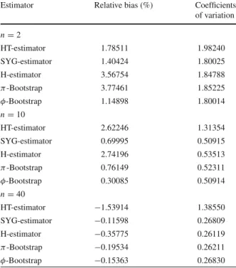
selec-tion mechanism estimated by the simulaselec-tions. Although only the HT-estimator and the SYG-estimator are strictly unbiased, the relative bias of theπ-bootstrap method given by the simulations is still smaller. All the bias computed by simulation are nevertheless very small and are not significantly different from zero. The simulations also show that the HT-estimator is very unstable and that the bootstrap method performs as well as the SYG-estimator and the H-estimator. These simulations show that the bootstrap leads to an estimator of the variance that is at least as efficient as the SYG-estimator even for a very small sample size (n=2).
Table 1 Relative bias and coefficients of variation of the HT-estimator, the
SYG-estimator, H-estimator, the
π-bootstrap and theφ-bootstrap
Estimator Relative bias (%) Coefficients
of variation n=2 HT-estimator 1.78511 1.98240 SYG-estimator 1.40424 1.80025 H-estimator 3.56754 1.84788 π-Bootstrap 3.77461 1.85225 φ-Bootstrap 1.14898 1.80014 n=10 HT-estimator 2.62246 1.31354 SYG-estimator 0.69995 0.50915 H-estimator 2.74196 0.53513 π-Bootstrap 0.76149 0.52311 φ-Bootstrap 0.30085 0.50914 n=40 HT-estimator −1.53914 1.38550 SYG-estimator −0.11598 0.26809 H-estimator −0.35775 0.26119 π-Bootstrap −0.19534 0.26211 φ-Bootstrap −0.15363 0.26830
8.2 Performance in the case of variance estimation of other functions of interest In the second part of the simulation study, we ran simulations in order to examine performance in relation to the variance of nonlinear functions of interest. Besides the total, the ratio of two totals, the median and the Gini index were also used as a function of interest. In the case of nonlinear statistics, the variances under the simulations, say the Monte Carlo variances were considered as the true variances of the estimators. A population of 150 units was generated from the model yk=(β0+β1xk1.2+σ εk)2+c, with xk = |ik|and ik ∼N(0,7),εk ∼N(0,1)andσ =15. The regression parameters
wereβ0 =12.5,β1=3 and c =4000. The model and its parameters were chosen intentionally to have a distribution for y similar to a lognormal, as it is often used for income distributions, with a correlated and positive explanatory variable x in the regression model. From this population, 1000 samples were drawn using, as in the previous section, a maximum entropy sampling design with unequal inclusion probabilities. Concerning the inclusion probabilities, they were calculated proportional to the values of a variable z, which was generated from equation z = y0.2p where p∼lnN(0,0.25). In this manner, the correlation between y and z is about 0.5. We knowingly used a large sample rate n/N =1/3 and a skewed population in order to better illustrate the performance of the tested bootstrap methods. From each of these samples, we calculated four statistics: the total, the median, the Gini index of variable
From each of the 1,000 initial samples, 1,000 bootstrapsamples were selected
using three different bootstrap methods. Besides the new bootstrap method, two
other resampling methods were tested. The first one is the generalization of the
bootstrapmethodwithoutreplacementproposedbyBoothetal.(1994)for unequal
inclusionprobabilities(Chauvet2007).ThisbootstrapmethodofBoothetal.(1994) is itselfa variant of the initial bootstrapwithreplacement methodthat consists of creatingan artificialpopulationfromthe initialsampleandthendrawingbootstrap
samples fromitwiththe samedesignas theinitialone(Gross1980; ChaoandLo
1985).Afterdrawingthebootstrapsamples,theestimatorsandtheirvarianceswere computedforeachoftheinitialsamplesandthenthemeansofthesevarianceswere thencomparedwiththeapproximationsofthetruevariances.Notethatthemedianis notasmoothfunctionofthetotal.Estimatingitsvariancecanthereforebedifficult,
but the simulations show that in this case bootstrap methods perform well. The
secondoneisthemethodproposedinAntalandTillé(2011a).
In order to measure the performance of the new method and compare it with the other ones, the following five indicators were used:
• Lower error rate (L) in %
L= 100 si m si m i=1 I θ−1.96× var(θ∗) > θ ,
where I[a] =1 if a is true and I[a] =0 elsewhere, • Upper error rate (U) in %
U = 100 si m si m i=1 I θ+1.96× var(θ∗) < θ .
• Total error rate (ER) in %
E R=100− 100 si m si m i=1 I θ−1.96× var(θ∗)≤θ≤θ+1.96× var(θ∗) . • Relative Bias R B=100×var(θ ∗)−varsi m(θ) varsi m(θ) =100× B varsi m(θ) ,
where B is the Bias of the var(θ∗). • Relative Root Mean Squared Error
R R M S E =100×
B2+var[var(θ∗)] varsi m(θ)
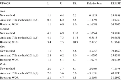
Table 2 Performance of the resampling methods in maximum entropy sampling design
UPWOR L U ER Relative bias RRMSE
1.1 6.4 7.5 0.1121 35.4938 0.6 6.2 6.8 −1.3094 33.9250 1.1 6.9 8.0 −1.6084 34.7805 4.1 6.9 11.0 −1.0564 58.8889 4.1 7.3 11.4 −6.5615 50.6651 3.4 7.5 10.9 2.8753 61.9642 1.5 5.1 6.6 3.5753 39.4669 2.8 6.2 9.0 −1.0795 35.4389 1.6 5.1 6.7 −1.0276 30.9325 2.0 3.7 5.7 2.0403 41.1975 2.0 3.6 5.6 −3.1038 40.1890 Total Newmethod
AntalandTillémethod(2011a,b) BootstrapWOR
Median Newmethod
AntalandTillémethod(2011a,b) BootstrapWOR
Gini Newmethod
AntalandTillémethod(2011a,b) BootstrapWOR
Ratio Newmethod
AntalandTillémethod(2011a,b)
BootstrapWOR 2.1 4.7 6.8 −2.8664 38.2802
The RB gives a measure of the bias of the estimator of variance. The RRMSE measures its accuracy and in the case of unbiasedness of the variance estimator it is equal to the variation coefficients. The Error Rates allow us to evaluate the capacity of the methods to provide a valid inference. The lower and the upper error rates give us an idea of how skewed the distribution of the estimatorθis.
Table 2 presents the results of the application of the resampling methodsfor a
maximumentropydesignwithinclusionprobabilitiesproportional tovariable z. I n
theproposedbootstrapmethod,theHájekapproximationgivenin(4)isused,which
givesus φk=πk.Eachmethodprovideconfidenceintervalsaround93–94%forthe
total, theratioandtheGiniindex,and89–90% forthe median.Thecolumnofthe
relativebiasesdirectlyshowsthat, ineachcaseof thefourfunctionsof interest,the methodsperformwellandgiverelativebiasesof1–3%.
Note that a high underestimation of the variance of a function of interest could result in a low coverage rate, and therefore high error rates for the function of interest, which is probably the case here. Regarding the relative root mean square errors, the same trend can be observed. The three treated method perform identically, giving a value of RRMSE around 30–40 % for the total, the Gini index and the ratio and 60 % for the median. In general, there is no major difference in performance between the proposed methods, the estimators are unbiased, or have a slight bias for each function. The RRMSE have the same order and the error rates show a slightly positively skewed distribution, with coverage rates between 90 and 95 %.
The new method thus provides essentially the same results as the other mentioned methods, but its application is simpler: it does not require a correction factor or artificial
population. Besides having at least the same performance as the method of artificial populations, its main advantage is that it is easy to implement and fast. Thus, the samples can be directly used to compute the variance of the functions of interest.
9 Discussion and interest of the method
Thenewmethodprovides similarresultsas theAntalandTillé(2011a)methodsby
usingamixtureofseveralsamplingdesigns.Theybothsatisfyconditions(5)and(6) o r (8)and(9).Theproposedmethodissimplerbecauseitiseasiertoimplement.Mainly thedoubledhalfbootstrapconsistsofselectingtwicehalfthesample,whichis partic-ularlysimple.Moreoverthedoublehalfbootstraplimitsthenumberofreplicationof theunitsinthebootstrapsample(maximun3andmainly2).
If the Sk∗are not integer, they define a bootstrap weighting system. The interest of a bootstrap method that uses a discrete random variable Sk∗is that a bootstrap sample can be defined. Each unit is simply replicated Sk∗times. The units of the bootstrap samples have the same Horvitz–Thompson weights as in the original sample.
These bootstrap methods compare favorably with the best of the classical variance estimates for linear statistics, and also apply to nonlinear statistics. Its simplicity, its speed and its efficiency speak in its favour. The bootstrap sample does not need to be reweighted. There is no need for artificial populations and extreme samples are also avoided because the units can be repeated twice or rarely three times. The bootstrap samples can directly be used to provide estimates.
Acknowledgments We are grateful to a referee for his/her very pertinent comments that helped us to improve the quality of this manuscript. This research was performed when Erika Antal was research assistant at the University of Neuchâtel.
Appendix
Lemma 1 If a sample S is selected by a Poisson sampling design with inclusion
probabilitiesπk in a population U of size N , if ns denotes the random sample site, then πk|N−1=Pr(k∈ S|nS=N−1)=1− 1−πk πk ∈U 1−π π . Proof We have Pr(k∈/S and nS=N−1)=(1−πk) =k π=1−πkπk ∈U π. Thus Pr(nS=N−1)= k∈U Pr(k∈/ and nS=N−1)= k∈U 1−πk πk ∈U π,
which gives the complementary of the conditional probability of Lemma 1. Pr(k∈/S|nS =N−1)=Pr(k∈/S and nS=N−1) Pr(nS=N−1) = 1−πk πk ∈U 1−π π .
Lemma1.canalsobederivedfromExpression(5.12)ofResult22inTillé(2006). Proof of Result 1
Proof Let πk|r=E(Xk|m =r).Theseconditionalprobabilitiesarenoteasyto
com-pute.ArecursiverelationforcomputationisgivenforinstanceinTillé(2006,p.81). Fortunately,wedonothavetocomputethisconditionalexpectationinordertoproof
the result except for case r = n −1. However we will use it in the following
reasoning.Wehave Pr∗(Sk∗= j|m=r and n−r is even)= ⎧ ⎨ ⎩ (1−πk|r)/2 if j=0 πk|r if j=1 (1−πk|r)/2 if j=2, Pr∗(S∗k=j|m=r,n−r is odd, and r <n−1)= ⎧ ⎪ ⎪ ⎨ ⎪ ⎪ ⎩ 1−πk|r 2n−1 4n if j=0 πk|r+ 1−πk|r 3 4n if j =1 1−πk|r 2n−3 4n if j =2 1−πk|r 1 4n if j=3, and Pr∗(Sk∗= j|m=n−1)= ⎧ ⎨ ⎩ (1−ψk)/4 if j =0 (1+ψk)/2 if j =1 (1−ψk)/4 if j =2. References
Antal E, Tillé Y (2011a) A direct bootstrap method for complex sampling designs from a finite population. J Am Stat Assoc 106:534–543
Antal E, Tillé Y (2011b) Simple random sampling with over-replacement. J Stat Plan Inference 141:597–601 Beaumont J-F, Patak Z (2012) On the generalized bootstrap for sample surveys with special attention to
poisson sampling. Int Stat Rev 80(1):127–148
Bertail P, Combris P (1997) Bootstrap généralisé d’un sondage. Annales d’Economie et de Statistique 46:49–83
Booth JG, Butler RW, Hall P (1994) Bootstrap methods for finite populations. J Am Stat Assoc 89:1282– 1289
Brewer KRW, Donadio ME (2003) The high entropy variance of the Horvitz–Thompson estimator. Surv Methodol 29:189–196
Brewer KRW, Hanif M (1983) Sampling with unequal probabilities. Springer, New York Chao MT, Lo SH (1985) A bootstrap method for finite population. SankhyA 47:399–405¯
Chauvet G (2007) Méthodes de bootstrap en population finie. PhD thesis, Université Rennes 2 Efron B (1979) Bootstrap methods: another look at the jackknife. Ann Stat 7:1–26
Gross ST (1980) Median estimation in sample surveys. In: ASA proceedings of the section on survey research methods. American Statistical Association, pp 181–184
Henderson T (2006) Estimating the variance of the Horvitz–Thompson estimator. Master’s thesis, School of Finance and Applied Statistics, The Australian National University
Holmberg A (1998) A bootstrap approach to probability proportional-to-size sampling. In: ASA proceedings of the section on survey research methods. American Statistical Association, pp 378–383
Horvitz DG, Thompson DJ (1952) A generalization of sampling without replacement from a finite universe. J Am Stat Assoc 47:663–685
Kuk AYC (1989) Double bootstrap estimation of variance under systematic sampling with probability proportional to size. J Stat Comput Simul 31:73–82
Lahiri P (2003) On the impact of bootstrap in survey sampling and small-area estimation. Stat Sci 18:199– 210
Mac Carthy PJ, Snowden CB (1985) The bootstrap and finite population sampling. Public Health Service Publication, Technical report
Mason D, Newton MA (1992) A rank statistic approach to the consistency of a general bootstrap. Ann Stat 20:1611–1624
Matei A, Tillé Y (2005) Evaluation of variance approximations and estimators in maximum entropy sam-pling with unequal probability and fixed sample size. J Off Stat 21(4):543–570
Patak Z, Beaumont J-F (2009) Generalized bootstrap for prices surveys. In paper presented at the 57th Session of the International Statistical Institute, Durban, South-Africa
Preston J, Henderson T (2007) Replicate variance estimation and high entropy variance approximations. In Papers presented at the ICES-III, June 18–21, 2007, Montreal, QC, Canada
Rao JNK, Wu CFJ (1988) Resampling inference for complex survey data. J Am Stat Assoc 83:231–241 Rao JNK, Wu CFJ, Yue K (1992) Some recent work on resampling methods for complex surveys. Surv
Methodol 18:209–217
Saigo H, Shao J, Sitter RR (2001) A repeated half-sample bootstrap and balanced repeated replications for randomly imputed data. Surv Methodol 27(2):189–196
Särndal C-E, Swensson B, Wretman JH (1992) Model assisted survey sampling. Springer, New York Sen AR (1953) On the estimate of the variance in sampling with varying probabilities. J Indian Soc Agric
Stat 5:119–127
Shao J, Tu D (1995) The jacknife and bootstrap. Sprinter, New York
Sitter RR (1992a) Comparing three bootstrap methods for survey data. Can J Stat 20:135–154 Sitter RR (1992b) A resampling procedure for complex survey data. J Am Stat Assoc 87:755–765 Tillé Y (2006) Sampling algorithms. Springer, New York
Yates F, Grundy PM (1953) Selection without replacement from within strata with probability proportional to size. J R Stat Soc B15:235–261