Support Vector Machine (SVM) aggregation modelling for spatio-temporal air pollution analysis

(1)

Support Vector Machine (SVM) Aggregation

Modelling for Spatio-temporal Air Pollution

Analysis

by

Shahid Ali

under the supervision of

Dr. Guillermo Ramirez-Prado and Dr. Simon

Dacey

Submitted to the Department of Computer Science

in partial fulﬁllment of the requirements for the degree of

Doctor of Computing

at the

UNITEC INSTITUTE OF TECHNOLOGY

Feb 2019

c

⃝

Shahid Ali, MMXIX. All rights reserved.

The author hereby grants to Unitec permission to reproduce

and to distribute publicly paper and electronic copies of this

thesis document in whole or in part in any medium now

known or hereafter created.

(2)

Abstract

This research addresses the spatio-temporal air pollution analysis problem. Existing air pollution studies often simplify the problem and fail to consider the fact that air

pollution is a spatial and temporal problem. More speciﬁcally, previous approaches are optimal for temporarily rich data; however, environmental data is more likely to

be collected over a large geographical area and at diﬀerent periods of time. This re-search proposes an approach based on a decentralised computational technique named

Scalable SVM Ensemble Learning Method (SSELM) for classifying air pollution data in Auckland in 2010 on an hourly basis. Special consideration is given to the

dis-tributed ensemble in order to resolve the spatio-temporal data collection problem. The proposed approach has been compared with SVM ensemble learning for air

pol-lution analysis in the Auckland region. Experiments demonstrated that the proposed SSELM approach outperforms SVM ensemble learning in eﬃciency and accuracy.

(3)

List of Abbreviations

ANN Applied Artiﬁcial Neural Network

AOVSR Accurate Online Support Vector Regression Model

API Air Pollution Index AQI Air Quality Index

ARC Auckland Regional Council BKS Behavior Knowledge Space

BLB Bag of Little Bootstraps

BPCA Bayesian Principal Component Analysis

CCI Correctly Classiﬁed Instances

CH4 Methane

CO Carbon Monoxide

CO2 Carbon Dioxide

DECORATE Diverse Ensemble Creation by Oppositional Relabeling Ar-tiﬁcial Training Examples

DS Dempster Shafer

DS Decision Stump

EEG Electroencephalography EL Ensemble Learning

EM Expectation Maximisation EPA Environment Protection Agency

EPIs Environmental Performance Indicators FFNN Feed Forward Neural Networks

FISs Fuzzy Interference Systems FN False Negative

FP False Positive

GMDH Group Method of Data Handling

GP Genetic Programming GSE Gaussian Estimation Error

(4)

ICI Incorrectly Classiﬁed Instances

IT2FNN Interval Type-2 Fuzzy Neural Network KS Kappa Statistics

LI Linear Interpolation LS-SVM Least Square SVM

LTP Linear Trend at Point

MAE Mean Absolute Error MAR Missing at Random

MDNP Median of Nearby Points MLP Multilayer Perceptron

MMSD Mean Method by Step Depression

MN Modular Network

MNP Mean of Nearby Points

MRESVM MapReduce based Distributed SVM Ensemble

MRI Magnetic Resonance Imaging

NIWA National Institute of Water and Atmospheric Research

NO2 Nitrogen Oxide

NNS Neural Networks

NT NB Tree

OSSELM Online Scalable SVM Ensemble Learning Method

O3 Ozone

OWA Order Weight Average

PAC Probably Approximately Correct PM10 Particulate matter

PCA Percentage Classiﬁcation Accuracy PCA Principal Components Analysis

PSO Particle Swarm Optimisation PSVM Proximal SVM

PWM Perceptron Weighted Majority RandT Random Tree

(5)

RBF Radial Basis Function

RCQ Recursive Quartiles RMSE Root Mean Square Error

RSM Response Surface Methodology

RT REP Tree

SalncSVR Spatial data aided incremental Support Vector Regression

SDT Single Decision Tree

SM Series Mean

SMM Series Mean Method

SMO Sequential Minimal Optimisation

SO2 Sulphur Dioxide

SVMs Support Vector Machines

TN True Negative

TP True Positive

(6)

List of Publications

Ali, S., Dacey, S., Online Scalable SVM Ensemble Learning Method (OS-SELM) for Spatio-temporal Air Pollution Analysis. International Journal of

Data Mining and Knowledge Management Process (IJDKP-2017).

Ali, S., Dacey, S., Technical Review: Performance of Existing Imputation

meth-ods for Missing Data in Ensemble Creation. International Journal of Data Mining and Knowledge Management Process (IJDKP-2017).

Ali, S., Knowledge Discovery via SVM Aggregation for Spatio-temporal Air Pollution Analysis. International Conference on Computational Intelligence &

Data Engineering (ICCIDE-2017). Springer.

Ali, S., & Tirumala, S. S. (2016). Performance Analysis of SVM ensemble

methods for Air Pollution Data. In Proceedings of the 8th International Con-ference on Signal Processing Systems (pp. 212-216). ACM.

Ali, S., Tirumala, S. S., & Sarrafzadeh, A. (2015). Ensemble learning methods for decision making: Status and future prospects. In Machine Learning and

Cybernetics (ICMLC), 2015 International Conference on (Vol. 1, pp. 211-216). IEEE.

Ali, S., Tirumala, S. S., & Sarrafzadeh, A. (2014). SVM aggregation modelling

for spatio-temporal air pollution analysis. In Multi-Topic Conference (INMIC),

2014 IEEE 17th International (pp. 249-254). IEEE.

(7)

net-works: A new prospect. In Natural Computation, Fuzzy Systems and

Knowl-edge Discovery (ICNC-FSKD), 2016 12th International Conference on (pp. 69-74). IEEE.

(8)

3.19 Proposed SVM Ensemble for Spatio-temporal Air Pollution Analysis . 90 3.20 Bagging . . . 92 3.21 Boosting . . . 93 3.22 Empirical Evaluation . . . 96 3.22.1 Confusion Matrix . . . 96 3.22.2 G-means Metric . . . 96 3.22.3 Performance Measures . . . 97 3.23 Data Characteristics . . . 97 3.24 Experiment Design . . . 97

3.25 Generalisation Performance on Spatio-temporal Air Pollution Data . 98 3.26 Experiment Results and Discussions . . . 100

4 Performance of Existing Imputation Methods for Missing Data in SVM Ensemble Creation 106 4.1 Introduction . . . 106

4.2 Types of Missing Data . . . 107

4.3 Reasons for Using Imputation Methods . . . 108

4.4 Experimental Design and Methods . . . 109

4.4.1 Series Mean (SM) Method . . . 112

4.4.2 Mean of Nearby Points (MNP) Method . . . 112

(12)

4.4.4 Linear Interpolation (LI) Method . . . 113

4.4.5 Linear Trend at Point (LTP) Method . . . 113

4.5 Results and Discussion . . . 114

5 Proposed Scalable SVM Ensemble Learning Method (SSELM) 123 5.1 Introduction . . . 123

5.2 Motivation for Decentralised SVM Ensemble Learning . . . 125

5.3 Proposed Scalable SVM Ensemble Learning Method (SSELM) . . . . 126

5.3.1 System Design . . . 127

5.3.2 Subsampling . . . 129

5.3.3 Training SVM Ensemble . . . 130

5.3.4 Aggregation . . . 131

5.3.5 SVM Ensemble . . . 133

5.4 Possible Outcomes from Proposed Method SSELM . . . 133

5.5 Capabilities of Aggregated SVMs . . . 136 5.5.1 Generalisation Capability . . . 136 5.5.2 Big Data . . . 136 5.5.3 Accuracy . . . 137 5.5.4 Scalability . . . 137 5.5.5 Aggregation . . . 137

5.6 Data set and Experimental Setup . . . 138

5.6.1 Data Set . . . 139

5.6.2 Experimental Setup . . . 139

5.7 Modelling Performance Evaluation Criteria . . . 143

5.8 Experimental Results and Discussions . . . 144

6 Conclusion 160 6.1 Research Contributions . . . 162

(13)

6.4 Future Work . . . 169

(14)

List of Figures

1-1 Illustrated Traditional Centralised Computing Solution (Varshney & Mohan, 2005) . . . 24

2-1 Temporal Air Quality Data Stream and Concentrations Values of Var-ious Pollutants (A, S, & R, 1987) . . . 31

2-2 Satellite Image (Buis & Hosansky, 2012) . . . 32 2-3 Spatio-temporal Data of Cities and Their Corresponding Years to

Na-tional API Standards (Andrews, 2009) . . . 33 2-4 Sulphur Dioxide Emissions into the Air from 1977 to 2009 (Council,

2010) . . . 35 2-5 Nitrogen Oxide Emissions into the Air from 1989 to 2009 (Council, 2010) 36

2-6 Carbon Monoxide Emissions into the Air from 1991 to 2009 (Council, 2010) . . . 37

2-7 Particulate Matter Emissions into the Air from 1991 to 2009 (Council, 2010) . . . 38

2-8 Ozone in the Air from 1997 to 2009 (Council, 2010) . . . 39

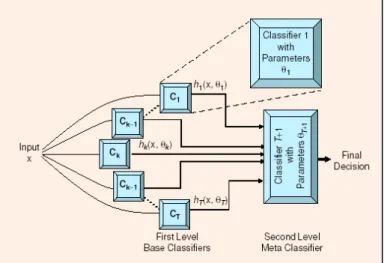
3-1 Mixture of Experts (Polikar, 2006) . . . 69

3-2 The Graphical Representation of Stacked Generalisation Approach (Polikar, 2006) . . . 70

3-3 Behavior Knowledge Space Illustration (Polikar, 2006) . . . 77 3-4 General Architecture for SVM Ensemble (Kim, Pang, Je, Kim, & Bang,

(15)

4-1 Concentrations of CO Data Skewness . . . 111

4-2 Concentrations of CO Data Statistics . . . 112

4-3 SM Method Confusion Matrix AdaBoostM1 Algorithm . . . 117

4-4 SM Method Confusion Matrix Bagging Algorithm . . . 118

4-5 MDNP Method Confusion Matrix AdaBoostM1 Algorithm . . . 118

4-6 MDNP Method Confusion Matrix Bagging Algorithm . . . 119

4-7 MNP Method Confusion Matrix AdaBoostM1 Algorithm . . . 119

4-8 MNP Method Confusion Matrix Bagging Algorithm . . . 120

4-9 LI Method Confusion Matrix AdaboostM1 Algorithm . . . 120

4-10 LI Method Confusion Matrix Bagging Algorithm . . . 121

4-11 LTP Method Confusion Matrix AdaboostM1 Algorithm . . . 121

4-12 LTP Method Confusion Matrix AdaboostM1 Algorithm . . . 122

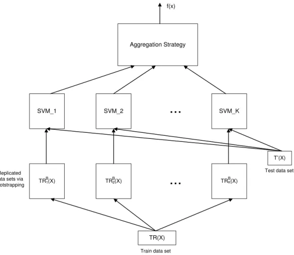
5-1 Illustration of Proposed Decentralised Solution for Spatio-temporal Air Pollution Analysis . . . 126

5-2 Design of Distributed Scalable SVM Ensemble Method (SSELM) for Spatio-temporal Air Pollution Analysis . . . 127

5-3 Updating of SVM Ensemble in SSELM . . . 128

5-4 Illustration of Subsampling Air Pollution Region’s Data via BLB . . . 130

5-5 Subsampling of SSELM on Air Pollution Region’s Data . . . 130

5-6 Training SVM Ensemble via Boosting . . . 131

5-7 Combining Local SVMs Decisions via Weighted Majority Voting Method132 5-8 Illustration of SVM Ensemble for Global Model Decision . . . 134

5-9 SSELM Model vs SVM Ensemble Model Performance on Missing Data 148 5-10 SVM Ensemble Model vs SSELM Model Eﬃciency Comparison on Missing Data . . . 149

5-11 SSELM Model vs SVM Ensemble Model Performance on Training Data 152 5-12 SVM Ensemble Model vs SSELM Model Eﬃciency Comparison on Training Data . . . 153

(16)

5-14 SVM Ensemble Model vs SSELM Model Eﬃciency Comparison on

(17)

List of Tables

3.1 Comparison of Methods . . . 74

3.2 Air Pollution Data Attributes . . . 98

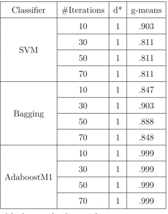
3.3 G-means Metric Results on Spatio-temporal Air Pollution Data . . . 100

3.4 Classiﬁcation Using the SMO . . . 101

3.5 Classiﬁcation Using the Bagging . . . 102

3.6 Classiﬁcation Using the Boosting . . . 102

4.1 Characteristics of CO data . . . 110

4.2 Mean Absolute Errors with SM Method . . . 114

4.3 Mean Absolute Errors with MNP Method . . . 115

4.4 Mean Absolute Errors with MDNP Method . . . 115

4.5 Mean Absolute Errors with LI Method . . . 116

4.6 Mean Absolute Errors with LTP Method . . . 116

5.1 Air Monitoring Sites in the Auckland Region (as of April 2010) . . . 140

5.2 CO Concentrations and Representations . . . 141

5.3 NO2 Concentrations and Representations . . . 142

5.4 O3 Concentrations and Representations . . . 142

5.5 SVM Ensemble Model Performance on Missing Data . . . 145

5.6 SSELM Performance on Missing Data . . . 145

5.7 SVM Ensemble Model and SSELM Model Eﬃciency Comparison on Missing Data . . . 148

5.8 Imputation of Missing Data with Series Mean Method (SMM) . . . . 149

(18)

5.10 SSELM Model Performance on Training Data . . . 151

5.11 SVM Ensemble Model vs SSELM Model Eﬃciency Comparison on Training Data . . . 153

5.12 SVM Ensemble Model Performance on Testing Data . . . 154 5.13 SSELM Model Performance on Testing Data . . . 154

5.14 SVM Ensemble Model vs SSELM Model Eﬃciency Comparison on

Testing Data . . . 155 5.15 Overall SSELM Model Performance . . . 158

(19)

Chapter 1 Introduction

1.1 Background

We need fresh air for our survival and it is vital to our lives. However, our environ-ment is composed of water, earth and space. In the absence of pollution, it would

have been a clean and pleasant place to live in. However, this is now not the case. Our environment is complex and composed of various pollutants that contribute to

its pollution. Environmental pollution can take the form of chemical pollution, waste and water pollution, air pollution, noise pollution, soil and radioactive contamination

or thermal pollution (Bert & Wolterbeek, 2002). The pollution concept is vast, and solutions to every kind of pollution have their own importance. Amongst the various

types of pollution, air pollution is considered to be the most important one (S. A. & Ritz, 2010; R. A. & Becker, 2005; Wuytack et al., 2011) to investigate. People are

more sensitive to air pollution than other forms of pollution (Bell, Morgenstern, & Harrington, 2011; Bernstein et al., 2004; Makri & Stilianakis, 2008). Nowadays,

ev-eryone believes that one can live without food for days and survive for hours without water, but one cannot last for more than a few minutes without air. Hence,

consider-ing the importance and sensitivity of air pollution to mankind, it is the focus of this research to solve the air pollution problem computationally.

Today’s environment is quite diﬀerent from that of the past (Daly & Zannetti, 2007). Population growth and modernisation have increased air pollution over the

(20)

years. Vehicles, industries and urbanisation are considered to be the major factors

responsible for air pollution. Mines, steel factories, cement factories, thermal power plants and reﬁneries are industries that emit a signiﬁcant amount of pollution into

the air (Cole, Elliott, & Shimamoto, 2005). However, our task in the current en-vironment is to improve our air quality and not spreading air pollution. Better air

quality involves the development of suitable control measures either through chemical

or computational studies. Due to the limitations of chemical studies to resolve air pollution problems (State, Popescu, & Gheboianu, 2009), computational studies are

considered to be an eﬀective alternative technique to solve the air pollution problem. It is not a static problem, and doesn’t relate to a particular location. It is dynamic

in nature, changes from location to location, day to day and from hour to hour. Con-ducting a study on air pollution and disregarding this aspect would certainly limit

the results of that study.

1.1.1 Air Pollution

Air pollution is highly topical nowadays, as people know the importance of good air quality on human health (Gosden, MacGowan, & Bannister, 1998). It is considered

to be a burning problem that requires immediate action to control (L. Wang et al., 2010). However, deﬁning pollution is not easy (Vaz & Ferreira, 2009). One can say

that air pollution started when humans started to burn fuels. Man-made emissions through combustion, construction, mining, agriculture and warfare are considered to

be the key contributors to air pollution in today’s environment (Linder, Marko, & Sexton, 2008), as they change the chemical composition of the natural environment.

The common gaseous pollutants of carbon dioxide (CO2), sulphur dioxide (SO2),

nitrogen oxide (NO2) and methane (CH4) can be considered air pollutants in this

context. Hence, we can say that man-made air pollutants are harmful and dangerous for living beings.

However, the above approach has some limitations (Daly & Zannetti, 2007). First of all, we need to deﬁne what harmful means. It could have two meanings adverse

(21)

air’s visibility. Similarly a chemical that is emitted into the air may cause short-term

harmful effects that accrue and create long-term harmful effects. For example (Daly & Zannetti, 2007), man-made emissions of chlorofluorocarbons were not considered

to be harmful as they are static in the lower part of the atmosphere, which is called troposphere. However, with the passage of time it was found that when these

chemi-cals enter the stratosphere, they are converted into a highly reactive species through

ultraviolet radiation. This has a negative eﬀect on the stratospheric ozone. Similarly, carbon dioxide (Qiao, Zhang, Binner, Xu, & Li, 2010) emissions in the air through

combustion processes were considered in the past to be harmless because they were not toxic, but later on researchers found that the long-term accumulation of carbon

dioxide into the atmosphere results in climate change, which could be harmful to our ecosystem.

So besides man-made pollutants through combustion, construction, mining, agri-culture and warfare, it is a good idea to consider air pollution through the non-living

and living world perspectives as well. Air pollution through the non-living world is known as geogenic emissions (Neal et al., 2011), such as volcanic emissions, natural

ﬁres and sea salt emissions, but air pollution through the living world is known as biogenic emissions (Sartelet, Couvidat, Seigneur, & Roustan, 2012). These emissions

come through the living world in forms such as volatile organic compound emissions from forests.

So air pollutants can be deﬁned as any substance emitted into the air from a man-made, geogenic or biogenic source which is not part of the natural

environ-ment or present in higher concentrations in the natural environenviron-ment than speciﬁed (Roberts & Martin, 2006; Cairncross, John, & Zunckel, 2007). In order to address

the air pollution problem, it is worth considering its geogenic and biogenic sources as well. However, man-made pollutants through combustion, construction, mining,

agriculture and warfare are considered to be the main contributors to air pollution in today’s environment (Kawamoto et al., 2011), which have severe health eﬀects on

humans (Leitte et al., 2009; C. & Henry, 2008).

(22)

de-tection that could facilitate strategic decision making for environmental prode-tection,

reduction of damage to ecosystems and protection of human health. However, en-vironmental problems are often complex, and there are many uncontrollable factors

that must be considered when formulating computational analysis. The introduction into the ecosystem of new pollutants can often exacerbate the problem.

Environmen-tal pollution can take the form of chemical pollution, waste and water pollution, air

pollution, noise pollution, soil and radioactive contamination, or thermal pollution (Bert & Wolterbeek, 2002), it is believed that people are normally more sensitive to

air pollution than other forms of pollution (Bell et al., 2011; Bernstein et al., 2004; Makri & Stilianakis, 2008; S. A. & Ritz, 2010; R. A. & Becker, 2005; Wuytack et al.,

2011). Thus air pollution is seen as the ﬁrst priority in the proposed research.

1.1.2 Current Challenges

Environmental problems are spatio-temporal problems, due to the continuously chang-ing environmental conditions resultchang-ing in the movement of pollutants and pollutant

sources. The large volume of spatio-temporal air pollution data from multiple lo-cations comes with signiﬁcant design challenges. This has attracted great deal of

research interest. However, these challenges pose problems for scholars. We will now discuss these challenges.

1. One problem when dealing with large volumes of data are the dynamic nature of big data. Air pollution data consist of huge images and long-term periodic

data continuously captured and stored. This becomes diﬃcult to manage. We also have to deal with the merger of information from asynchronous and varying

distribution networks of sensors, given that sensors are distributed in diﬀerent places.

2. The problem of asynchronous data capture aﬀects the quality and reliability of

the data measures. This problem is exacerbated by the eﬀects of diﬀerent spatial topologies as well as changing macro and micro environmental conditions. To

(23)

19 monitoring stations (which poses spatial problems and macro/micro climatic

problems) day and night (time problem) where data are dynamic (a data vol-ume problem), and if one machine requires maintenance, then data could be

lost easily (a reliability measurement problem and a missing data problem).

3. Often case studies describe solutions to problems where images are of varying sizes or quality, or have minimal or quite varying quality and quantity of

his-torical records. Often, environmental agencies are interested only in the areas which have the highest density of population or are known pollutant producers.

For instance, in New Zealand, the environmental agency puts more eﬀort into understanding the Auckland Environment (highest population) than Hamilton

(4th highest population) data as of June 2013. These studies are often overly restrictive and therefore not useful for a broader understanding of the issues.

4. Often the equipment itself imposes restrictions on the data that can be captured and therefore the types of research activities that can be employed. In an ideal

world, we could install the most useful sensor arrays to capture the data for use with cutting edge computation analysis techniques. Another problem is

that often measuring arrays have been placed in locations that remain static and therefore do not fulﬁll the need to provide real-time data. This forces

the computational analyst to use various algorithms and predictive methods to utilise this otherwise meaningless data. For example, air pollution varies from

location to location and changes over time. It is considered to be dynamic in nature rather than a static dilemma. Because it needs to be addressed from a

spatial and temporal perspective, we make up the inadequacies of data capture with algorithmically complex algorithms and methods.

As a result of challenges of this study, we propose a decentralised and generalised solution so that future researchers can have a solid knowledge base on which to build

their computational analysis studies. We will test our decentralised solution using a case study of computational air pollution analysis. The air pollution in this research

(24)

through a source, whereas the concentration is the amount of pollutant gas present

in the air at a certain location at certain time. We will now discuss some problems in centralised computing and why the decentralised solution is important.

1.2 Problems of Centralised Computing

Traditionally in centralised computing we set up monitoring stations that monitor

our environment through various sensor devices which then transfer the data to one powerful centralised computer to conduct analysis, and based on that analysis,

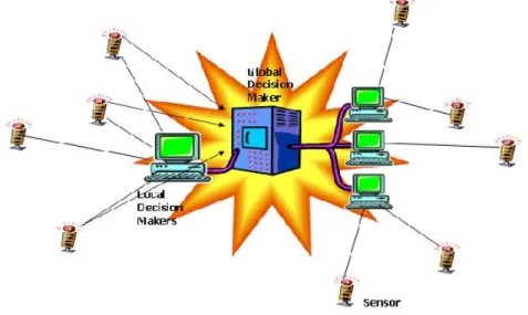
pre-dictions for air pollution are made. Fig 1-1 (Varshney & Mohan, 2005) illustrates a traditional centralised computing solution. However, there are certain complications

associated with centralised computing as detailed below. Combined multiple

moni-Figure 1-1: Illustrated Traditional Centralised Computing Solution (Varshney & Mo-han, 2005)

toring stations’ knowledge, computing and resources are distributed and cannot and should not be centralised for a variety of reasons such as security, load balancing, etc.

Since systems receive huge amounts of asynchronous data, the scale of data can be-come a big data problem. Not only this, but the problem is exacerbated when having

(25)

topical areas for researchers. One of the biggest failures of centralised computing is

its ability to accommodate large amount of data. Traditionally centralised systems were designed to accommodate a certain amount of data, and an increase in the size

of data from the speciﬁed limit results in failure of operation. Often this means data are disregarded or the equipment itself malfunctions.

1.3 Proposed Method

The aim of this study is to propose a generalised decentralised computation solution.

In order to address the problem of decentralised computing, we propose a general framework of SVM Aggregation Modelling for spatio-temporal Air Pollution Analysis.

The main innovations of this work are described below:

1.3.1 Spatio-temporal Analysis

Diﬀerent from the majority of air pollution studies and methods proposed in the

past, spatio-temporal air pollution analysis via SVM aggregation will be conducted. Data partition based on spatio-temporal air pollution analysis through a subsampling

process will maximise the accuracy of the SVM ensemble.

1.3.2 SVM Ensemble for Decentralised Computing

Traditionally air pollution data are distributed across multiple monitoring stations

when this SVM ensemble of decentralised computing approach is deployed. A re-gion’s data chunk is subsampled via an intelligent computation technique. An SVM

ensemble is created on each monitoring station, and their knowledge is transferred to the area’s center. Finally various local decision models are aggregated for a global

decision of air pollution quality. Previous computation techniques proposed for dis-tributed techniques required partial (or fully) oﬄine processing and therefore were

time consuming. The proposed online scalable SVM ensemble learning approach re-sults in a system that has the capability of accommodating real-time data and could

(26)

lead to real-time decision support systems for environmental problem solving.

1.4 Research Questions

The key questions for undertaking this research along with the particular method are

as follows:

1. Dealing with long term historical data of spatio-temporal is always challenging.

SVM ensemble and other methods are used to handle long term historical data, but these methods result in slow processing and low accuracy especially as the

data size increases. Can the data be eﬃciently processed and the accuracy of the model be increased for large data compared to SVM ensemble method? Air

pollution data are available in huge size which need to be stored and processed. The problem is compounded with processing long-term historical data. The

meaning of the data can change over time based on events, and based on the locations from which the data were captured. Dealing with such long term

spatio-temporal data are indeed a challenging assignment.

2. Air pollution is a spatio-temporal problem and the data is distributed across

multiple locations, which is diﬃcult to manage for the SVM ensemble and other techniques. How the distributed nature of spatio-temporal air pollution data

can be resolved eﬃciently and with better classiﬁcation compared to SVM en-semble method? Air pollution data are physically distributed, decentralised

and monitored across various monitoring stations. For example, in the Auck-land region for air pollution monitoring there are 19 monitoring stations. One

can design a computational system for analysing a single air pollution monitor-ing station’s data, but designmonitor-ing a system for processmonitor-ing distributed multiple

data of all those stations is a complex task, since data are available in huge vol-umes. However, centralised data analysis will lead to processing and resource

challenges.

(27)

with such data will not give us the true picture of the fundamental problem.

How accurate can be the analysis of air pollution data with missing values compared to SVM ensemble method? As air pollution varies regionally, it is

comparatively easy to know and compute a single location of air pollution data, but it is diﬃcult to have air pollution regional data based on the computation

of various monitoring stations. Region speciﬁc information will be useful to

formulate a data aggregation strategy.

4. Can SVM aggregation and knowledge fusion over spatio-temporal dimensions be applied to conduct air pollution prediction accuracy better than SVM ensemble

method? Analysis of the results of long-term historic spatio-temporal data are a tedious and time consuming task. Spatio-temporal dimensions fusion via the

same SVM representation is achievable, but still remains a complex task so therefore warrants a speciﬁc research question. We envisage this question to be

more focused on prediction, and any solutions to this research question will be signiﬁcant.

1.5 Thesis Contribution

This thesis mainly proposes a decentralised Scalable SVM Ensemble Learning Method

(SSELM) for classifying spatio-temporal air pollution data in Auckland 2010, which was collected on an hourly basis from 20 monitoring stations. Various SVM ensemble

learning approaches for construction of the ensemble are studied, and these helped in designing the SSELM model and applied on the data. Environmental studies,

specially of air pollution data, are often confronted with missing data. In this regard the performance of various existing imputations methods were studied for imputation

of missing data in the SVM ensemble model construction. The experimental results of the proposed SSELM model outperformed the SVM ensemble model results in

eﬃciency and accuracy.

The proposed decentralised computational solution is a new computational

(28)

spatio-temporal nature of air pollution. The proposed work will lead to a couple of

international conference paper publications (see list of publications). The focus of our research publication has been on diﬀerent aspects of the SVM ensemble learning

methods. The common theme of all the research publications is ensemble learning performance and classiﬁcation accuracies. These research publications are a step by

step guide towards ensemble creation, decision making and its performance analysis.

Following on from above, the aim of this research undertaking is to bring all prior air pollution computational analysis into one cohesive thesis. This thesis will be

beneﬁcial for environmental monitoring authorities for future air pollution prediction. As stated above, the air pollution problem is not a static problem due to its dynamic

nature. A decentralised solution will result in informed decisions via the knowledge fusion of a whole region.

1.6 Thesis Organisation

This thesis is organised as follows: Chapter 2 discusses the historical perspective of air pollution and forms a systematic review of computational air pollution studies

including detection, examination, and prediction. Chapter 3 provides a technical review of SVM based ensemble learning methods, and further in this chapter the

SVM ensemble based learning approach for spatio-temporal air pollution analysis is applied. Chapter 4 discusses the performance of various imputation methods in SVM

ensemble creation. Chapter 5 provides the proposed method scalable SVM ensemble learning method (SSELM) for spatio-temporal air pollution analysis in the Auckland

region along with a critical analysis. Finally, chapter 6 presents our conclusions to this thesis and discusses research contributions.

(29)

Chapter 2 A Review of Computational Air

Pollution Analysis

2.1 Introduction

Computational analysis of air pollution is one way of assisting decision makers in

their approaches to addressing the air pollution problem. Extensive literature on air pollution analysis shows that the measurements used to address and control air

pollution analysis were too conventional and showed the indirect damage caused by it (Vlachokostas et al., 2009). In the past, more importance was given to qualitative

studies compared with quantitative studies (Nakajima, Ozaki, Hongyo, Narama, & Todo, 2011). In contrast, it is true that in quantitative studies we get the extensive

data and documentation on pollutants that aﬀect human health, animal health and plant life. Similarly, environmental statistics identify highly polluted areas or zones,

but the air pollution in such zones or regions shown in pictures is based on simple tests, and such tests are selected based on less or more interpretation of a speciﬁc

eﬀect of air pollution. On the other hand, physical and chemical studies were also conducted in the past for investigation of air pollution analysis; however, substantial

importance should be given to computational environmental studies.

Development of new technologies and increased market competition led to new

(30)

(Goodman, Wilkinson, Staﬀord, & Tonne, 2011). Similarly, there is a constant

in-crease in demand in the ﬁeld of air pollution analysis for better understanding of how to control the levels of air pollutants. Acceptable levels of air pollution and its

eﬀect on human and animal health demand that new research techniques be devel-oped. Hence, our purpose in this research is to develop a computational technique

that provides air pollution analysis of air quality for the future. In our view, such a

technique will certainly beneﬁt human health, animal life and plant growth.

Computational environmental analysis uses techniques from computer science and

applied mathematics to stimulate and analyse computational models of environmental problems. Statistical analysis and machine learning methods have been widely applied

in environmental analysis due to their advantages of fast and eﬀective calculation (Tuia, Ratle, Lasaponara, Telesca, & Kanevski, 2008; Banerjee, Singh, & Srivastava,

2011; Janes, Sheppard, & Shepherd, 2008). Therefore, computational environmental studies provide one of the solutions to deal with environmental problems.

The remainder of this chapter is organised as follows: Section 2.2 discusses the historical perspective of air pollution and describes pollutant emissions in the

Auck-land region. Section 2.3 provides a review of previous computational air pollution detection studies. Section 2.4 presents a review of previous computational air

pollu-tion examinapollu-tion studies. Secpollu-tion 2.5 provides a review of earlier computapollu-tional air pollution prediction studies. Section 2.6 is devoted to limitations of previous

com-putational air pollution studies. Section 2.8 brieﬂy discusses traditional centralised computing. Section 2.9 focuses on research gaps. Finally, section 2.10 presents our

summary for this chapter.

2.2 Air Pollution Data

An air pollutant is a substance in the air that can have adverse eﬀects on humans

and the ecosystem. Air pollution data details concentrations of air pollutants present in the atmosphere. Concentrations of air pollutants have severe eﬀects on human

(31)

in the atmosphere such as sulphur dioxides, nitrogen dioxides, carbon mono oxide,

particulates, ammonia and volatile organic compounds which aﬀect human health. Air pollution data are generally represented as a data stream, as a satellite image or

in spatio-temporal form. These are explained brieﬂy below.

2.2.1 Data Stream

One form of environmental information is the data stream (Medioni, Cohen, Bremond, Hongeng, & Nevatia, 2001). In a data stream the quantity of data are unbounded,

and the speciﬁed atmospheric pollutant concentrations are recorded continuously. The data stream consists of information sourced from environmental parameters that

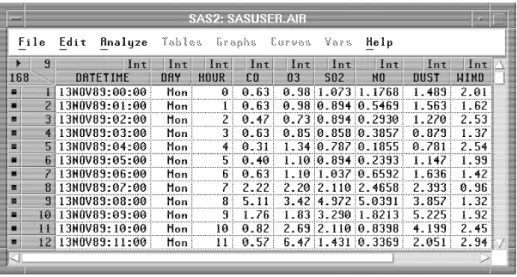
change over time (a time series). For example, air/water quality data represents the pollutants’ concentrations measures. Figure 2-1 (A et al., 1987) shows the

tempo-ral air quality data stream and concentration values of various pollutants, including carbon monoxide, ozone, nitrogen oxide, dust, and other environmental measures for

example wind speed.

Figure 2-1: Temporal Air Quality Data Stream and Concentrations Values of Various

(32)

2.2.2 Satellite Image

Satellite images enable the monitoring of pollutants using various wavelength sensors, allowing the creation of environmental data matrices. Figure 2-2 (Buis & Hosansky,

2012) shows the satellite image, where the associated red intensity levels correspond to regional distribution of greenhouse gases (deduced from temperature variations).

Figure 2-2: Satellite Image (Buis & Hosansky, 2012)

2.2.3 Spatio-temporal Data

Spatio-temporal means data can be either spatial or temporal or both (Grunfeld, 2005).Spatio-temporal data matrices are gaining popularity as a new form of

environ-mental data representation. Such complexity usually results from the environenviron-mental data which contains information on locations, time and states of the environmental

condition (i.e., pollution level). Figure 2-3 (Andrews, 2009) shows the spatio-temporal data of cities and their corresponding years to national Air Pollution Index (API)

(33)

standards. API is collected from several sets of air pollution data and represents the

air quality of a region.

Figure 2-3: Spatio-temporal Data of Cities and Their Corresponding Years to

Na-tional API Standards (Andrews, 2009)

2.3 Historical Perspective of Air Pollution

Air pollution has been a major concern since historical times and is considered to be a threat to human lives (Parr, Stone, & Zeisler, 1996; Jes & Fenger, 2009). Some

laws were introduced at the beginning of 1306 year to prevent air pollution (Jes & Fenger, 2009). During that year Edward I of England banned the burning of sea coal

(34)

Elizabeth I banned the burning of coal in London (Jes & Fenger, 2009). In a sense it

was the industrial revolution that gave birth to an area of air pollution (Cole et al., 2005). An increase in the number of factories and consumption of large quantity of

coal and fossil fuels resulted in extraordinary air pollution.

Air pollution became a major issue after World War II because of atomic warfare,

and its testing created a radioactive spread which is a threat to mankind. Then later

on the tragedy of The Great Smog of 1952 in London killed at least 8000 people (H.R. & Anderson, 2009). All these events have drawn a lot of attention to air pollution

legislation, and this was behind the implementation of The Clean Air Act of 1956 (H.R. & Anderson, 2009).

In the 1970s, President Nixon of the United States formed the Environment Pro-tection Agency (EPA). The formation of the EPA established air quality standards,

and there was a dramatic change in national policy regarding the control of air pol-lution. The main purpose of the air quality standards was to protect the general

health of the public, especially of sensitive populations such as children, older peo-ple and peopeo-ple with asthma (Daly & Zannetti, 2007). The problem of air pollution

was detected late as it cannot usually be recognised as instantly as water pollution. However, in the past the air pollution problem was ignored and was dealt with only

when it became a health threat to the mankind (Triolo, Binazzi, & Cagnetti, 2008). To explore the air pollution problem historically, we will look at some of the

trends in air pollution over the years in the Auckland region. The common gaseous pollutants investigated for our research are Sulphur dioxide, Nitrogen oxide,

Car-bon monoxide, Particulate matter and Ozone. As we know that the air pollution has adverse eﬀects on our environment and health (Makri & Stilianakis, 2008). The

Auckland Council is monitoring concentrations of gaseous pollutants such as Sulphur dioxide, Nitrogen oxide, Carbon monoxide, Particulate matter and Ozone at various

sites. These pollutants have negative eﬀects on public health and especially on peo-ple who have respiratory problems (Leitte et al., 2009). For the year ending 2005,

measurements taken by Auckland Council show that there is an increase in vehicle emissions of Carbon monoxide (Council, 2010) and that levels of Nitrogen oxide and

(35)

Carbon dioxide have exceeded the standard levels for the year ending on March 2005

(Council, 2010).

The levels of gaseous pollutants such as Sulphur dioxide, Nitrogen oxide, Carbon

monoxide, particulate matter and ozone emissions over the years in the Auckland Region are investigated in this chapter. This will indicate how serious the air pollution

problem is.

2.3.1 Sulphur Dioxide Emissions into the Air from

1977

to

2009

The data in Figure 2-4 shows the sulphur dioxide emissions into the air from 1977 to 2009. This data has been collected from a site in Penrose, Auckland. The decrease

in emissions of sulphur dioxide in the air from the 70s and 80s is due to a decline in the use of coal in industries. But the level of sulphur dioxide in emissions is on the

rise due to an increase in the number of diesel vehicles.

(36)

2.3.2 Nitrogen Oxide Emissions into the Air from

1989

to

2009

The data in Figure 2-5 shows the nitrogen oxide emissions into the air from 1989 to 2009. This data has been collected from monitoring sites across the Auckland region

at Khyber Pass Road, Takapuna, Queen Street II, Glen Eden, Penrose, Musick Point, Henderson, Kingsland, Mt Eden and Patumahoe over the years. The increase in the

concentrations of nitrogen oxide in the air is due to increase in numbers of vehicles on the road. However, nitrogen oxide emissions at urban monitoring sites were 66%

less than the National Environmental Standards in that particular region, but those concentration levels still exceed standards along roadside monitoring sites.

Figure 2-5: Nitrogen Oxide Emissions into the Air from 1989 to 2009 (Council, 2010)

2.3.3 Carbon Monoxide Emissions into the Air from

1991

to

2009

The data in Figure 2-6 shows the carbon monoxide emissions into the air from 1991 to 2009. This data wa collected from monitoring sites at Queen Street II and III,

(37)

Carbon monoxide emissions into the air have dropped signiﬁcantly over recent years,

but the concentration level in the air might go above the ambient air quality guidelines (Council, 2010). Moreover, the concentration levels of carbon monoxide were recorded

as less than the National Environmental Standards at urban monitoring sites.

Figure 2-6: Carbon Monoxide Emissions into the Air from 1991 to 2009 (Council,

2010)

2.3.4 Particulate Matter Emissions into the Air from

1994

to

2009

The data in Figure 2-7 shows the particulate matter emissions into the air from 1991 to 2009. Particulate matter at level PM10was collected from monitoring sites at Khyber

Pass Road, Queen St, Penrose, Glen Eden, Patumahoe, Botany Downs, Henderson, Kingsland, Takapuna, Kumeu and Pakuranga over the years. The concentration level

of PM10into the air has increased in the last few years and even exceeded the National

(38)

Figure 2-7: Particulate Matter Emissions into the Air from 1991 to 2009 (Council,

2010)

2.3.5 Ozone in the Air from

1997

to

2009

The data in Figure 2-8 shows the ozone in the air from 1997 to 2009. This data

were collected from monitoring sites over the years from Patumahoe, Sky Tower,

Whangaparaoa, Musick point and Kingsland. The ozone emissions levels are very close to the National Environmental Standards at these air quality monitoring sites

(Council, 2010). However, it still requires monitoring authorities to be alert to the ozone concentration in air.

The above historical emissions data on sulphur dioxide, nitrogen oxide, carbon monoxide, particulate matter and ozone shows that the concentration of these gaseous

pollutants into the air was increasing and is still increasing today (Council, 2010). This is not only harmful to our environment but also creates threats to our lives.

However, chemical changes to our environment result in foreseeable and unforeseeable impacts that need to be measured and controlled eﬀectively in order to save lives,

especially of older people and young children, who are at great risk from these air pollutants.

(39)

Figure 2-8: Ozone in the Air from 1997 to 2009 (Council, 2010)

2.4 Computational Air Pollution Detection

Stud-ies

Air pollution detection is used to identify the location and types of pollution in the

environment. Air and environmental pollution detection is a fundamental step to

providing useful information about air pollution examination and prediction.

For ﬁre smoke detection, (Z. Li, Khananian, Fraser, & Cihlar, 2001) studied neural networks to classify a scene into smoke, cloud or clear background, and generated

con-tinuous outputs to represent the mixture portions of these objects. For investigating

oil spills from ships, (Solberg, Storvik, & Solberg, 1999) computed a set of features for each dark spot, and authenticated a spot as either an oil slick or a lookalike. For

detecting and monitoring environmental anomalies and changes, (Carlotto, Lazaroff, & Brennan, 1992) used a spectral classification method to detect specific areas in an

image for anomaly and change detection followed by knowledge-based techniques to identify general categories based on the spectral shape.

(Roadknight, Balls, Mills, & Palmer-Brown, 1997) used principal components analysis (PCA) together with standard multilayer perceptron (MLP) and multiple

(40)

regression analysis for decision support in determining critical levels of ozone

pollu-tion. (Z. Li et al., 2001) developed neural networks and threshold classiﬁer methods to identify potential areas covered by smoke and further used texture analysis and

spatial ﬁltration to remove false classiﬁed pixels. (Gacquer, Delmotte, Delcroix, & Piechowiak, 2006) used cameras and analysed pictures for pollution detection

prob-lems. Visual scenes around complex plants were recorded and various signals were

computed to describe pictures. Bayesian networks and a k-nearest neighbor classiﬁers were used in this study to derive results.

The above computational air pollution detection studies make use of methods such as multilayer perceptron, principal components analysis and threshold classiﬁers. It

is worth noticing that in these studies methods were performed on limited static air pollution data. This is not useful enough as real world air pollution data are presented

as continuous data streams. In order to solve the dynamic distributed nature of air pollution problems, the data ﬁrstly needs to be aggregated and shared from

spatio-temporal perspective. Overlooking the dynamic characteristic of air pollution in any computational methods will not provide us with a complete enough picture for air

pollution analysis. Disregarding the time variation and overlooking location variation for any air pollution detection study will provide only partial results.

2.5 Computational Air Pollution Examination

Stud-ies

Air pollution examination evaluates the level of pollution and the eﬀects of pollutants based on the information provided by the change detection system. It provides the

current state of air pollution to people who are working on pollution control.

In the past, a variety of computational studies have been done to examine the

diﬀerent aspects of air pollution. For smoke, water and forest pollution, (Carlotto et al., 1992) proposed to use Multispectral Imagery (MSI) to monitor environmental

(41)

forest pollution were successfully identiﬁed.

In the decision making on environmental pollution, urban areas play a pivotal role in analysis. To address this along with other proposed methods in the literature,

spa-tial analysis was extended through geostatistical methods along with dynamic models (Matvejivcek, Engst, & JaNour, 2006). In the proposed method spatial analysis

con-sidered the processing of a wide range of water, air and soil pollution data. Further,

data from remote sensing was also considered. Within the framework of geographic in-formation systems, integration and spatial data management were carried out. From

a modeling perspective, a geographic information system was primarily used for the preprocessing and postprocessing of the data that needed to display in digital map

layers and was visualised in 3D scenes. In this research, a geographic information system was mainly used for spatio-temporal analysis, or to create a relationship

be-tween geographical information system databases and stand-alone modeling tools. The proposed approach was helpful for environmental local authorities to print out

environmental protection issues.

To investigate modern trends in monitoring and analysis of environmental

pollu-tants, (Namiesnik, 2001) conducted a study to provide the information required for a reliable evaluation of the state of environment pollution and the changes taking

place. It is noticeable that (Versaci, 2002) studied Sophisticated Fuzzy Interference Systems (FISs) to provide direction for the design of an environmental examination

system to estimate and predict the pollutant values.

The general trend of air pollution examination is that when data are obtained

from a static monitoring station, a computation method is applied for analysis, and results are obtained for examination. It is worth noting that to examine air pollution

and to estimate pollutant values, the above research uses a centralised monitoring station data and determined air pollution status on these results. This is not a true

criterion for air pollution examination. In order to examine air pollution, spatio-temporal analysis is essential because air pollution changes from location to location

and time to time. The choice of monitoring stations is another problem for air pol-lution examination. Not all monitoring stations provide useful information for air

(42)

pollution examination. Aggregating the knowledge of multiple monitoring stations

and applying divide and conquer strategy using an intelligent system will contribute better results for air pollution examination.

2.6 Computational Air Pollution Prediction

Stud-ies

Air pollution prediction simulates the progress and estimates the future trend of

pol-lution. It is based on the current information retrieved by a pollution change detection system. It helps environmental monitoring authorities to construct strategies to deal

with air pollution problems. The common problems faced in pollution prediction are occurrence of special events and missing data.

For predicting air temperatures up to 12 hours ahead, (Smith, McClendon, & Hoogenboom, 2007) collected parameters on air temperature, solar radiation, wind

speed, rainfall and relative humidity and then applied Artiﬁcial Neural Network (ANN) computing to obtain their results. For complicated environmental data

pro-cessing, (Osowski & Garanty, 2006) used Support Vector Machine (SVM) plus wavelet decomposition methods for daily air pollution forecasting on NO2, CO and SO2 dust

pollutants.

Air quality deterioration and its changes to human health attracted various

re-searchers to formulate a model that can make predictions of air quality. However, the limited number of air quality monitoring stations and the complexity of inﬂuencing

factors on air quality resulted in an increase in development of future air quality pre-diction. In this regard, a temporal-spatial aggregated framework was proposed, using

multiple temporal and spatial data sets to predict future air quality (X. Lu, Wang, Huang, Yang, & Shen, 2016). In the proposed framework various factors inﬂuencing

air quality from temporal-spatial perspectives were analysed to formulate a linear regression based inference model. The linear regression model estimated not only the

(43)

data for the model to predict air quality for the future. The proposed model

pro-vided superior parameters for learning and overmatches the existing machine learning approaches.

In the past three decades there has been a rapid growth in the Chinese economy (L. Liu et al., 2016). However, the economic boom resulted in deterioration of the

urban air quality. To address this the air pollution burden and its association with

cli-matic factors along with health outcomes was analysed (L. Liu et al., 2016). Multiple linear regression models, panel ﬁx models and spatial autocorrelation were conducted

in association with climate factors. Sensitivity analysis was conducted by considering the time-lag eﬀect between exposures and outcomes. The study concluded that air

pollution varied by season and regions and correlated with climate factors.

A methodology for spatio-temporal interpolation of air quality data were proposed

(Romanowicz, Young, Brown, & Diggle, 2006). Spatio-temporal variability of obser-vations of nitrogen oxide was divided into time-series analysis of available data and

the development of combined spatio-temporal using nitrogen oxide observations. The results of this study indicated that the sample spatio-temporal model consisted of

trend and noise eﬃciently, showing the spatio-temporal variations in the data which can easily be applied to the un-sampled locations to predict air pollution variations

in time and space.

An ensemble forecasting approach to forecast maps on a daily basis for air

pol-lutants ozone, nitrogen oxide and particulate matter was proposed (Debry & Mallet, 2014). This approach relied on multiple air quality models. These air quality models

were diﬀerent in parameterisations, input and numerical strategies. So, one model may perform better with respect to observations for an examined pollutant at a

cer-tain time and location. The results of this study indicated that errors in forecasting were reduced hourly, daily and during peak concentrations.

Air quality forecasting in urban areas is quite diﬃcult because of the uncertainties in describing metrological and emission factors. To enhance forecasting accuracy, a

hybrid artiﬁcial neural network and a hybrid support vector machine (P. Wang, Liu, Qin, & Zhang, 2015) were used. Firstly, an artiﬁcial neural network along with a

(44)

forecasting system was applied on the historical data. Then the residual information

of the error was used to revise the forecasting target by deploying the Taylor expansion forecasting method. The novelty in the proposed method was that it successfully

used residual information on an incomplete input variable condition that enhanced the forecasting accuracy of the model.

To investigate the concentration of particular matter, a hierarchical spatio-temporal

model (Cameletti, Lindgren, Simpson, & Rue, 2013) was proposed. The model con-sisted of Gaussian ﬁeld, which was inﬂuenced by measurement error and a state

process known by a ﬁrst order autoregressive model. The main objective of the re-search was to present an eﬀective estimation and spatial prediction strategy for the

spatio-temporal model.

Using a time series prediction of air pollution, (Castro, Castillo, Melin, &

Rodriguez-Diaz, 2008) applied an Interval Type-2 Fuzzy Neural Network (IT2FNN) hybrid method to predict the impact of meteorological pollutants such as O3 over an

ur-ban area. (Zito, Chen, & Bell, 2008) used several Neural Networks (NNs), such as multilayer perceptron (MLP), radial basis function (RBF) and modular network

(MN) to estimate real-time roadside CO and NO2 concentrations. (Ando, Graziani,

& Pitrone, 2000) proposed a ‘black box’approach consisting of linear, nonlinear and

neural network models, for air pollution modelling, where air pollution concentration is predicted as a function of the expected causes, based on meteorological forecasts.

(Huang, Zhou, Ding, & Zhang, 2012a) used the O3 attribute to predict air quality

in the future, and deployed an order weight average (OWA) based time series model.

(Zheng, Yu, & Yu, 2012) deployed a Response Surface Methodology (RSM) to pre-dict NOx emissions. The predicted NOx emissions were compared with standard

measures and had a relative error rate of less than 5%. Further, the RSM model was simpler than the non-analytic models such as generalised regression neural network

and support vector regression.

Perhaps the earlier work on computational air pollution prediction was started in

the early 20th century. In the 1980s a Group Method of Data Handling (GMDH) algorithm was proposed (Tamura & Kondo, 1980). This algorithm had the

(45)

abil-ity not to divide the available data into training and testing data for determining

the structure of the partial polynomials or determining the number of intermediate variables. The GMDH algorithm was applied for the short term prediction of air

pol-lution concentrations. For this study SO2 time series data were deployed. Based on

the wind velocity and wind direction in Tokushima in Japan a few hours advance SO2

was developed. The results obtained were compared with a linear regression model

and linear autoregressive model where the GMDH algorithm outperformed the other models.

As most of the country population is urban their activities from one place to another result in air pollution in urban areas. In this regard a system for monitoring

and forecasting air pollution in urban areas was proposed (Shaban, Kadri, & Rezk, 2016). The proposed system deployed low-cost-air quality monitoring motes that

were easily available through an array of gaseous and meteorological sensors. These motes were then transferred to an intelligent sensing platform which consisted of

several modules. These modules were responsible for receiving and storage of data and further converting the data into useful information for forecasting the pollutants.

Three machine learning algorithms such as support vector machines (SVM), artiﬁcial neural network (ANN) and M5P model trees were deployed. The results depicted that

multivariate modeling with M5P algorithm provided the best forecasting accuracy for SO2 other to other algorithms.

Nitrogen oxide emission from vehicles emission results in considerable health is-sues. In this regard an accurate online support vector regression model (AOVSR) was

proposed for the emission prediction of nitrogen oxide (NOx) (J. Zhou, Ji, Qiao, Si, &

Xu, 2013). It was evident from the results that AOVSR performance on small sample

data were quite eﬃcient in comparison with the support vector regression model and artiﬁcial neural network. The proposed model had the capability to predict NOx

emission accurately under certain conditions when parameters were modiﬁed. The overall eﬃciency and prediction accuracy of the proposed model was enhanced as it

had the ability to update the parameters by itself with respect to change in time and change of other parameters.

(46)

Particulate matter PM is consists of solid and liquid particles which remain in the

air for a while, creating a great threat to human health. This provides an opportunity for the researchers to consider the causes of PM emission, depending of its level of

concentration in the air at a certain time and place. Hence, a method for PM emis-sion prediction based on least a square support vector machine (LS-SVM) algorithm

was proposed (Z. H. Li & Yang, 2010). The LS-SVM algorithm was based on the

principle of reconstruct phase space which was derived from the Takens Embedding Theorem. In this method, the data were divided into two parts, training and testing.

The learning model was obtained by window moving having width n, along the axis time. The results of LS-SVM demonstrated better predication of PM2.5 by numerical

experiments.

The fast growth of industrial activities has resulted in an air pollution problem,

which is a major concern for public health. An innovative wireless sensor network for air pollution monitoring system (WAPMS) has been proposed (Khedo, Perseedoss, &

Mungur, 2010). The proposed system makes use of an air quality index for air pollu-tion monitoring in Mauritius. To improve the eﬃciency of WAPMS a new algorithm

for data aggregation named Recursive Quartiles (RCQ) was implemented. This new algorithm RCQ had the ability to eliminate duplicate and invalid readings, which

resulted in reduction of data transmission to a centralised station. To handle any privacy and management issues WAPMS was equipped with a hierarchical routing

protocol, which caused the motes to sleep in idle time.

It is very important to know the causes of air pollution to avoid further loss to

humans and other living organisms. In order to ﬁnd out the sources of air pollution, a principal components analysis was deployed (Singh, Gupta, & Rai, 2013). Along with

the PCA tree ensemble based learning were constructed for the prediction of urban air quality. The PCA has identiﬁed that the vehicles emission and fuel combustion

are the main two sources of air pollution. Various tree based ensemble learning i.e., decision tree forest, single decision tree and decision treeboost generalisation

and predictive performance was evaluated and compared with conventional machine learning approaches such as SVM. The miss-classiﬁcation rate for a single decision

(47)

tree was 8.32%, 4.12% for decision tree forest, 5.62% for decision treeboost and 6.18%

for support vector machines. The classiﬁcation accuracy of decision tree forest and decision treeboost ensembles was comparatively high compared with the classiﬁcation

accuracy of SVM classiﬁcation and regression. This was successfully completed by deploying bagging and boosting algorithms with these tree based ensemble models.

As mentioned earlier, incomplete or missing data represents incomplete results.

This is because missing data machine learning algorithms confront the problem of in-accurate prediction performance. In order to handle the missing environmental data

a spatial data aided incremental support vector regression (SalncSVR) model for spatio-temporal PM2.5 was proposed (Song, Pang, Longley, Olivares, & Sarrafzadeh,

2014). In the proposed method, spatial data were used for the training of the tem-poral prediction model. PM2.5 data were obtained through 13 monitoring stations

in Auckland, New Zealand. The results of the SalncSVR model were compared with the temporal lncSVR model, and the SalncSVR model resulted in better prediction

statistics.

Furthermore, some authors have focused their eﬀorts on forecasting air pollution

by machine learning approaches such as neural networks, support vector machines and kernel based algorithms. However, to reduce the error rate between the model

and the raw data, a mixed approach consisting of support vector machines and ker-nel functions was proposed for forecasting urban air quality (Sotomayor Olmedo et

al., 2013). The kernel functions that were considered for pollutants concentration forecasting of PM 2.5, SO2 and O3 were Gaussian, Polynomial and Spline. The

ap-plication of SVM along with these kernels resulted in better accuracy modelling for pollutant concentration forecasting.

In the past, data mining techniques were deployed as well for eﬀective air pollution forecasting. Artiﬁcial neural network models consisting of data mining techniques

based on Feed Forward Neural Networks (FFNN) and Multilayer Perceptron (MLP), and neural network models were applied for urban and industrial air pollution impacts

area (Christy & Khanaa, 2016). The air pollution patterns obtained showed a greater accuracy and lower error rate with the MLP neural network model.

(48)

Traﬃc and environmental data are also presented as a time series. Due to the

dynamic nature of real time-data predicting, improving performance of such a task is a great challenge. With this aim, a new type of ensemble based on a bagging

algo-rithm was proposed to improve the predictive performance of real-time data (Oliveira & Torgo, 2014). Diversity is very important in ensemble creation. In this regard

di-versity was created through bagged regression trees. However, this study focused on

diversity creation through bagging, but it failed to highlight the aggregation strategy of decision making of the various ensemble models.

Lastly, in terms of air pollution daily prediction, a method using support vector machines and wavelet decomposition was proposed (Osowski & Garanty, 2007). The

measured time series data were decomposed into wavelet representation, and from there wavelet coeﬃcients were predicted. From these wavelet coeﬃcient values the

ﬁnal daily air pollution forecast was prepared. The forecast approach was proposed by applying a neural network of SVM type, applying a regression mode. However,

the study of this work was limited to the Gaussian kernel.

However, it is noticeable that the above computational air pollution prediction

studies were isolated pieces of research, based on monthly statistical data and yearly pollution predictions. Made this way they may be scientiﬁcally true but not useful in

practice. Neglecting the spatio-temporal nature of air pollution, and predicting air temperature in advance by collecting parameters on air temperature, solar radiation,

wind speed and relative humidity doesn’t authenticate temperature prediction results. Similarly, conducting time series predictions of air pollution from a temporal

per-spective while disregarding the spatial aspect will give us alarming results. Calcu-lating air pollutants NO2, CO and SO2 concentrations using order weight average

(OWA), response surface methodology (RSM), multilayer perceptron (MLP), radial basis function (RBF) and modular network (MN) methods along with the centralised

data monitoring source overlooking the dynamic, decentralised and streaming nature of air pollution will not help solve the air pollution problem. In contrast, a useful

computational detection system should be capable of spatio-temporal air pollution data analysis and should have the ability to perform knowledge fusion across whole

Support Vector Machine (SVM) aggregation modelling for spatio-temporal air pollution analysis