Portland State University
PDXScholar
Dissertations and Theses Dissertations and Theses
Spring 5-26-2016
Event Detection Using Correlation within Arrays of Streaming
PMU Data
Jordan Landford
Portland State UniversityLet us know how access to this document benefits you.
Follow this and additional works at:http://pdxscholar.library.pdx.edu/open_access_etds Part of thePower and Energy Commons
Recommended Citation
Landford, Jordan, "Event Detection Using Correlation within Arrays of Streaming PMU Data" (2016).Dissertations and Theses.Paper 3031.
Event Detection Using Correlation within Arras of Streaming PMU Data
by Jordan Landford
A thesis submitted in partial fulfillment of the requirements for the degree of
Master of Science in
Electrical and Computer Engineering
Thesis Committee: Robert Bass, Chair Melinda Holtzman
Abstract
This thesis provides a synchrophasor data analysis methodology that leverages both statistical correlation techniques and a statistical distribution in order to identify data inconsistencies,
as well as power system contingencies. This research utilizes archived Phasor Measurement Unit (PMU) data obtained from the Bonneville Power Administration in order to show that this methodology is not only feasible, but extremely useful for power systems monitoring,
decision support, and planning purposes.
By analyzing positive sequence voltage angles between a pair of PMUs at two different substation locations, an historic record of correlation is established. From this record, a
Rayleigh distribution of correlation coefficients is calculated. The statistical parameters of this Rayleigh distribution are used to infer occurrences of power system and data events.
To monitor an entire system, a simple solution would be observing each of these parameters for every PMU combination. One issue with this approach is that correlation of some PMU pairs may be redundant or yield little value to monitoring capabilities.
Additionally, this approach quickly encounters scalability issues as each additional PMU adds considerably to computation - for example, if the system containsnPMUs the amount
To address these issues, an alternative scheme is proposed which involves monitoring only a subset of PMUs characterized by electrically coupled zones, or clusters, of PMUs. These clusters include both electrically-distant and electrically-near PMU sites. When
monitored over an event, these yield statistical parameters sufficient for detecting event occurrences. This clustering scheme can be utilized to significantly decrease computation time and allocation of resources while maintaining optimal system observability.
Results from the statistical methods are presented for a select few case studies for both data and power system event detection. In addition, determination of cluster size and content is discussed in detail. Lastly, the viability of monitoring pertinent statistical parameters over
Dedication
Dedicated to those who have supported and fostered my academic pursuit. These include my mother and her boyfriend, George, for financially supporting me during a majority of my undergraduate years. My common law wife, Mary Grace, for providing me with emotional support, helping me grow as a person, and taking care of me during times of sickness. Lynn Montoya and Sarah Elsasser at the PCC ROOTS organization for helping me figure out a plan early in my academic career. Dr. Melinda Holtzman for playing a large role in assisting me in obtaining the ORBest scholarship. Lastly, my advisor, Dr. Robert Bass, for providing such a great opportunity through this research project, the ORBest scholarship, and through his fantastic power engineering program at the Maseeh College of Engineering and Computer Science.
Acknowledgements
A deep and sincere thank you to Tony Ferris at the Bonneville Power Administration, Johanna Brickman from Oregon BEST, and Rachel Stansbury from the Maseeh College.
Contents
Abstract i
Dedication iii
Acknowledgements iv
List of Tables vii
List of Figures viii
1 Problem Statement 1
2 Literature Review 4
2.1 Intermediate Work . . . 7
3 Background 9 3.1 Synchrophasor IEEE Standard . . . 9
3.1.1 Phasor Definition . . . 10
3.1.2 Timetags and Synchronization . . . 10
3.1.3 Measurement Requirements . . . 11 3.2 Sequence Components . . . 12 3.3 Dataset Characteristics . . . 14 3.4 Network Topology . . . 15 4 Design Methodology 17 4.1 Correlation . . . 17 4.2 Window Length . . . 18 4.3 Correlation Visual . . . 20
4.3.1 Historic Playback Engine . . . 21
4.3.2 Data Structure . . . 22
4.8 Cluster Size . . . 42
4.9 Cluster Content . . . 44
5 Results & Analysis 47 5.1 Detecting Data Errors and Power System Events . . . 49
5.2 Window Length . . . 53
5.3 Rayleigh Characteristics . . . 58
5.4 Cluster Scheme . . . 65
5.4.1 Analyzing Other Events . . . 70
6 Discussion 86
7 Conclusion 89
Bibliography 91
List of Tables
4.1 Negativerentries (in percent) ofφ+ . . . 27
4.2 Negativerentries (in percent) ofV+ . . . 27
4.3 µ(x)ofφ+ . . . 29
4.4 var(x)ofφ+ . . . 29
4.5 Sweep of K values to determine normalizedxexceeding threshold and classified false-positives. . . 35
5.1 Quantifying the change in the spread ofxof the Rayleigh distribution during an event. . . 64
List of Figures
1.1 PMU Interface . . . 2
3.1 Phase and Symmetrical components . . . 13
3.2 System topology . . . 15
4.1 Time domain plot ofV+ andφ+during event . . . 19
4.2 Sample correlation visual . . . 21
4.3 Data structure of correlation visual . . . 22
4.4 Case study PMU cluster . . . 24
4.5 Event detection metric withK = 10 . . . 32
4.6 Event detection metric withK = 100 . . . 33
4.7 Event detection metric withK = 250 . . . 34
4.8 Maximum false-positive threshold values for all PMUs . . . 36
4.9 Maximum true-negative threshold values for all PMUs . . . 37
4.10 Visual structure characterizing data events . . . 39
4.11 Visual structure during an event . . . 41
4.12 Exclude PMUs when MFPTV > MTNTV . . . 42
4.13 Cluster on PMUs with low MFPTV . . . 43
4.14 Time domain plot comparison / impact ofrduring event for all near cluster . . 45
4.15 Time domain plot comparison / impact ofrduring event for all far cluster . . . 46
5.1 Time domain plot comparison / impact ofrduring event for case study cluster . 48 5.2 Impact ofrduring data drop . . . 50
5.3 Impact ofrduring data drift . . . 52
5.4 µ(x)ofφ+13 cycles into a lightning event . . . 54
5.5 var(x)ofφ+13 cycles into a lightning event . . . 55
5.6 Correlation visual ofφ+13 cycles into an event . . . 56
5.7 Comparison ofvar(x)overV+andφ+. . . 59
5.8 Rayleigh distribution of φ+ over 15 cycle window size before/during event occurrence . . . 61
5.9 Rayleigh distribution of φ+ over 30 cycle window size before/during event occurrence . . . 62
5.10 Rayleigh distribution of φ+ over 60 cycle window size before/during event occurrence . . . 63
5.12 Event 1: Normalizedxduring an event . . . 68
5.13 Event 1: Normalizedx40 cycles into an event . . . 69
5.14 Event 2: Time domain response 40 cycles into the event . . . 71
5.15 Time domain response over case study cluster for event 2 . . . 72
5.16 Visual structure 13 cycles into event 2 . . . 73
5.17 Event 2: Normalizedxprior to the event . . . 74
5.18 Event 2: Normalizedx . . . 75
5.19 Visual structure 40 cycles into event 2 . . . 76
5.20 Event 2: Normalizedx40 cycles into the event . . . 77
5.21 Event 3: Time domain response 40 cycles into the event . . . 79
5.22 Time domain response over case study cluster for event 3 . . . 80
5.23 Visual structure 13 cycles into event 3 . . . 81
5.24 Event 3: Normalizedxprior to the event . . . 82
5.25 Event 3: Normalizedxduring the event . . . 83
5.26 Event 3: Normalizedx40 cycles into the event . . . 84
1 Problem Statement
Recently, electrical power grids have experienced an influx of renewable generation sources, flexible and dynamic loads, and increased cybersecurity concerns. Pressure from these
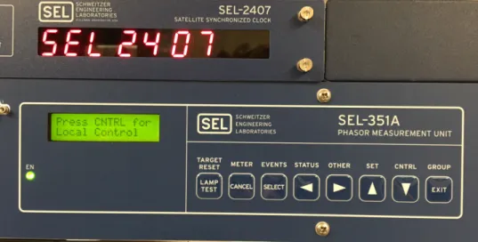
issues places significant emphasis on accurately determining the current state of the grid. To this end, synchrophasor technology, orPhasor Measurement Units (PMUs), provide a viable solution through real-time grid monitoring. Briefly, PMUs are data collecting devices that
capture highly granular, time-stamped phasor measurements of electrical waveforms from electrical power systems. This increased monitoring capability is leading to enhanced levels of observability, grid control, and decision support within grid operation centers. Currently,
however, power operations do not yet rely solely on PMU data; real-time applications, such as state estimators and remedial action schema, currently do not utilize the benefits
of these high fidelity measurements. The analysis method presented in this thesis offers a statistical-based monitoring scheme purposed for real-time detection of both data events and power flow contingencies with the objective of providing increased awareness to grid
Figure 1.1: Actual Phasor Measurement Unit setup in PGE Power Engineering Lab.
Currently, Supervisory Control and Data Acquisition (SCADA) systems serve as the
basis for grid monitoring. SCADA systems sample data every 1 to 4 seconds. Monitoring schema use these data and state estimators to determine power system voltages and power flows. PMU measurements are far superior to SCADA measurements in terms of resolution
and accuracy as measurements can be taken at rates up to 120 phasor measurements per second, neglecting the need for state estimation. The high data measurement rate also provides insight into the transient nature of contingencies.
The methods proposed in this thesis use PMU data for detection of both data errors and power system events. The method is a statistically-based middle-ware algorithm intended to inform higher-level applications of abnormal system behavior. For instance, the algorithm
could inform remedial action schemes that actuate autonomous control over a power system in response to power system events. Integrity of the data must be ensured in order to avoid
a metric for detecting occurrences of power system events at or near real-time. With this in mind, these methods aim to minimize computation time and allocation of computing resources, necessary characteristics to achieving real-time monitoring and control.
In this thesis, a monitoring stratagem based on a PMU site clustering scheme is intro-duced. Clustering schemes such as those described by Pierce, et al., have been shown to be highly informative for retrospective detection of previously unidentified events [1]. In
our work, PMU clustering is done by selecting a ‘sufficient’ amount of PMU data streams to monitor in order to optimize monitoring over a particular area within a system while minimizing computational resources and computation time.
By selecting a subset of PMUs from this area, a cluster containing a combination of both electrically-near and electrically-far PMUs, a pairwise comparison between each PMU site’s positive sequence phase angle is made using a linear statistical method to create a vector of
correlation values. These correlation vectors are then used to define a Rayleigh distribution from which statistical parameters can be quantified. By monitoring clusters of near-far PMU sites and calculating these statistical parameters, metrics for identifying disturbances within
this area of the system are established.
The capability of this clustering method, when used in analyzing pairwise positive
sequence phase angles to determine statistically significant Rayleigh parameters for event detection, is demonstrated. In addition, its robustness in data and power system event detection is demonstrated with a ‘window size’ feature (discussed in detail in Chapter 4.2).
2 Literature Review
Over the past few years, extensive research efforts have been made towards event detec-tion using PMU-generated data. These methods can roughly be categorized as statistical
algorithms or signal processing algorithms.
In regards to the latter, some efforts are based on Principal Component Analysis (PCA), a mathematical procedure that uses an orthogonal transformation to convert a set of
obser-vations of possibly correlated variables into a set of linearly uncorrelated variables called principal components. PCA is a useful statistical technique that is commonly used for finding patterns in data of high dimension. Ge, et al., defined simple rules for voltage and
power event detection at the distribution level where voltage events include sags, swells, under/over voltage, and interruptions and power events include load drops and surges [2].
Conversely, rules can be made complex, as described by Xie, et al., in which they provide a dimensionality reduction analysis at the transmission level in order to significantly lower dimensional “signature” of the states in the overall power system to detect line and unit
tripping [3].
components. Sant, et al., use Prony’s method to characterize line switching and unit tripping for a handful of events [4].
Yet another type of signal processing technique includes a method for determining
the statistical self-affinity of a signal, known as detrended fluctuation analysis (DFA), as discussed by Ashton, et al., in which analysis over system frequency is performed to determine values of fluctuation [5]. These values can then determine line and unit tripping
occurrences.
The most relevant effort that closely resembles the methods proposed in this thesis was developed by Sohn, et al., [6]. This work uses both statistical and signal processing
tech-niques, namely, linear analysis, residual modeling, and short-time Fourier transforms. Based on these methods, parameters, such as mean, variance, and correlation, were determined. For each of these parameters, which they refer to as indices, a set of decision rules are
defined in order to provide indication of an event occurrence.
This work closely resembles the methods covered in this thesis in a few ways. They are conceptually similar in that statistical parameters are determined from statistical methods
and are used to derive metrics for event detection. Additionally, the defined rules provide indication of an event occurrence in a similar fashion; an event will be declared if these
parameters exceed some established threshold value. Another similarity is the challenge of determining an appropriate threshold value.
This work is also different than the methods proposed in this thesis in a few ways. First,
are different; while this work does not explicitly state the statistical methods, it is assumed that they are not the same. Lastly, this work relies on a majority of the indices to give indication of the event. This thesis uses a single detection metric but indication of an event
is provided by clustered PMUs.
In general, the most challenging issue with a statistical-based approach is determining a threshold value over statistical parameters. This has been a known issue for decades as
discussed with earlier research found in [7]; "If the phenomenon is ill-understood or changes its behavior unpredictably, adapting the threshold such that event reporting is accurate becomes very difficult." This thesis work provides a methodical approach to addressing this
2.1 Intermediate Work
During the initial phase of this research a collaborative effort was made between Oregon State University (OSU), Washington State University Vancouver (WSUV), and Portland
State University (PSU) to develop a middle-ware algorithm which would analyze PMU data and inform level applications of power system event occurrences. Because higher-level applications were to act on this information, data integrity needed to be ensured in
order to avoid insecure operations being performed. This algorithm, entitled the Correlation Matrix Algorithm (CMA), streams all PMU data into a standard input (stdin) process in which an algorithm reads from to perform pairwise correlation between all PMUs. This
correlation uses a linear statistical method known as Pearson correlation and is represented quantitatively in a visual structure which is updated on a per-single cycle basis for all PMU pairs. This work was published in the IEEE Technologies for Sustainability (SusTech) in
2014 [8] and will be discussed in further detail in this thesis.
In conjunction with this work, a data management methodology was developed to contend with the big data issues that arise due to the high fidelity rate of PMUs. This
method, known bitmap indexing, scans raw PMU data values and ‘bins’ them so that they can be stored as binary vectors. In this fashion, when data comparisons need to be made, Boolean algebra is used to recall data specified by some criteria, greatly reducing retrieval
times. Using Boolean algebra to retrieve data is shown to be much quicker and more effective than performing analytical comparisons. This work was also published in the IEEE Technologies for Sustainability (SusTech) in 2014 [9].
In addition to event detection, this work takes a cybersecurity perspective and investigates detection of spoofing attacks. These attacks, most notably used with the stuxnet virus [10], are becoming increasingly common. These attacks are typically prerequisite to nefarious
activity; signals will be spoofed as legitimate in order to mask malicious intent. Using both correlation methods and support vector machine classifiers, a variety of spoofing attacks were created and injected into nominal data streams in order to evaluate the detection
performance from these individual methods. Both methods show to be highly viable in detecting these types of attacks. This work was published in the IEEE Transactions in Smart Grid [11].
3 Background
This section provides background information on the various aspects related to the project. These include the synchrophasor IEEE standard to provide a brief insight into the capabilities of synchrophasor technology, a power system method known as sequence components to
provide context on the data included in the dataset, details on the characteristics of the PMU-generated dataset captured from a real-world power system, and a simplified topological representation of the synchrophasor network contained in the dataset.
3.1 Synchrophasor IEEE Standard
The concept of a synchronized power system phasor was first standardized with the standard IEEE 1344 [12]. This standard has since been replaced by the latest standard, IEEE C37.118-2011 [13]. Among others, this standard explicitly defines phasor measurements so that
measurement equipment can be readily interfaced with associated systems. The standard provides a method of quantifying measurements, and it defines quality test specifications. The latest version of the standard accomplishes this for the power system frequency,f, and
3.1.1 Phasor Definition
A phasor is a mathematical representation of a sinusoidal function that exists in the complex plane. Sinusoids of the formx(t) = Xmcos (ωt+φ), whereφis its instantaneous phase
angle, are commonly represented in phasor representation as,
X = Xr+jXi = Xm/ √ 2ejφ = Xejφ where X = Xm/ √
2 is the root mean square (RMS) value of the signal x(t).
This representation of sinusoidal signals measured from power systems is adopted in this standard.
Under this definition, φ is the offset from a cosine function at the nominal system frequency synchronized to Universal Time Coordinated (UTC). Therefore, in order to determineφ, UTC must be provided. Due to the precise timing requirements, as described
in the following section,φis determined with a high degree of accuracy.
3.1.2 Timetags and Synchronization
Phasor measurements are tagged with UTC time corresponding to the time of measurement. Timetags consist of a second-of-century (SOC) count, a fraction-of-second count, and
a time of status value. UTC is the primary time standard by which the world regulates clocks and time. Phasor measurements coupled with UTC time stamps are referred to as
To provide sufficient time accuracy, systems must be capable of receiving time from a highly reliable source such as Global Position System (GPS). Measurements must be synchronized to UTC time with adequate sufficiency in order to meet accuracy requirements
(described next in Chapter 3.1.3). For reference, a time error of 1µs corresponds to a phase error of0.022◦for a 60 Hz system. A phase error of0.57◦ will cause a1%total vector error (TVE - detailed below). This corresponds to a maximum time error of±26µs.
3.1.3 Measurement Requirements
PMUs must support data reporting at submultiples of nominal power system frequency but up to system frequency is preferred, 60 phasor measurements per second. Response times must stay in the specified accuracy zone corresponding to a1% compliance level in the
TVE.
Under the conditions where Xm, ω, and φ are fixed, the total vector error (TVE) is
defined to be an expression of the difference between a “perfect” sample of a theoretical
synchrophasor and the estimate given by the unit under test at the same instant of time. The value is normalized and expressed as per unit of the theoretical phasor and is defined, as
seen in the standard [13], by the following equation:
T V E(n) = s
( ˆXr(n)−Xr(n))2+ ( ˆXi(n)−Xi(n))2 (Xr(n)2+Xi(n)2)
(3.1)
where Xˆr and Xˆi are measured values and Xr and Xi are theoretical values.
Although this research does not directly deal with TVE, it is included here to demonstrate
3.2 Sequence Components
To better comprehend the characteristics of the dataset used in this research, providing context on a method known as sequence components, is first warranted. The setting of this
research is at the transmission level, with nominal voltages set to 500 kV. Transmission systems are commonly 3-phase. Each line, known as a phase component, e.g.IA,IB, and
IC representing the line current phasors, are120◦out of phase, with respect to each other.
Systems that operate in this fashion are said to be balanced.
During fault conditions, such as a line-to-ground fault, the system becomes unbalanced. Analyzing phase components during these conditions is often difficult. To facilitate ease
in analyzing the system during these conditions, a technique can be performed in which a set of unbalanced phase components can be transformed to sets of balanced symmetrical components.
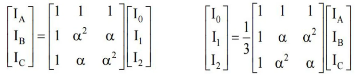
Symmetrical components, denotedI0,I1, and I2, constitute a set of balanced current
phasors representing zero, positive, and negative sequence. This sequence indicates the rotational direction, in the phase plane, in which these phasors cross a reference point,
typically at the0◦ point. Each phase component can be represented as a combination of zero, positive, and negative sequence phasors. Figure 3.1 shows the matrix representation of both phase and symmetrical components (left and right, respectively) of the line current
Figure 3.1: (Left) Phase components and (Right) Symmetrical components of the line currents in phasor form. If a set of components is known, the other can be determined from a matrix transformation.αrepresenting a +120◦phase shift.
In general, positive sequence voltage data is most often considered in analysis of grid
operations mainly because these values reflect the stability of active power flow on the grid. This is especially true when workable, though often approximate, power flow solutions are desired during nominal, balanced, 3-phase operation. This research involves analysis of
3.3 Dataset Characteristics
This research uses synchrophasor datasets provided by the Bonneville Power Administration (BPA). These contain archived, operational data captured from within BPA’s balancing area.
These data conform to IEEE C37.118-2011 (described above in section 3.1) and consists of a single year’s worth of data spanning August 2012 to August 2013 from twenty PMU sites. The data set size is 950 GB. Each file in the set typically holds one to five minutes of
data from each of the twenty separate PMU sites. It includes both positive sequence voltage magnitude (V+) and positive sequence voltage phase angle (φ+).
For this work, analysis is centered around φ+. During nominal operations,φ+ varies
slowly in contrast toV+, which can experience sudden changes. Furthermore,φ+trends
similarly between adjacent PMU sites whereasV+can be at different levels along adjacent PMU sites and is also allowed to deviate±10% from its nominal voltage of 500 kV (1
per unit [p.u.]). Because of these reasons, the methods presented are shown to be highly sensitive to sudden changes inφ+, making it the desirable parameter for use in the analysis.
Justification of this will be reiterated in Chapter 5.3.
Each measurement is given in synchrophasor representation with its associated date/time stamp. The discretization rate between measurements is 16.7 milliseconds (60 phasor measurements/second). The phase angleφ+ is a time-varying real number that oscillates
3.4 Network Topology
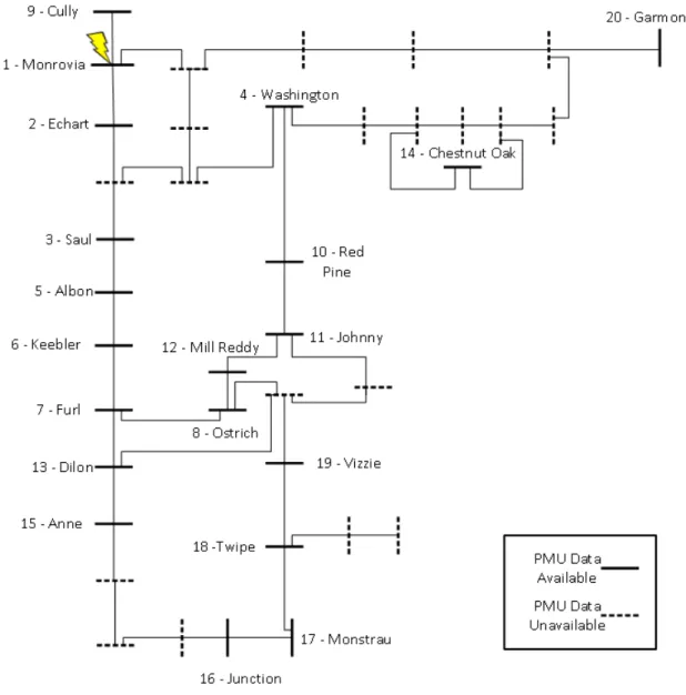
In regards to the synchrophasor network topology, Figure 3.2 provides a general layout of PMU site locations. Although not all PMU sites shown are contained in the dataset (dotted
busses are not included) they are incorporated for the sake of completeness.
Figure 3.2: Synchrophasor network topology represented as a one-line diagram. PMU sites found in the dataset are indicated by solid busses. A lightning strike occurs near PMU site Monrovia and will be presented as a case study. Numbers near site names represent the next closest site to the lightning strike in terms of electrical distance (discussed in further detail in Chapter 4.4).
Our algorithm is tested against power system events that occurred within this system during the August 2012 to August 2013 time period. Instances of lightning strike occurrences have been recorded in the northwest region of Figure 3.2 near PMU site Monrovia. Each
instance led to an occurrence of a line-to-ground fault. Numbers near site names represent the next closest site to the fault in terms of electrical distance (a concept covered in Chapter 4.4). These are the power system events that serve as test cases presented in Chapter 5.
4 Design Methodology
4.1 Correlation
Correlation is a common statistical method used to determine if relationships exist between two continuous variables. The method presented here utilizes a linear statistical method
known as Pearson correlation. To assess the linear relationship between variables, the Pearson correlation coefficient (PCC),r, from recent works [14], is determined based on the following equation: r= cov(X, Y) σXσY = Σ(XY)− ΣXΣY N q (Σ(X2)−(ΣX)2 N )×(Σ(Y2)− (ΣY)2 N ) (4.1)
where cov is the covariance, σX is the standard deviation of X, σY is the standard
deviation of Y, and X and Y are two independent continuous variables of size N.
The output ofris such that−1≤r ≤1wherer=−1represents a perfectly negative linear relationship, r = 1 represents a perfectly positive linear relationship, and r = 0
represents an inconclusive relationship. It has been established that |r| ≥ 0.9 can be interpreted as being ‘very highly’ correlated, 0.7 ≥ |r| < 0.9 as ‘highly’ correlated,
4.2 Window Length
From Equation 4.1, the independent continuous variables, X and Y, represent vectors of data from particularly selected PMU sites. These vectors can be either positive sequence
voltage magnitude,V+, or phase angleφ+. Since X and Y are of size N, altering the size
over a variety of range values can serve as a feature enabling increased robustness and speed in detection of both data and power system events due to the fact that the cardinality of N
represents the ‘window size’ of correlation when determiningr.
Due to the transient nature of power system events, the window size must be selected to be small enough to detect an event in a timely manner and large enough to capture
the dynamics of the event. In Chapter 5 we show that varying the window size increases robustness at detecting different types of data events and in detecting actual power system events that occur within real systems, but at the cost of increased computational intensity.
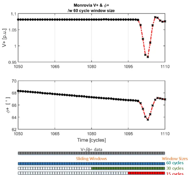
In addition, entries in both X and Y are updated on a cycle-by-cycle basis permitting N to serve as a ‘sliding window’ overV+andφ+data. Figure 4.1 shows bothV+ andφ+data
Figure 4.1: Time domain plot ofV+andφ+ data over a 60 cycle window size during a case study event. Sliding windows with associated window size are depicted at the bottom of the figure. Sliding windows of size N determine the value ofr.
4.3 Correlation Visual
During the early phases of this research, a collaborative effort was made between Oregon State University (OSU), Washington State University Vancouver (WSUV), and Portland
State University (PSU) to develop an event detection algorithm dubbed Correlation Matrix Algorithm (CMA). The CMA facilitates the use of real-time PMU data for detecting and flagging data and event-related issues. Another result of this collaboration was the creation
of an engine that simulates real-time streaming of PMU data. This data stream serves as input into our correlation methods, and provides a visual representation of system-wide correlation, as shown in Figure 4.2.
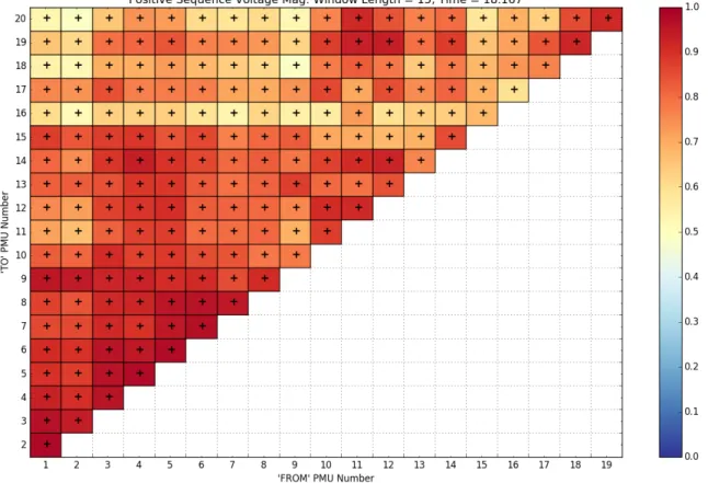
To explain Figure 4.2, let us be explicit of its features. Each coordinate square represents a pairwise correlation value (indicated by the color scale on the right) between ‘FROM’ and ‘TO’ PMU numbers. The structure takes an upper triangular shape due to the pairwise
nature of correlation. The sign of the correlation is indicated in the center of each coordinate square as either a+, or−symbol. When correlation is inconclusive, a∅symbol will be present and the coordinate square will be blacked out. The title, at the top of the figure,
indicates the attribute (V+orφ+), window size, and time of latest entry (in seconds) being
Figure 4.2: Visual representation of system-wide correlation utilizing a 15 cycle window size over nominalV+ data (void of any data/event-related issues) for a system containing 20 PMUs.
4.3.1 Historic Playback Engine
This collaboration resulted in co-development of a real-time, data-playback engine that analyzes characteristics of the dataset. The engine streams archived PMU data as input into the CMA effectively linking raw power system data and our correlation methodology.
By understanding the file traits, recorded power system attributes, data discretization rate, and topological layout of the PMUs (depicted in Figure 3.2), aPhasor Data Concentrator
(PDC)engine was created. Often, PMUs located at different points around the grid are grouped by zones, and consequently their data streams are multiplexed to a single data
logging point. This central data entry point is what is commonly referred to as a PDC. The PDC engine serves a similar purpose by replicating a single multiplexed data stream based on the archived operational PMU data, thus simulating the real-time power system
operation.
4.3.2 Data Structure
As positive sequence voltage data is processed in the time-domain by the PDC engine, the data are written into the working memory of the correlation algorithm. In an effort
to minimize computational complexity, a custom data structure was developed to quickly append new data, reference data already stored, and account for multiple characteristics such as time, magnitude, phase, and correlation coefficients for each of the 20 PMUs. This
As seen in Figure 4.3, the lowest layer of the data management system holds the actual values read in from the PDC feeder as well as the calculated correlation coefficients (referred to as “Correlation Objects"). These Correlation Objects are dynamically created based
on the number of multiplexed PMUs. This reduces redundancy of data in the correlation technique since Correlation Objects represent a combination of two PMUs. The next layer of the management system is made up of Correlation Object combinations at a specific time
stamp (referred to as “Time Structure"). This creates a triangular matrix of Correlation Objects that reference both a unique time as well as the PMU data and correlation value at that particular time. Finally, at the highest management level, each Time Structure is stored
in a queue of dynamic length. The PMU and correlation data can effectively be monitored in the time domain for any desired window size.
4.4 Electrical Distance
The concept of electrical distance is applied when deciding which PMUs to cluster. Electrical distance give a sense for theelectricalproximity between substations, as opposed to physical
distance. As such, two electrically close substations will experience similar responses to a nearby system event, whereas two substations that are electrically-far from each other may not exhibit similar responses to an event. The concept of electrical distance has been
applied to multiple different scenarios, such as multi-objective power network partitioning, identifying structural vulnerabilities, and evaluating marginal loss factors [15–17].
Recall earlier that the Northwest region of Figure 3.2 experienced lightning strike
occurrences near PMU site Monrovia. Figure 4.4 focuses on this region. All available PMUs in this region are labeled in ascending order in terms of electrical distance with respect to site Monrovia and will represent a PMU cluster for a particular case study in Chapter 5.
4.5 Rayleigh Distribution
The distribution to be utilized is a continuous probability distribution known as the Rayleigh distribution, given by recent works [18], is defined as
f(x;σ) = x σ2e −x2 2σ2 |x≥0, σ >0 (4.2)
wherexis the Rayleigh distribution parameter andσis the scale parameter with
σ= v u u t 1 2n n X i=1 x2 i (4.3)
Applications of this distribution can be found in a variety of areas including communications,
image processing, and physical sciences, among others [19–21]. Considering the probability distribution function, selection of this particular distribution was based on the range of values the random variable will be expected to take given it will consist mostly of ’very
highly’ (positive) correlatedrvalues.
However, the range of the Pearson correlation coefficient, r, is such thatr ∈ [−1,1]. Noting that very few of the PMUrvalues are negatively correlated, fewer than 1% forφ+
(10% forV+), we consider just the magnitude ofr, for which|r| ∈ [0,1], or, rather more
namely, its inverse,
y= 1
|r| (4.4)
for whichy∈[1,∞). By definingysuch thaty =x+ 1, the Rayleigh distribution variable can be formally defined as,
x=y−1 = 1
|r| −1 (4.5)
for whichx∈[0,∞).
To follow up on the assumption that solely the magnitude of r can be considered, Table 4.1 shows, for the case study PMU cluster, the amount of negative r entries (in percentage) ofφ+ over a single minute, 1, 2, and 24 hours of nominal data (void of any
data/event-related issues) with 15, 30, and 60 cycle window sizes. It can be observed that there are very few occurrences of negativer values ofφ+, less than 0.33% at worst
(Washington, 30 cycles, 1 minute - seen inbold). Since the amount of negativerentries of
φ+ is disproportionate, these entries can be discarded when analyzing |r| ofφ+.
Considering V+, Table 4.2 shows the amount of negativer entries when applying the
same treatment. It can be observed that up to 6.44% (Washington, 15 cycles, 24 hours - seen
inbold) ofrentries forV+are negatively correlated. Therefore, the assumption that|r|can
solely be considered needs to be revisited for analysis ofV+. This assumption is reiterated
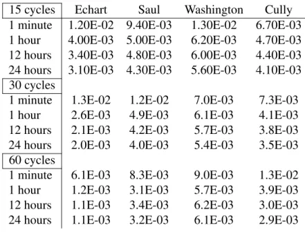
Table 4.1: Negativerentries (in percent) ofφ+for case study PMU cluster over a single minute, 1, 2, and 24 hours of nominal data with 15, 30, and 60 cycle window sizes.
15 cycles Echart Saul Washington Cully 1 minute 0.00 0.08 0.14 0.08 1 hour 0.02 0.16 0.19 0.17 12 hours 0.01 0.15 0.17 0.12 24 hours 0.01 0.16 0.17 0.1 30 cycles 1 minute 0.00 0.00 0.33 0.17 1 hour 0.00 0.08 0.15 0.12 12 hours 0.01 0.10 0.13 0.10 24 hours 0.01 0.10 0.14 0.08 60 cycles 1 minute 0.00 0.00 0.00 0.00 1 hour 0.00 0.04 0.07 0.05 12 hours 0.00 0.03 0.06 0.04 24 hours 0.00 0.04 0.06 0.03
Table 4.2: Negativerentries (in percent) ofV+for case study PMU cluster over a single minute, 1, 2, and 24 hours of nominal data with 15, 30, and 60 cycle window sizes.
15 cycles Echart Saul Washington Cully 1 minute 0.08 1.00 1.03 1.75 1 hour 0.51 4.11 4.47 2.72 12 hours 0.99 5.81 6.03 2.60 24 hours 1.14 5.95 6.44 2.55 30 cycles 1 minute 0.00 0.03 0.72 0.89 1 hour 0.04 2.46 3.31 1.55 12 hours 0.11 3.54 4.10 1.37 24 hours 0.13 3.36 4.05 1.17 60 cycles 1 minute 0.00 0.00 0.06 0.14 1 hour 0.00 1.22 3.16 0.92 12 hours 0.01 2.02 3.43 0.86 24 hours 0.01 1.76 2.93 0.67
Refocusing on characteristics of the Rayleigh distribution, in addition to the Rayleigh
variance, from recent works [18], are defined as, µ(x) =σ r π 2 (4.6) and var(x) = 4−π 2 σ 2 (4.7)
For electrically close PMUs in steady-state, the expected value of |r|is very close to
one, since under steady-state conditions the voltage magnitude and phase angle profiles trend nearly identically. Therefore, deviations from|r| = 1, are very rare. As such, the expected value forxis near zero. This is, in fact, what we observe; observingµ(x)and
var(x)for PMU pairs included in the case study, it can be seen that there is little variation
from steady-state values. Table 4.3 and 4.4 show, for the case study PMU cluster, calculated
µ(x)andvar(x)over a single minute, 1, 2, and 24 hours of nominal data with 15, 30, and
60 cycle window sizes. V+is not given similar treatment and justification for doing so will
Table 4.3:µ(x)ofφ+for case study PMU cluster over 15, 30, and 60 cycle window size.
15 cycles Echart Saul Washington Cully 1 minute 1.20E-02 9.40E-03 1.30E-02 6.70E-03 1 hour 4.00E-03 5.00E-03 6.20E-03 4.70E-03 12 hours 3.40E-03 4.80E-03 6.00E-03 4.40E-03 24 hours 3.10E-03 4.30E-03 5.60E-03 4.10E-03 30 cycles
1 minute 1.3E-02 1.2E-02 7.0E-03 7.3E-03 1 hour 2.6E-03 4.9E-03 6.1E-03 4.1E-03 12 hours 2.1E-03 4.2E-03 5.7E-03 3.8E-03 24 hours 2.0E-03 4.0E-03 5.4E-03 3.5E-03 60 cycles
1 minute 6.1E-03 8.3E-03 9.0E-03 1.3E-02 1 hour 1.2E-03 3.1E-03 5.7E-03 3.9E-03 12 hours 1.1E-03 3.4E-03 6.2E-03 3.0E-03 24 hours 1.1E-03 3.2E-03 6.1E-03 2.9E-03
Table 4.4:var(x)ofφ+for case study PMU cluster over 15, 30, and 60 cycle window size.
15 cycles Echart Saul Washington Cully 1 minute 1.50E-03 2.70E-03 2.30E-03 1.90E-03 1 hour 5.90E-04 1.30E-03 2.30E-03 1.30E-03 12 hours 5.60E-04 1.40E-03 2.10E-03 1.20E-03 24 hours 5.40E-04 1.40E-03 2.10E-03 1.10E-03 30 cycles
1 minute 2.30E-03 4.40E-03 8.00E-03 1.30E-03 1 hour 3.80E-04 1.40E-03 2.20E-03 1.20E-03 12 hours 2.60E-04 1.00E-03 2.30E-03 9.70E-04 24 hours 2.70E-04 1.00E-03 2.20E-03 8.10E-04 60 cycles
1 minute 2.60E-04 9.50E-03 1.60E-03 1.20E-03 1 hour 3.20E-05 6.40E-04 2.10E-03 5.20E-04 12 hours 8.00E-05 5.40E-04 2.60E-03 5.90E-04 24 hours 8.90E-05 5.40E-04 2.60E-03 5.20E-04
It is expected that a disproportionate number ofx=∞(r= 0) values from our PMU
drifts and other very strong data-related decorrelation events. As such, these values are neglected when fitting the Rayleighσto the Rayleigh distribution.
4.5.1 Event Detection Metric
Forx values that conform to the distribution, these are used to derive metrics for power
system event detection. Specifically, monitoringxfor deviations outside a multiple, K, of the variance can be used as a metric for detecting events defined as
x > µ(x) +Kvar(x) (4.8)
where K is an integer multiple. Becausexis a fractional number, typicallyx <1×10⁻³
when in steady-state as shown at the top portion of Table 4.3, Equation 4.8 is normalized by the mean. From Table 4.4,µ(x)is approximately1×10−4. Normalizing Equation 4.8 then
becomes x µ(x) >1 +K var(x) µ(x) (4.9) where values of x
µ(x) will be, by definition, approximately equal to1, and
var(x)
µ(x) will be
approximately 1
10 (from Table 4.3 and 4.4), both during steady-state. When normalized, 1 +Kvar(x)
µ(x) is used as theevent detection threshold valueand Equation 4.9 is theevent
detection threshold inequality.
To establish this detection threshold value, a setup time over nominal data is first
of raw data analyzed. Lastly, to establish steady-state values forσ, a single minute (3600 cycles) in total of raw data is analyzed before establishing the var(x)
µ(x) component.
To show the viability of this detection metric, over a full minute of data containing
an event, the normalized xis plotted and the threshold value imposed for a particular K value and site pair. Prior-event and post-event data is indicated with a dotted blue marker, a dotted red marker indicates the event occurrence (starting at cycle 1100 with a duration of
approximately 10 seconds), and the established threshold value indicated with a solid black horizontal line in Figures 4.5, 4.6, and 4.7. Any normalizedxwhich exceeds the threshold value is differentiated with a red ‘o’ marker. Furthermore, any normalizedxwhich exceeds
the threshold value prior and post event lightning strike will be classified as a false-positive and differentiated with a blue ‘+’ marker.
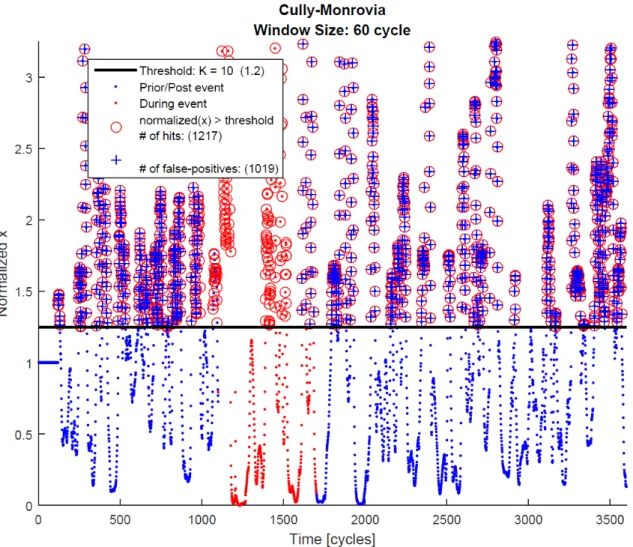
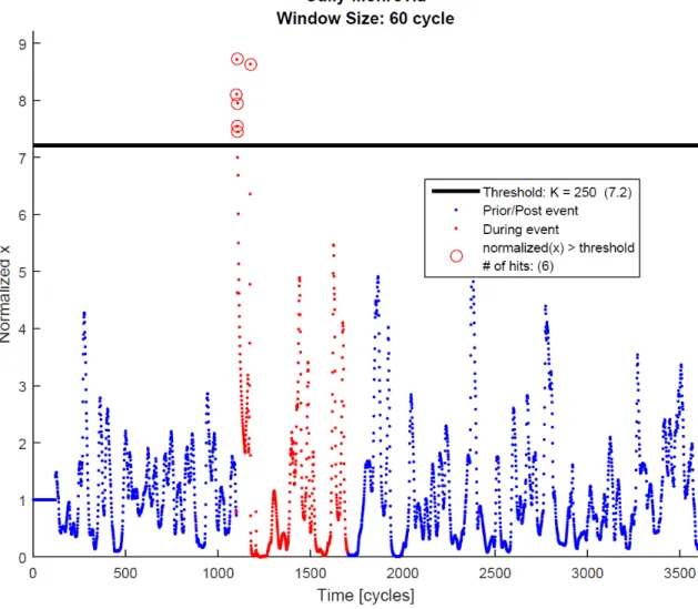
To demonstrate this metric over a 60 cycle window size, PMU site Cully is selected from
the case study cluster and a set of K values chosen for testing purposes. LettingK = 10,100,
and250, from the legend in Figures 4.5, 4.6, and 4.7, the number of normalizedxvalues exceeding the threshold value is 1217, 141, and 6 (respectively) while the false positives are
1019, 106, and 0. WhileK = 250preserves event detection and includes no false-positives, this value does not represent the optimal K as it is higher than necessary, adversely affecting
Figure 4.5: Plot of normalizedxofφ+over a 60 cycle Ksweep size with threshold value such thatK= 10. The amount of data presented represents approximately 60 seconds of raw data prior/post and including lightning strike occurrence as shown in blue and red dot markers, respectively. Normalizedxwhich exceeds the threshold (shown as solid black horizontal line) are indicated by red ‘o’ markers. The first row in the legend shows the K value which establishes the threshold value (shown in parenthetical). The last two row entries in the legend displays the amount of normalizedxexceeding the threshold and the classified false-positives (1217, 1019 respectively).
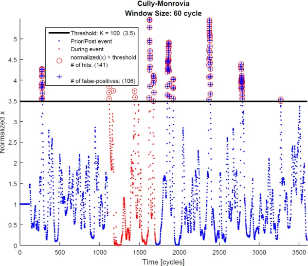
Figure 4.6: Plot of normalizedxofφ+over a 60 cycle window size with threshold value such thatK= 100. With this K value, 141 entries exceed the threshold value with 106 false-positives (some entries not shown), implying that this K is too sensitive, flagging many false-positives.
Figure 4.7: Plot of normalizedxofφ+over a 60 cycle window size with threshold value such thatK= 250. With this K value, six entries exceed the threshold value (some entries not shown) with no false-positives, implying that this K value securely detects this lightning strike occurrence. It is not, however, the optimal K as it is higher than necessary, adversely affecting event detection.
By sweeping through a range of K values, the sensitivity of the threshold value to event
detection and false-positive classification is investigated. Table 4.5 shows this sweep over a range of K values. As expected, a lower K flags for more false-positives than a higher K. Noting this sensitivity, the problem now becomes selecting an optimal K which minimizes
Table 4.5: Sweep of K values to determine amount of normalizedxexceeding threshold and classified false-positives (the latter shown in parentheses).
K (based on 15 cycles)
Echart Saul Washington Cully 1 1804 (1531) 1692 (1411) 1698 (1424) 1715 (1474) 5 1498 (1261) 1325 (1084) 1349 (1119) 1311 (1102) 10 1149 (939) 956 (755) 918 (734) 913 (742) 25 471 (335) 283 (201) 237 (145) 249 (150) 50 119 (63) 39 (21) 29 (13) 39 (14) 100 3 (2) 0 (0) 0 (0) 0 (0) K (based on 30 cycles) 1 1742 (1471) 1560 (1269) 1532 (1276) 1537 (1317) 5 1603 (1340) 1247 (993) 1022 (815) 1038 (859) 10 1451 (1204) 929 (721) 641 (465) 658 (539) 25 1033 (845) 386 (269) 129 (76) 177 (106) 50 590 (451) 80 (47) 10 (3) 25 (8) 100 202 (116) 6 (1) 0 (0) 0 (0) K (based on 60 cycles) 1 1617 (1411) 1445 (1165) 1387 (1167) 1519 (1277) 5 1549 (1348) 1134 (921) 1183 (985) 1380 (1159) 10 1479 (1282) 841 (674) 1007 (833) 1217 (1019) 25 1291 (1104) 274 (199) 609 (487) 837 (678) 50 947 (788) 86 (60) 221 (173) 398 (310) 100 474 (366) 3 (0) 22 (11) 141 (106)
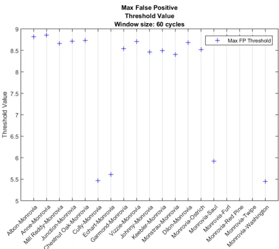
For this particular event, in order to eliminate the event detection threshold inequality (given in Equation 4.9) from evaluating true due to false-positives, the threshold must be set higher than the maximum normalizedxvalue pre-event or post-event. This value, referred
to from here on as themaximum false-positive threshold value (MFPTV), is determined over data void of any data-related events, for all PMUs paired with Monrovia over a 60 cycle window size. Figure 4.8 indicates these values with a blue ‘+’ marker. For each PMU pair,
taking the ceiling of the MFPTV signifies the lowest allowable value the threshold should be set to in order avoid erroneously flagging normalizedxvalues as indicative of a power system event occurrence.
Figure 4.8: Maximum false-positive threshold value (MFPTV) for all PMUs paired with Monrovia during a minute of data containing the lightning strike occurrence. For a particular PMU, in order to avoid having the event detection threshold inequality evaluate true during normalizedxvalues not associated with the event, the threshold should be set slightly higher than the value indicated with a blue ‘+’ marker. These values were determined over data void of any data-related issues, and, when analyzing normalizedxover a 60 cycle window size.
In a similar fashion, in order to preserve event detection, the event detection threshold inequality must evaluate true at least once during the event. This value, referred to from here
Figure 4.9: Maximum true-negative threshold value (MTNTV - shown with red ‘o’ markers) imposed on maximum false-positive threshold value (MFPTV - shown with blue ‘+’ markers) for all PMUs during a minute of data containing an event. For a particular PMU, in order to preserve event detection, the threshold should not exceed this value.
red ‘o’ marker and imposes them on Figure 4.8. For each PMU pair, the MTNTV signifies
the largest value the threshold can be set to in order to detect normalizedxvalues during the event occurrence.
4.6 Data Events
Given that higher-level applications may become reliant on PMU-generated data, it is of absolute importance to ensure and maintain integrity of incoming data. In this respect,
computation ofrcan be impacted by occurrences of two known types of data events. These include data ‘drop outs’ in which data streams will produce a ‘0’ value when deemed unreliable, and ‘stuck at’ data issues in which case a PMU produces a repeated value. The
latter occurs when a PMU losses synchronicity with the GPS system. These data issues have been dubbed as data drops and data drifts (respectively). These issues must be contended with in order to avoid insecure operations from occurring due to misinformation being
operated on erroneously. A metric to handle these known issues has been devised and is discussed in Chapter 5.1.
To explain how correlation is impacted when data issues are encountered, the visual
structure can be observed. Figure 4.10 provides a correlation visual forφ+when data issues
are being read into the PDC engine. Characteristics of data drop issues include entire rows and columns showing inconclusive correlation (r= 0). Similarly, data drift issues can be
characterized by blacked out rows and columns with a null symbol. This occurs when the standard deviation of either one or another PMU,σX orσY, goes to zero due to repeated
values being reported. With σX and σY in the denominator of the Pearson correlation
Figure 4.10: Visual structure of correlation coefficients during a data drop (upper) and data drift (lower). Correlation coefficients portray signature characteristics of data event occurrences. Characteristic of data drops, entire rows and columns of inconclusive correlation (r= 0) as shown in the upper figure due to a data drop at PMU Number 5. Characteristic of data drifts, entire blacked out rows and columns shown in the lower
4.7 Power System Events
In regards to power system events,rhas been observed to become decorrelated regressing from a ‘very highly’ correlated state to a lower state of correlation. The severity of
decorrela-tion depends on two factors; electrical proximity and window size. For instance, electrically close sites regress to ‘moderately’ correlated within a time frame approximately equal to
1
3 of the window size when using 15 and 30 cycle window sizes and approximately 1 2 of
the window size when using a 60 cycle window size. Comparing with electrically-far sites, correlation regression ofr to ‘moderately’ correlated happens in approximately 12 of the window size when using 30 and 60 cycle window sizes but will never leave a ‘very highly’
state when using a window size of 15 cycles.
To explain how correlation is impacted during an event, the visual structure can again be used. Figure 4.11 provides a correlation visual of φ+ over a 30 cycle window size,
qualitatively highlighting an event occurrence. Characteristics of this include varying levels of poorly correlated rows and columns. Most notable here is PMU Number 1, representing PMU site Monrovia, slowly becoming decorrelated with the rest of the system,
thereby indicating a sudden change in φ+. In addition, PMU Number 2, representing
PMU site Echart, exhibits similar behavior but to a lesser extent. This indicates that the event happened between these two sites. It can be seen that the organization of PMUs will
Figure 4.11: Visual structure during an event. Correlation with the sites experiencing an event most strongly (in this instance PMU Number 1 - Monrovia and PMU Number 2 - Echart) have become decoupled, indicating an event has occurred between these sites. Characteristics of an event are rows and columns exhibiting varying levels of poor correlation. When sites are arranged by electrical distance (w.r.t. the event), a gradient of correlation (rdecreases as electrical distance increases) emerges within the visual structure.
4.8 Cluster Size
To choose which PMUs are ideal for monitoring, the MFPTV and MTNTV are used to eliminate unnecessary PMUs and select those that are least likely to flag false-positives. It
can be observed from Figure 4.9 that there exist some MFPTV > MTNTV. This implies that this PMU pair will always report an event due to a false-positive. As such, these PMU pairs should be excluded from being clustered. Figure 4.12 excludes these PMUs in order to
observe which remaining PMU pairs may suitable for clustering.
clustered. Some PMU pairs exhibit small MFPTV. These are most suitable for monitoring as they decrease the probability of flagging for false-positives and better preserve event detection. Figure 4.13 focuses on these PMUs. Since large window sizes will be used to
detect events and small window sizes to confirm they are not data-related, this approach to determining which PMUs to cluster is only performed for a large window size. It should be noted that these PMUs represent the case-study cluster and, due to the reasons above, justify
their inclusion into the cluster.
Figure 4.13: PMUs with MTNTV > MFPTV and with lowest MFPTV are shown. These PMUs represent those found in the case-study cluster.
4.9 Cluster Content
As a recap, a cluster is comprised of a subset of PMU sites containing a combination of electrically near and far sites with respect to the site experiencing the event. Clusters
containing only ‘near’ PMU sites, such as the one shown in Figure 4.14, may not be sufficient for properly detecting the event asrwill remain highly correlated given the similar responses that adjacent sites will exhibit. Additionally, clusters possessing all far PMU sites, such as
the one shown in Figure 4.15, will led to inadequate event detection as correlation will vary having some strongly and weakly correlatedr.
To address this, clusters are comprised of a combination of both near and far sites. This
clustering scheme will be investigated and justified in Chapter 5. This will be shown to be most successful at detecting events; far PMU sites begin to decouple easily due to large electrical distance allowing for detection of event occurrences while near PMU sites can
confirm that the event has occurred based on its nearrvalue since they experience nearly the same degree of impact.
5 Results & Analysis
To facilitate in development of an event detection algorithm, BPA has provided an event log summarizing locations, times, and causes of all known events that occurred during this time frame. The amount of events capturing during this time totals a count of five. Of these five
events, three of them were lightning strike occurrences at or near site Monrovia. The other two events, one due to foreign trouble and the other a lightning strike occurrence, occurs at PMUs which were not included in the dataset. Due to the limited availability of event data,
this section focuses on the three lightning strike occurrences near PMU site Monrovia. Analysis in this section is centered around the particular case study cluster discussed in Chapter 4.8 and depicted in Figure 4.4. TheV+andφ+time domain profiles of this PMU
cluster are shown in Figure 5.1 over a 15 cycle window size with the event differentiated from nominal data (shown by green-dotted, o-marked portions) by red-dotted, x-marked portions. The cluster has been arranged by ascending order of electrical distance (relative
to the event). This window size is selected to best depict the subtle transient nature of the disturbance.
5.1 Detecting Data Errors and Power System Events
As mentioned previously, integrity of PMU data must be preserved in order to ensure reliable operations are performed.
Modifying the Monrovia data stream to contain a 3-cycle data drop (shown at top of Figure 5.2) , the adverse impact at the correlation layer produced by such an occurrence is depicted on the bottom of Figure 5.2 and demonstrates the capability of detecting this type
of data error.
Additionally, when PMUs consecutively produce a constant value (i.e. a data drift), correlation is also adversely affected. To exemplify this type of data event, 20 cycles
of data were duplicated within the Monrovia data steam. Figure 5.3 demonstrates the impact on correlation when observed with 15, 30, and 60 cycle window sizes (from top to bottom, respectively). When observingrover a 15 cycle window size, Monrovia quickly
becomes decorrelated from the rest of the system transitioning from ‘very highly’ to ‘low’ correlation over nearly a single window size. After an entire window size, correlation becomes undefined (shown by the absence of r1035). Correlation remains ‘very highly’
correlated for the larger window sizes. However, correlation barely deviates from r = 1
when approximately 1
4 of the entries are constant for a 60 cycle window size.
Recall the denominator term of Equation 4.1 will be zero when either X or Y does
not vary over the window size, N, resulting inr to be undefined. This is the case when observing the absence of the last entry in the correlation layer under a 15 cycle window size. Therefore, smaller window sizes are excellent candidates for detecting these types of
data issues; flagging data streams which exhibit this behavior as a false-positive and not as an indication of an actual event. The visual structure quantitatively depicts these types of occurrences in Chapter 4.10.
In regards to power system events, the case study indicated in Figure 4.4 of Chapter 4.4 will be analyzed. Figure 4.1 depicts the lightning event in the time domain for the Monrovia site and Figure 5.1 portrays the response of the overall cluster.
5.2 Window Length
In Section 5.1, varying the window size affected the sensitivity of the algorithm in detecting a data drift event. In this case, a smaller window size may be used to detect these type of
data integrity issues, classifying it as a false-positive.
To increase robustness in event detection, varying the window size is a technique for observing the impact onµ(x)andvar(x)of the case study cluster. Figures 5.4 and 5.5
show how these parameters vary 13 cycles into the event (start of the event indicated by red vertical line). It is observed that as window size increases, bothµ(x)andvar(x)decrease.
To quantitatively see this robustness, the correlation visual is used. Figure 5.6 shows
howr varies, with window size, 13 cycles into the event. Over larger window sizes the correlation visual is highly correlated during steady-state, represented as all red coordinate squares. During an event, larger window sizes show correlation slowly regressing, as shown
in the bottom of Figure 5.6, which indicates an event occurrence. Visuals with smaller window sizes are then used to confirm that this regression in correlation is not due to a data issue but is, in fact, an actual power flow contingency. This demonstrates that using multiple
To take full advantage of this robustness, multiple detection algorithms with each using different window sizes should be used to monitor a data stream concurrently. In this fashion, when data events occur they can be detected sooner with smaller window sizes, informing
larger window sizes of the data issue. Similarly, when power system events occur they can be detected as such by larger window sizes and confirmed with smaller window sizes. This advantage is only made possible when a minimum of two detection algorithms are used;
5.3 Rayleigh Characteristics
Given the presumed fluctuating nature intrinsic toV+, it is expected thatvar(x)exhibits
more volatility compared toφ+. The difference in scale is stark, V+ being1×105 times
more, as can be observed along the y-axis ofvar(x)plots shown in Figure 5.7. As such, analyzingφ+proves more useful for event detection due to the variance exhibiting sensitivity
to sudden drastic changes withφ+.
Additionally, Table 4.2 in Chapter 4.5 showed up to 6.44% ofrvalues are negative for
V+. Given the above statements about volatility and considerably higher occurrences of
negativerentries, analysis ofµ(x)andvar(x)were not performed forV+.
When observing the Rayleigh distributions ofφ+ over nominal data, the distributions
(shown in top portion of Figures 5.8, 5.9, and 5.10 for 15, 30, and 60 cycle window sizes, respectively) resemble the expected profile of a general Rayleigh probability density function
(PDF). However, when observing 13 cycles into the occurrence of a lightning strike event,
xdeviates from its previous distribution profile quite drastically, as shown in each bottom portion of the respective figure (distinguished with red ’x’ marker). This rapid occurrence
of large outliers is what we use to detect power system events. As a note, both axes on the distribution are held constant for comparative purposes.
To re-enforce understanding of this event detection metric, lets us observe how instances
Figure 5.7:var(x)ofV+andφ+over 30 cycle window size during steady-state just prior to an event. The difference invar(x)is several orders of magnitude as shown by the different scales of the y-axes.
At the instant the lightning strike occurs, a line-to-ground fault takes place near Monrovia, causing a sudden change in real power flow1indicated by the time domain profile of φ
+,
depicted previously in Figure 4.1 of Chapter 4.2. Recall from Chapter 3.3 the primary reason
φ+ is selected as the parameter to analyze is because it varies slowly (in contrast toV+)
and it trends similarly between adjacent PMU sites causingr(φ+) to be highly sensitive to
impulse events that alter real power flow. Observing Equation 4.5,
x=y−1 = 1
|r| −1
noting thatr(φ+) determines its value,xshould remain approximately zero during
steady-state. With the sensitive nature ofr(φ+) in mind, a lightning strike event causes an abrupt
change in real power flow, and more directlyr(φ+), which is in fact what is captured and
signified byxoutliers in the Rayleigh distribution as shown at the bottom of Figures 5.8, 5.9, and 5.10.
During an event, as shown from the bottom of Figures 5.8, 5.9, and 5.10, as window size increases the x-axis decreases. Comparing Figure 5.9 to Figure 5.8, a decrease in scale, as much as 49%, can be seen along the x-axis. Comparing Figure 5.10 to Figure 5.9, a
decrease in scale, as much as 38%, can be seen along the x-axis. This implies that, with larger window sizes, the sensitivity of the algorithm decreases when analyzingφ+sincex
will exhibit small variations, compared to smaller window sizes, which will exhibit much
Figure 5.8: Rayleigh distribution ofφ+over 15 cycle window size with x-axis held constant for comparative purposes. (Top) Steady-state profile of Rayleigh prior to lightning strike. (Bottom) 13 cycles into a lightning event causingxto deviate from steady-state. Note the change of scale of the x-axis from steady-state data to
Figure 5.10: Rayleigh distribution ofφ+over 60 cycle window size with x-axis held constant for comparative purposes. (Top) Steady-state profile of Rayleigh prior to lightning strike. (Bottom) 13 cycles cycle into a lightning event causingxto deviate from steady-state. Further, note the decrease of the x-axis scale from the
To quantify the change in the spread ofxfrom steady-state to the event, when observing each PMU pair for each individual window size,σ can be fitted to the Rayleigh distribution during these two instances. First,σis determined during steady-state (denotedσss) and 13
cycles into the event (σevent). Next, the
σevent
σss
ratio is determined for all clustered PMU pairs over 15, 30, and 60 cycle window size scenarios. Table 5.1 shows the σevent
σss
ratio for all clustered PMU pairs over 15, 30, and 60 cycle window size scenarios.
Table 5.1: Quantifying the change in the spread ofxof the Rayleigh distribution, during the lightning strike event compared to steady-state. Taking the ratio ofσ13 cycles into an event overσduring steady state quantifies the change in the spread ofx. Based on PMU pair, this ratio trends differently while increasing window size; Echart increases, whereas the rest vary. These, however, possess a smaller σevent
σss
ratio when going from a 15 cycle window size to a 60 cycle window size.
15 cycles Echart Saul Washington Cully 2.20E+02 5.20E+02 3.80E+03 2.00E+03 30 cycles
7.80E+02 6.10E+02 4.20E+03 2.90E+03 60 cycles
1.40E+03 3.80E+02 1.10E+03 1.30E+03
From Table 5.1, based on the observed PMU pair, σevent
σss
trends differently when increas-ing window size. For instance, based on Echart, σevent
σss
will increase with larger window
sizes, whereas Saul, Washington, and Cully will vary. These sites, however, will remain consistent in that they possess a smaller σevent
σss
ratio when going from a 15 cycle window size to a 60 cycle window size.
5.4 Cluster Scheme
To achieve maximum system monitoring, one might hypothesize that all PMU combinations within a balancing area must be correlated. This is, however,notnecessary. To optimize
event detection capabilities while preventing unnecessary and/or redundant computation, the algorithm need only monitor a subset of PMUs, so long as that cluster contains including both electrically-near and far PMUs. A near-far cluster of PMUs offers advantages over
all-near or all-far clustering schemes. Recall from Chapter 4.9, using an all-near clustering scheme provides no reference to what constitutes an event; similarly for an all-far clustering scheme. By clustering a combination of both near and far PMUs and observing at the
correlation layer, an event occurrence can be detected via far sites since correlation becomes decoupled with electrical distance. Furthermore, the event can be confirmed via near sites since adjacent sites experience events in a similar fashion and so theirφ+will trend similarly.
In order show viability of this clustering scheme, the case study cluster will be concur-rently analyzed with one small and one large window size. Figure 5.11 plots the normalized Rayleigh distribution variable,x/µ(x), prior to a lightning strike event, as shown with blue
‘.’ markers. Each PMU pair has its own predetermined threshold value, shown within the title portion of the PMU pair in parenthesis. Recall from Chapter 4.5.1, these threshold values were established to be the lowest allowable value which does not classify false-positives
Observing 13 cycles into the event, Figure 5.12 imposes these threshold values as a solid black horizontal bar and shows event-related data that does not exceed the threshold value as red ‘.’ markers. Normalizedxvalues that exceed the threshold are shown as red ‘x’ markers.
From Figure 5.12, observing the 15 cycle window size scenario, normalizedxvalues will begin to exceed the threshold value a few cycles into the event. About five cycles in, however, a majority of the normalized xvalues go below the threshold value. Some
sites, namely Cully, will experience normalizedxvalues oscillate about the threshold value repeatedly. Declaring an event basedsolelyon this window size would be inadequate given the limited amount of time to declare the event and the uncertainty caused by the oscillation
at Cully.
Now, observing the 60 cycle window size, normalized xvalues exceed the threshold within a few cycles into the event as well. Moreover, nearly all normalizedxvalues continue
to exceed the threshold value 13 cycles into the event for all PMUs. To ensure no oscillations occur, as with Cully in the 15 cycle window size scenario, Figure 5.13 observes the 60 cycle window size scenario 40 cycles into the event. It can be seen that normalizedxvalues
gradually decrease towards its steady-state profile. Therefore, a large window size can be used with certainty to detect the event occurrence while a small window size can confirm
that an actual power system event. This demonstrates that concurrent analysis with two window sizes over this clustering scheme is viable for detecting these types of events in this area of the synchrophasor network.
Figure 5.13: Normalizedxvalues, 40 cycles into the lightning strike occurrence, for the case study cluster over a 60 cycle window size. This is done to ensure no oscillations of normalizedxoccur about the threshold as shown in Figure 5.12 with the 15 cycle window size.
5.4.1 Analyzing Other Events
In order to verify this clustering scheme provides adequate detection, the remaining events were analyzed in a similar fashion to the above. Unfortunately, all of these events occur at or near the same location. Regardless of this limitation, Figure 5.14 shows the time domain
response for site Monrovia and Cully during another lightning strike event, dubbed event 2. Figure 5.15 shows the time domain response over the case study cluster. Figure 5.16 depicts the visual structure 13 cycles into the event over the entire system. Figures 5.17 and 5.18
show the normalizedxprior to and 13 cycles into the event, over a 15 and 60 cycle window size. Analysis occurs over the same case study cluster but differs from the previous event in that the established threshold values are unique to this event.
Figure 5.14: Time domain response ofV+andφ+, for Monrovia and Cully, 40 cycles into event 2 over a 60 cycle window size.