Reinforcement Learning for Automatic Online Algorithm Selection - an
Empirical Study
Hans Degroote1, Bernd Bischl2, Lars Kotthoff3, and Patrick De Causmaecker4 1 KU Leuven, Department of Computer Science, CODeS & iMinds-ITEC, Belgium
2 Bernd Bischl, Department of Statistics, LMU Munich 3 University of British Columbia, Department of Computer Science 4 KU Leuven, Department of Computer Science, CODeS & iMinds-ITEC, Belgium
Abstract: In this paper a reinforcement learning methodol-ogy for automatic online algorithm selection is introduced and empirically tested. It is applicable to automatic algo-rithm selection methods that predict the performance of each available algorithm and then pick the best one. The experiments confirm the usefulness of the methodology: using online data results in better performance.
As in many online learning settings an exploration vs. exploitation trade-off, synonymously learning vs. earning trade-off, is incurred. Empirically investigating the qual-ity of classic solution strategies for handling this trade-off in the automatic online algorithm selection setting is the secondary goal of this paper.
The automatic online algorithm selection problem can be modelled as a contextual multi-armed bandit problem. Two classic strategies for solving this problem are tested in the context of automatic online algorithm selection: ε-greedy and lower confidence bound. The experiments show that a simple purely exploitative greedy strategy out-performs strategies explicitly performing exploration.
1
Introduction
The problem considered in this paper is automatic algo-rithm selection. The field of algoalgo-rithm selection is mo-tivated by the observation that a unique best algorithm rarely exists for many problems. Which algorithm is best depends on the specific problem instance being solved. This can be illustrated by looking at the results of past SAT-competitions1. There are always problem instances that are not solved by the winning algorithm (the overall best) but that other algorithms manage to solve [25].
The complementarities between different algorithms can be leveraged through algorithm portfolios [13]. In-stead of using a single algorithm to solve a set of prob-lems, several algorithms are combined in a portfolio and a method of selecting the most appropriate algorithm for each problem instance at hand is used. This selection pro-cess is called automatic algorithm selection.
State of the art approaches for automatic offline algo-rithm selection use machine learning techniques to create a predictive model based on large amounts of training data.
1http://satcompetition.org/
The predictive model predicts for each instance which al-gorithm is likely to be best. The model is created based on characteristics of the problem under consideration. These characteristics are called problem features. The idea is that their value should be correlated with how hard a problem is for a certain algorithm.
Automatic algorithm selection methods are metaheuris-tics in the sense that they are general problem-independent strategies with a different implementation depending on the specific problem being considered. The difference in implementation manifests itself in the choice of features, which are distinct for every problem. For example, the ra-tio of the amount of clauses over the amount of variables is relevant for satisfiability problems but makes no sense for graph colouring or scheduling problems.
After the training phase the decision model remains fixed in automatic offline algorithm selection. To decide which algorithm to use to solve a new instance with, its features are calculated and input into the decision model which in turn returns an algorithm. This algorithm is then used to solve the instance with.
The observation motivating this research is that new performance data keeps being generated after the training phase every time the predictive model is used to predict the best algorithm for a new instance. This data is freely available yet not used by automatic offline algorithm selec-tion methods. The main research quesselec-tion of this paper is: “Can online performance data be used to improve the pre-dictive model underlying automatic algorithm selection?". An interesting challenge faced in automatic online al-gorithm selection is finding a balance between learning a good predictive model and making good predictions. Se-lecting a predicted non-best algorithm might be better in the long run because the information thus obtained results in a better model and more accurate predictions for fu-ture instances, but it negatively affects the expected per-formance on the current instance. This challenge is an example of the exploration vs. exploitation trade-off of-ten faced in reinforcement learning. It is also called the learning vs. earning trade-off.
The automatic online algorithm selection problem can be modelled as a multi-armed bandit problem, more specifically as a multi-armed bandit problem with covari-ates, also known as the contextual multi-armed bandit
problem, as for each problem instance the values of a num-ber of problem characteristics are known. Two basic clas-sic strategies for solving the contextual multi-armed ban-dit problem that incorporate explicit exploration are tested and compared to the purely exploitative approach.
The remainder of this paper is structured as follows. In section 2 the automatic online algorithm selection problem is defined. First the classic automatic offline algorithm se-lection problem is discussed, then the methodology for au-tomatic online algorithm selection is presented after which the contextual multi-armed bandit problem is introduced and is shown how automatic online algorithm selection can be modelled as a contextual multi-armed bandit prob-lem. In section 3 related work is discussed. The exper-imental setting and results are presented in section 4. In section 5 some remarks about the introduced methodol-ogy are made and the experimental results are discussed. Future work is also discussed in section 5. The paper con-cludes in section 6
2
Automatic Online Algorithm Selection
2.1 Automatic Algorithm SelectionRice’s paper "The algorithm selection problem" [23] for-mally introduced the algorithm selection problem. The fundamental characteristics of the problem remain un-changed up to now. In the most basic scenario identified by Rice the problem is characterised by a set of instances, a set of algorithms and a (set of) performance measure(s) and by two mappings between these sets: a selection map-ping and a performance mapmap-ping. The selection mapmap-ping maps instances to algorithms and the performance map-ping maps algorithm-instance pairs to their performance-measure(s). A typical formulation of the objective of auto-matic algorithm selection is to find the selection mapping that results in the best average performance.
It is up to the user to identify a sensible performance measure. In this paper only single-objective problems are considered. See [9] for a more formal description of what characterises an acceptable performance measure for the research in this paper. Each performance measure with totally ordered values is definitely acceptable.
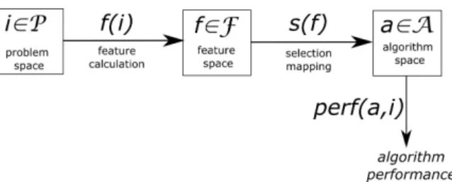
Rice acknowledges the need for a set of features in prac-tical applications and extends his model with this set. The full model is visualised in figure 1. Note that the selection mapping now maps values from the feature space instead of directly from the instance space.
To formalise the problem statement, let Q be a prob-ability distribution on the instance set I. Let f be the feature mapping (mapping an instance to a feature vec-tor),sthe selection mapping (mapping a feature vector to an algorithm) and p the performance mapping (mapping an instance-algorithm combination to a performance mea-sure). The average performance of a selection mapping can now be defined as:
EQ[(p(s(f(i)),i)] (1)
Figure 1: Rice’s model for algorithm selection’
The aim is to find the feature mapping and selection mapping that optimise the average performance. The fea-tures of an instance are given, so the only leeway there is which features to consider. Limitations on the possible se-lection mappings can be imposed by the method used to create it.
Identifying descriptive features is a time consuming process. Luckily large amounts of features have already been proposed in literature for many interesting problems. For example in [22] an overview is given of features for the satisfiability problem and in [21] for the multi-mode resource-constrained project scheduling problem.
The automatic in automatic algorithm selection refers to the way decision models are made: automatically. Super-vised learning techniques are typically used.
Two broad classes of techniques can be identified. In the first fall classification-based techniques: the decision model directly predicts which algorithm will be best for an instance based on its features. No information about the actual quality of the algorithm is communicated. Note that in general this is not a binary but a multi-class clas-sification problem, as each instance is classified as being best-solved by one of an arbitrary amount of algorithms. In [20] for example, the k-nearest-neighbours method is used. Another example of the use of k-nearest-neighbours can be found in [6], where the more complicated problem of ranking algorithms (as opposed to only predicting the best) is considered. Another option is to use decision trees or their more powerful relative random forest, as in the latest version of Satzilla [26], an algorithm selector for the satisfiability problem.
Misclassification is cost-sensitive in automatic algo-rithm selection: classifying an instance incorrectly as be-ing best solved by a horrendous algorithms is worse than classifying it as being best solved by an algorithm only marginally worse than the best one. A classification-based automatic algorithm selection technique should take this cost-sensitivity into account, as argued in [5].
The second class of automatic algorithm selection tech-niques consists of regression-based techtech-niques. A regres-sion model is created for each algorithm, predicting its performance in function of the problem features. The al-gorithm with the best predicted performance is selected to solve a new instance with. An overview of such tech-niques can be found in [14]. A recent approach is de-scribed in [10].
Note that algorithm selection itself is a cost-sensitive classification problem: the goal is to classify instances as belonging to the algorithm that best solves them. The distinction between classification and regression methods refers to how this classification problem is solved behind the scenes.
A thorough overview of algorithm selection methodol-ogy can be found in [24] and more recently in [17].
Both classes of automatic algorithm selection methods use the same kind of input to initialise their decision mod-els: performance data of all algorithms on a set of train-ing instances. For the classification-based techniques it is strictly necessary for the performance of all algorithms to be available for each instance. Otherwise it is not possi-ble to say which algorithm is best for the instance. This is not the case for regression-based techniques. As long as each algorithm’s model has access to datapoints it can be initialised, it is not necessary to know the performance of each algorithm on each training instance.
2.2 Solution Strategy for Automatic Online Algorithm Selection
During the online phase performance data is generated every time a new instance is solved. This performance data consists of the performance of the selected algorithm on the new instance. The performance data of the other algorithms on the new instance is not available. Since this type of data can only be processed by the regression-based methods, the proposed methodology will be limited to regression-based techniques.
The methodology for automatic online algorithm selec-tion is the following. During the offline training phase an initial regression model is trained for each algorithm , us-ing trainus-ing data consistus-ing of algorithm performance on instances described by feature values. During the online phase the algorithm to solve the first online instance with is selected based on the models created during the training phase. The model of the selected algorithm is retrained with the new datapoint. The performance of all other al-gorithms on the instance remains unknown. The algorithm to solve the second online instance with is selected based on the models created after having solved the first instance, thus one of the models has been updated to incorporate the performance information about the first online instance. Selection for the third online instance is influenced by the two previous etc. As more instances are solved, more dat-apoints are gathered and the models are expected to im-prove, which in turn is expected to result in better algo-rithm selection.
2.3 Automatic Online Algorithm Selection Problem Statement
As discussed in section 2.1, the goal of automatic algo-rithm selection is to find the feature mapping and selection
mapping that optimise the average performance as defined in equation 1.
In the setting of this paper the instance set is defined by a fixed set of benchmark instances and the distribution is uniform. The feature mapping is defined by consid-ering all features available for the benchmark instances. The problem of selecting the most informative features is not considered: the feature mapping is fixed. A selection mapping is defined by considering a regression model for each algorithm and selecting an algorithm in function of these predicted values. The most straightforward selection mapping is to select the algorithm with the predicted best performance. This and other options are discussed in sec-tion 2.4. The performance mapping used is discussed in section 4.1.
In the offline setting the selection mapping remains fixed. However, in the online setting it changes over time as more instances are solved. The selection at each point in time depends explicitly on earlier selections. For this rea-son equation 1 cannot be used directly to formally define a general problem statement for automatic online algorithm selection.
In the empirical setting of this paper the quality of a so-lution to the automatic online algorithm selection problem is measured as its average performance on a time-ordered set of instances, as presented during the online phase. The empirical performance measurement process is explained in more detail in section 4 where the experimental setting and results are described.
2.4 Contextual Multi-armed Bandits
In the standard multi-armed bandit a gambler has access to a set of slot machines (bandits) and must decide on a strategy in which order to pull their arms. His goal is to realise as much profit as possible. Each time an arm is pulled the gambler receives a random reward sampled from a distribution belonging to the selected arm. Initially all distributions are unknown, but as the gambler gambles on he obtains more information about the distributions of the available arms and can make more informed choices.
The central dilemma faced by the gambler is whether to keep pulling the arm proven to be best so far or to try another arm about which little is known and that might be better. If the other arm turns out to be more profitable never having explored its potential further would have lost the gambler a lot of money.
See [1] for a formal definition of the multi-armed ban-dit problem. In this paper a number of policies for pulling arms are analysed in terms of how fast the total profit di-verges from the maximal profit in function of the total amount of pulls.
The contextual multi-armed bandit problem generalises the multi-armed bandit problem. To stay within the metaphor: before pulling an arm the gambler sees a con-text vector. This concon-text vector contains values for pre-defined properties that describe the current situation. In
the contextual multi-armed bandit problem the reward of each arm depends on the context. As in the classic multi-armed bandit problem the gambler’s goal is to maximize his profit, but in order to do so he has to learn how the context vector relates to the rewards.
The automatic online algorithm selection problem is a contextual multi-armed bandit problem. Each algorithm is an arm and pulling an arm is the equivalent of selecting an algorithm. When selecting an algorithm for an instance its feature values are known, which is the equivalent of having shown a context vector. Maximizing profit in this context boils down to minimizing the performance differ-ence between the selected algorithm and the actual best algorithm.
A number of solution strategies for the contextual ban-dit have been introduced and analysed in literature, such as LinUCB [7] where the reward is assumed to linearly depend on the feature vector. However, for the prelimi-nary research presented in this paper three straightforward and simple strategies have been implemented.
The first strategy that is considered is the greedy strat-egy. The greedy strategy does not perform any explicit ex-ploration: it always selects the algorithm that is predicted to be best.
The second strategy that is considered is theε-greedy strategy, which is parametrised by a value ε between 0 and 1. The strategy is equivalent with the simple greedy strategy with probability (1−ε) and selects a random al-gorithm with probabilityε.
The third strategy is the is the UCB strategy, short for upper confidence bound. It is parametrised by parameterλ (withλ≥0). The UCB strategy consists of calculating for each algorithm its predicted performance pand the stan-dard error on this predictione. The algorithm with highest value forp+e∗λ is selected. Since algorithms for which few datapoints exist typically have high variance on their predictions, an algorithm with predicted poor performance might be preferred over an algorithm with decent perfor-mance, depending on the performance difference, variance sizes and the value ofλ. A higherλ-value results in more exploration.
The equivalent of the UCB strategy for minimisation problems is the LCB strategy, short for lower confidence bound. Its selection rule is: p−e∗λ.
Unlike the two previous strategies, which only rely on a predicted value, the LCB strategy also relies on a notion of variance. Hence it can be applied only to regression meth-ods for which the variance on a prediction is calculable.
3
Related work
Reinforcement learning and multi-armed bandit method-ology have been applied to some related topics in auto-matic algorithm selection literature. However, the authors believe the setting considered in this paper, applying re-inforcement learning to the standard automatic algorithm
selection problem where one has to select one algorithm from a limited pre-defined set of algorithms to solve an in-stance with, has not yet been investigated. In the remain-der of this section some related research is discussed and is mentioned how it differs from this work.
In [11] multi-armed bandit methodology is applied to the online learning of dynamic algorithm portfolios. Their goal differs from this paper’s. They want to learn for each instance a separate algorithm portfolio while the goal here is to predict one algorithm to solve the instance with. In an algorithm portfolio a bunch of algorithms are run si-multaneously. The dynamic goal is to learn the optimal assignment of time slices to algorithms while the portfolio is in use. This paper’s setting is not dynamic in this sense. Once an algorithm has been selected to solve an instance with this decision will not be come back on, even if the algorithm appears to perform poorly on the instance.
In [8] a new multi-armed bandit model is proposed and applied to search heuristic selection, a kind of algorithm selection. However, their objective differs from this pa-per’s. In terms of algorithm selection they have access to a number of stochastic algorithms and a budget ofNtrials. The goal is to find an as good as possible solution for one instance within the budget ofNtrials, whereas this paper’s goal is to find an as good as possible solution on average over many instances, each with a budget of one trial. Their stochasticity is caused by the algorithms but the instance remains fixed. In this paper stochasticity is also caused by the instances as at each point in time a new random instance is solved.
In [12] a notion of online algorithm selection is intro-duced for decision problems. They focus on the problem of deciding how to distribute time shares over the set of available algorithms and make this decision on an instance per instance basis. They model the problem on two levels. On the upper level they use bandit methodology to decide which time allocator to use (choosing from a uniform al-locator and various dynamic alal-locators) and on the lower level the algorithms are run in parallel (or simulated to run in parallel) according to the time shares predicted by the allocator selected on the higher level. Thus the arms of their bandit problem are ’time allocators’ and not algo-rithms.
4
Experiments
4.1 Experimental SettingA standard database with automatic algorithm selection data, called ASLIB [3], is used. This database consists of 17 problems, each with a number of algorithms (2-30) and instances (500-2500). The value of one or more perfor-mance measures is available for each algorithm-instance pair. Using this database it is possible to simulate differ-ent algorithm selection strategies without having to waste time on calculating the performance of algorithms and in-stances.
Information about the feature values for each instance is stored as well. The amount of features ranges from 22 to 155.
In all experiments performed performance is measured as how fast an algorithm solves an instance. To differenti-ate between solving an instance just within the time-limit and failing to solve an instance, time-outs are penalised by multiplying them with a fixed factor. A penalty factor commonly used in literature is 10. resulting in the PAR10 criterion (with PAR an abbreviation for penalised average runtime). Suppose the time-out limit is 1 hour. An un-solved instance will have a PAR score of 10 hours. In terms of the problem definition of automatic algorithm se-lection (equation 1): all results in this paper are presented with as performance mapping applying the PAR10 crite-rion to the stored runtime.
Since for all problems being considered performance is measured as time taken until a solution is found, they are all minimisation problems. This implies specifically that the lower confidence bound method (LCB) will be used instead of the upper confidence bound method (UCB).
As content management system for the experiments and as interface to the remote cluster the R-package BatchEx-periments was used [4].
As described in section 2.2 a regression model is trained for each algorithm during a training phase and these mod-els are subsequently updated during an online phase. To evaluate how well each strategy has managed to learn models, the final model quality at the end of the online phase is evaluated during a verification phase. During the verification phase each strategy’s resulting model quality is evaluated by using the models to make predictions. Note that during this verification phase models are no longer up-dated and no explicit exploration is performed. For each strategy the basic greedy selection criterion is used.
The set of available instances is split into three subsets to represent three experimental phases: a set of training instances, a set of online instances and a set of verification instances.
As regression model ’regression forest’ is used. The implementation from R-package randomForest [19] with the standard parameter values is used. The randomFor-est method is interfaced through the R-package MLR [2]. Note that the prediction variance reported by random for-est is calculated using a bootstrap methodology. See [19] for a description of this method.
Even though a database of performance data is used, running the experiments still proved too time-consuming for most ASLIB-scenarios. Most time is spent on retrain-ing models. Therefore an optimisation was introduced: retraining the model of an algorithm is postponed until a minimal amount of new datapoints is available.
All results have been normalised on an per-instance ba-sis before the average PAR10 performances (averaged over all repeats of the experiment) are calculated. A value of 0 is the best possible (recall that minimisation problems are considered, so a lower value is a better value). This score
is achieved by the so-called virtual best solver. The vir-tual best solver selects for each instance the best possible algorithm. It is defined only for instances for which per-formance data is available for all algorithms. Note that the PAR-score of the virtual best solver itself is not 0, it is simply normalised to 0.
The virtual best solver is artificial because it requires calculating the performance of each algorithm before se-lecting one, hence it cannot be used in practice. However, it is easy to define for an ASLIB scenario and is commonly used to evaluate the quality of an algorithm selection ap-proach, for example in [25] and [15]. A score of 1 equals the score of the single best solver. The single best solver corresponds to the classical notion of ’best algorithm’: it is the best solver on average over the entire dataset. Any algorithm selection strategy should improve on the single best solver to be considered useful, but the score of 1 does not provide a strict upper bound and it is possible to obtain scores higher than 1. An algorithm selection method with a score higher than 1 performs worse than the single best solver.
To enable comparison with the current state of the art in automatic offline algorithm selection, the performance of regression random forest as reported on the ASLIB website2 is shown as a horizontal red line on each plot. LLAMA is an R-package for algorithm selection interfac-ing a number of machine learninterfac-ing algorithms [16]. On the website the performance of some popular machine learn-ing algorithms applied to ASLIB algorithm selection sce-narios is reported. Since regression random forest is also used in this paper’s experiments this allows comparison with a current state of the art automatic offline algorithm selection method.
The results are presented using box plots. The hinges correspond to the first and third quartiles. The whiskers extend to the highest value within a 1.5 inter-quartile range from the hinges. The remaining points are outliers.
Several parameters must be defined to run the experi-ments. They are kept at a fixed value for all experiments reported in this paper.
• LCBλ: 1 • ε-greedyε: 0.05
• Proportion of training instances: 0.1 • Proportion of online instances: 0.8 • Proportion of verification instances: 0.1
• Minimal amount of instances before retraining: 16 • Amount of repitions per experiment: 10
For the exploration methods standard parameters were chosen. The proportions of training and online instances were chosen ad hoc. The proportion of 0.1 for verification instances was chosen more consciously because it is stan-dard practice to evaluate models on 10% of the data. The other parameters were also chosen ad hoc. For follow-up studies a parameter study can be useful.
2 http://coseal.github.io/aslib-r/scenario-pages/QBF-2011/llama.html
Only results for the QBF-2011 scenario are reported in this paper. Results for other scenarios are qualitatively similar with regards to the two research questions consid-ered3. The QBF-2011 scenario contains performance data obtained from the quantified Boolean formula competition of 2011. The QBF-2011 scenario contains 5 algorithms, 46 features and 1368 instances, of which 1054 were solved by at least one algorithm. There are 136 training instances, 1094 online instances and 136 verification instances.
The PAR10 score of the virtual best solver fluctuates around 8400 and that of the single best solver around 15300, depending on the specific split in training, online and verification instance set. Recall that the virtual best solver’s score is normalised to 0 and the single best’s to 1. 4.2 Is Automatic Online Algorithm Selection Useful
for the Greedy Approach?
Adding additional data to the regression models is ex-pected to result in better performance. To validate this hy-pothesis the performance of the most basic learning strat-egy (greedy) is compared with that of a stratstrat-egy that does not learn.
The greedy strategy picks the algorithm predicted to be best.
The strategy that does not learn is called the greedy-no-learning strategy and is abbreviated as greedyNL in the plots. It is equivalent to the simply greedy strategy but it does not do any learning: it keeps using the models it learned during the training phase, never adding new data-points. This strategy is the strategy used by offline algo-rithm selection approaches.
The greedy-no-learning strategy uses its models to pre-dict the best algorithm for all online instances and its PAR10-score is calculated on these online instances. The learning strategy does the same, but updates its models with the data it gathers during the online phase.
A third strategy is considered as well: the greedy-full-information strategy, abbreviated as greedyFI. Greedy-full-information is an artificial strategy that has access to the online information of each algorithm on all handled in-stances. Thus not only the result of the selected algorithm is used to update the models, but also the results of all other algorithms, hence the full-information. It does not have to explore as it has access to all information regardless, hence its greedy selection criterion.
The Greedy-full-information strategy is introduced to serve as a sort of upper bound on the performance of any selection strategy. It always makes the best decision given the current information (pure exploitation) and it has ac-cess to the maximal amount of information (performance of all algorithms on all handled instances). Each actual selection strategy will have access to only a part of the in-formation and might at times make suboptimal decisions if it explores.
3Plots for all performed experiments are available on http://www.kuleuven-kulak.be/~u0075355/Plots_ITAT_2016
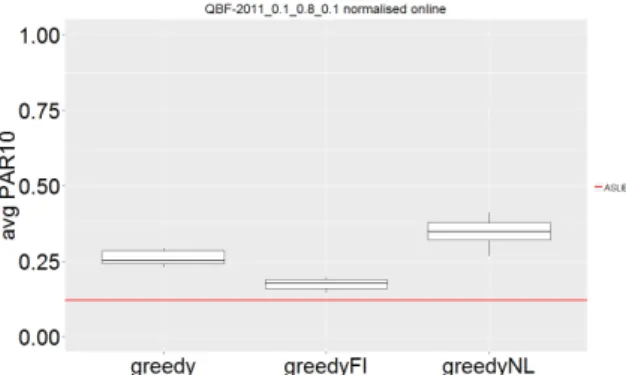
Figure 2: Boxplot summarising the answer to the question ’Is active learning useful?’. The presented data is collected during the online phase
Note that the Greedy-full-information strategy does not provide a real upper bound: it is possible to perform better than this strategy as more information is not guaranteed to always result in better predictions.
The plot with the results of the online phase is presented in figure 2. Online learning appears to be useful as the greedy strategy outperforms the greedy-no-learning strat-egy. The good performance of the greedy-full-information strategy shows the value of having access to more infor-mation.
The performance reported in figure 2 is the average per-formance over all online instances. For the first online in-stance the performance of the greedy-no-learning strategy is equal to that of the greedy strategy that does learn, but for the last online instance the performance of the greedy strategy that does learn is expected to be better because it has access to more data. The performance reported in figure 2 is the average of these (most likely) increasing performances.
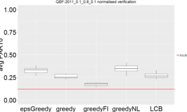
To quantify how much the greedy strategy has learned during the online phase, the quality of its predictions is tested on a set of verification instances. During the verifi-cation phase the models are no longer updated. The differ-ence in PAR10-score between the greedy strategy and the greedy-no-learning strategy is a measure for how much us-ing the online data improves the quality of the selection.
The plot with the results of the verification phase is presented in figure 3. Note that the performance of the greedy-full-information strategy is similar to the perfor-mance of llama. This is expected because the bench-mark performance was calculated using a 10-fold cross-validation where performance of models trained on 90% of the data is measured on the remaining 10%. The mod-els of the greedy-full-information strategy have also been trained on 90% of the data: 10% training data and 80% online data.
To answer the question titling this section: automatic online algorithm selection appears to be useful for the greedy approach.
Figure 3: Boxplot summarising the answer to the question ’Is active learning useful?’. The presented data is collected during the verification phase
4.3 Handling the Exploration vs. Exploitation Trade-off
When performing reinforcement learning one is typically faced with an exploration vs. exploitation trade-off. When no online learning is performed the predicted best algo-rithm is always selected because the only reason for se-lecting an algorithm is solving the next instance as well as possible. In an online learning setting a second reason for selecting an algorithm surfaces: additional informa-tion will be obtained and this informainforma-tion will increase the quality of future decisions.
Two exploration-incorporating strategies are compared to the simple greedy approach: ε-greedy (epsGreedy on the plots) and lower confidence bound (LCB on the plots). See section 2.4 for a description of these two strategies.
A first test is to compare each strategy’s performance during the online phase. This measures their ability to solve the exploration vs. exploitation trade-off: do they manage to benefit from exploring more by obtaining a bet-ter average performance?
The plot with the results of the online phase is presented in figure 4. The answer appears to be negative: explicit exploration does not result in a better average performance than greedy and theε-greedy strategy even drops down to the level of the greedy-no-learning strategy.
A second test is to check whether the exploration strate-gies managed to learn better models than the greedy strat-egy by comparing their performance on the verification data. If the exploration strategies managed to learn better models they have merit as they traded off some exploita-tion in favour of useful exploraexploita-tion. If this is not the case the exploration was not useful and simply resulted in pick-ing inferior algorithms without any noticeable gain.
The plot with the results of the verification phase is presented in figure 5. Exploration does not appear to have been useful as the models learned by theε-greedy and lower confidence bound strategy do not outperform the model learned by the greedy strategy. Note however that the additional information obtained during the on-line phase does result in better models than the
greedy-Figure 4: Boxplot summarising the answer to the ques-tion ’is explicit exploraques-tion useful?’. The presented data is collected during the online phase
Figure 5: Boxplot summarising the answer to the ques-tion ’is explicit exploraques-tion useful?’. The presented data is collected during the verification phase
no-learning strategy for all learning strategies.
5
Discussion and future work
The automatic online algorithm selection method pre-sented in section 2.2 is inefficient. Every time a new datapoint is collected for an algorithm, the corresponding regression model is retrained from scratch using all pre-vious data and the newly obtained datapoint. If the fit-ting of a model takes a long time this approach can be-come prohibitively expensive, especially if its complexity is influenced heavily by the amount of instances, as for each online instance a new model is trained and the mod-els are trained based on an ever increasing amount of in-stances. Identifying and implementing more efficient up-dating strategies is future work. Mondrian forests [18] for example are an online version of random forests that could be useful in this context.
There might be a theoretical problem with the proposed automatic online algorithm selection method. During the online phase an algorithm’s regression model is extended only with datapoints for which the algorithm was predicted to be best. Hence the new datapoints are all clustered in the same region(s) of the problem domain. Note also that
the region(s) where an algorithm is best is likely to change slightly every time a new instance is handled, as with the changing of an algorithm’s regression model all points in the domain where the algorithm’s predicted performance was better than that of another algorithm’s are likely to move slightly. Then again, in a sense the property that datapoints are mostly collected in the area where an algo-rithm is expected to be best is desirable. Knowing with high accuracy how poorly an algorithm performs on in-stances where it is bad is useless in this context whereas accurate predictions on instances for which the algorithm is likely to be one of the best are very relevant. However, note that predicting performance accurately is not the goal itself. What is important is that the actual best algorithm is the algorithm with predicted best score. The selection mapping does not change if a fixed value is added to each performance prediction.
At the start of this project it was thought that the explicit exploration would be useful. Current and future work is in-vestigating why this does not appear to be the case. There are two main hypotheses.
The first hypothesis is that the amount of exploration data collected during the online phase is negligible com-pared to the data gathered during the training phase, thus the influence of the exploration cannot be observed. A training set of 100 instances for 5 algorithms can be seen as a combination of 100 greedy choices and 400 explo-rative choices. The epsilon greedy strategy will explore 5% of the time, resulting in on average 50 new explorative datapoints during an online phase of 1000 instances. This hypothesis is currently being investigated
The second hypothesis is that exploration is already implicitly performed by the greedy strategy, rendering additional explicit exploration unnecessary. The greedy method is greedy in the sense that it always selects the best algorithm, but which the best algorithm is depends from instance to instance, thus over time performance dat-apoints for all algorithms are collected. In this way the greedy strategy implicitly explores. Investigating this hy-pothesis is future work.
In order to better quantify the improvements realised during the online phase, future work is to investigate the way in which the selection model improves in detail, by not only evaluating the overall models before and after the online phase, but also at several points during the online phase and by also dropping down a level and investigating how the individual regression models (one for each algo-rithm) evolve over time.
In future work the overhead of retraining the models should be explicitly considered and quantified in order to be able to quantify the net improvement of using the on-line data. In the experiments here reported this overhead is ignored.
An interesting path for future work is te develop an gorithm that learns how to perform automatic online al-gorithm selection form scratch, without any training data whatsoever. A straightforward initial methodology would
be to perform random or round-robin selection until suf-ficient samples have been collected for each algorithm to construct a regression model. Interesting challenges would be to include the option to add new algorithms at runtime and even identifying which kind of instances are hard for all algorithms, thereby inspiring the development of a new algorithm that performs well on these instances which can then be added to the system.
Other future work consists of implementing solu-tion strategies specifically designed for the contextual multi-armed bandit problem which are more theoretically founded, for example LinUCB [7].
6
Conclusions
A reinforcement learning methodology for automatic on-line algorithm selection has been introduced. It is limited to automatic algorithm selection methods based on perfor-mance predictions for each individual algorithm. It has been shown experimentally that the method is capable of learning from online data and thereby improves on auto-matic offline algorithm selection methods.
It has been shown that automatic online algorithm selec-tion can be modelled as a contextual multi-armed bandit problem.
A total of three solution strategies have been imple-mented and empirically tested: an approach that always greedily selects the best algorithm and two approaches that perform exploration: ε-greedy and lower confidence bound. The experiments suggest that the greedy strategy outperforms the explorative strategies.
Acknowledgements
Work supported by the Belgian Science Policy Office (BELSPO) in the Interuniversity Attraction Pole COMEX. (http://comex.ulb.ac.be).
The computational resources and services used in this work were provided by the VSC (Flemish Supercomputer Center), funded by the Research Foundation - Flanders (FWO) and the Flemish Government – department EWI
References
[1] P. Auer, N. Cesa-Bianchi, and P. Fischer. Finite-time anal-ysis of the multiarmed bandit problem. Machine learning, 47(2-3):235–256, 2002.
[2] B. Bernd. mlr: A new package to conduct machine learning experiments in r.
[3] B. Bischl, P. Kerschke, L. Kotthoff, M. Lindauer, Y. Mal-itsky, A. Fréchette, H. Hoos, F. Hutter, K. Leyton-Brown, K. Tierney, et al. Aslib: A benchmark library for algorithm selection.arXiv preprint arXiv:1506.02465, 2015. [4] B. Bischl, M. Lang, O. Mersmann, J. Rahnenführer, and
C. Weihs. BatchJobs and BatchExperiments: Abstraction mechanisms for using R in batch environments. Journal of Statistical Software, 64(11):1–25, 2015.
[5] B. Bischl, O. Mersmann, H. Trautmann, and M. Preuss. Al-gorithm selection based on exploratory landscape analysis and cost-sensitive learning. InGenetic and Evolutionary Computation Conference (GECCO), 2012.
[6] P. B. Brazdil, C. Soares, and J. P. Da Costa. Ranking learn-ing algorithms: Uslearn-ing ibl and meta-learnlearn-ing on accuracy and time results.Machine Learning, 50(3):251–277, 2003. [7] W. Chu, L. Li, L. Reyzin, and R. E. Schapire. Contex-tual bandits with linear payoff functions. InInternational Conference on Artificial Intelligence and Statistics, pages 208–214, 2011.
[8] V. A. Cicirello and S. F. Smith. The max k-armed bandit: A new model of exploration applied to search heuristic se-lection. InAAAI, pages 1355–1361, 2005.
[9] H. Degroote and P. De Causmaecker. Towards a knowl-edge base for performance data: A formal model for per-formance comparison. InProceedings of the Companion Publication of the 2015 on Genetic and Evolutionary Com-putation Conference, pages 1189–1192. ACM, 2015. [10] T. Doan and J. Kalita. Selecting machine learning
algo-rithms using regression models. In 2015 IEEE
Interna-tional Conference on Data Mining Workshop (ICDMW),
pages 1498–1505. IEEE, 2015.
[11] M. Gagliolo and J. Schmidhuber. Learning dynamic al-gorithm portfolios. Annals of Mathematics and Artificial Intelligence, 47(3-4):295–328, 2006.
[12] M. Gagliolo and J. Schmidhuber. Algorithm selection as a bandit problem with unbounded losses. In Interna-tional Conference on Learning and Intelligent Optimiza-tion, pages 82–96. Springer, 2010.
[13] B. A. Huberman, R. M. Lukose, and T. Hogg. An Eco-nomics Approach to Hard Computational Problems. Sci-ence, 275(5296):51–54, 1997.
[14] F. Hutter, L. Xu, H. H. Hoos, and K. Leyton-Brown. Algo-rithm runtime prediction: Methods & evaluation.Artificial Intelligence, 206:79–111, 2014.
[15] S. Kadioglu, Y. Malitsky, A. Sabharwal, H. Samulowitz, and M. Sellmann. Algorithm selection and scheduling. InPrinciples and Practice of Constraint Programming–CP 2011, pages 454–469. Springer, 2011.
[16] L. Kotthoff. Llama: leveraging learning to automatically manage algorithms.arXiv preprint arXiv:1306.1031, 2013. [17] L. Kotthoff. Algorithm Selection for Combinatorial Search
Problems: A Survey.AI Magazine, 35(3):48–60, 2014. [18] B. Lakshminarayanan, D. M. Roy, and Y. W. Teh.
Mon-drian forests: Efficient online random forests. InAdvances in Neural Information Processing Systems, pages 3140– 3148, 2014.
[19] A. Liaw and M. Wiener. Classification and regression by randomforest.R news, 2(3):18–22, 2002.
[20] Y. Malitsky, A. Sabharwal, H. Samulowitz, and M. Sell-mann. Non-model-based algorithm portfolios for sat. In
Theory and Applications of Satisfiability Testing-SAT 2011, pages 369–370. Springer, 2011.
[21] T. Messelis and P. De Causmaecker. An automatic al-gorithm selection approach for the multi-mode resource-constrained project scheduling problem.European Journal of Operational Research, 233(3):511–528, 2014.
[22] E. Nudelman, K. Leyton-Brown, H. H. Hoos, A.
De-vkar, and Y. Shoham. Understanding random sat: Be-yond the clauses-to-variables ratio. InPrinciples and Prac-tice of Constraint Programming–CP 2004, pages 438–452. Springer, 2004.
[23] J. R. Rice. The algorithm selection problem. Advances in Computers, 15:65–118, 1976.
[24] K. A. Smith-Miles. Cross-disciplinary perspectives on meta-learning for algorithm selection. ACM Computing Surveys (CSUR), 41(1):6, 2009.
[25] L. Xu, F. Hutter, H. Hoos, and K. Leyton-Brown. Evaluat-ing component solver contributions to portfolio-based algo-rithm selectors. InTheory and Applications of Satisfiability Testing–SAT 2012, pages 228–241. Springer, 2012. [26] L. Xu, F. Hutter, J. Shen, H. H. Hoos, and K.
Leyton-Brown. Satzilla2012: Improved algorithm selection based on cost-sensitive classification models.Proceedings of SAT Challenge, pages 57–58, 2012.