A Proportion-Based Selection Scheme for
Multi-objective Optimization
Liuwei Fu
School of Information Engineering Xiangtan University Xiangtan 411105, China Email: [email protected]
Juan Zou
(Corresponding author)
School of Information EngineeringXiangtan University Xiangtan 411105, China Email: [email protected]
Shengxiang Yang
School of Information EngineeringXiangtan University Xiangtan 411105, China
School of Computer Science and Informatics De Montfort University
Leicester LE1 9BH, U.K. Email: [email protected]
Gan Ruan
School of Information Engineering Xiangtan University Xiangtan 411105, China Email: [email protected]
Zhongwei Ma
School of Information Science and Engineering Central South University
Changsha 410083, China Email: mzw [email protected]
Jinhua Zheng
School of Information Engineering Xiangtan University Xiangtan 411105, China Email: [email protected]
Abstract—Classical multi-objective evolutionary algorithms (MOEAs) have been proven to be inefficient for solving multi-objective optimizations problems when the number of multi-objectives increases due to the lack of sufficient selection pressure towards the Pareto front (PF). This poses a great challenge to the design of MOEAs. To cope with this problem, researchers have developed reference-point based methods, where some well-distributed points are produced to assist in maintaining good diversity in the optimization process. However, the convergence speed of the population may be severely affected during the searching procedure. This paper proposes a proportion-based selection scheme (denoted as PSS) to strengthen the convergence to the PF as well as maintain a good diversity of the population. Computational experiments have demonstrated that PSS is sig-nificantly better than three peer MOEAs on most test problems in terms of diversity and convergence.
I. INTRODUCTION
Many real world application problems are multi-objective optimization problems (MOPs), which include multiple con-flicting objectives that must be optimized simultaneously. In the evolutionary multi-objective optimization (EMO) com-munity, multi-objective optimization evolutionary algorithms (MOEAs) have benn demonstrated to be effective in solving these problems [1]-[4]. So far, many different EMO algorithms have been developed, such as Pareto-based methods, e.g., NSGA-II [5], SPEA2 [6], decomposition-based approaches, e.g., MOEA/D [7], and indicator-based approaches [8, 9], e.g., HypE [10], SMS-EMOA [11]. However, Pareto-based algorithms more or less lose selection pressure to the PF in the optimization process when solving problems having more than three objectives, i.e., many-objective optimization problems (MaOPs). As a result, the whole performance of MOEAs can be affected by the decrease of convergence.
Pareto-based approaches compare solutions according to their dominance relation and density. The nondominated in-dividuals are considered as primarily selected solutions. How-ever, the Pareto-based dominance relationship has encountered great difficulties in MaOPs when the number of obectives in-creases [12, 13, 14]. Therefore, some researchers have focused on modifying the dominance relation to provide sufficient selection pressure towards the PF. Many improved methods have been proposed, such as SPEA2+SDE [15],-dominance [16, 17], and fuzzy Pareto dominance [18-24].
Indicator-based approaches use a single performance indi-cator to guide the search during the evolutionary process. The indicator-based EA (IBEA) [25] is a pioneer in this group. Recently, the hypervolume [26], Two Arch2 [27] and S metric selection evolutionary algorithm [28] have been proposed. Indicator-based approaches have been demonstrated to be effective in balancing convergence and diversity due to their good theoretical properties. Nevertheless, the computational cost of the used metrics, e.g., hypervolume, grows exponen-tially with an increase in the number of objectives [29].
Decomposition-based methods decompose a problem with multiple objectives into a set of single-objective subproblems, which are then optimized simultaneously using evolutionary algorithms. The diversity of population is maintained by a set of pre-defined well-distributed reference points. The per-pendicular distance between the individual and the reference line is usually used in reference vector-based decomposition methods. Reference lines are obtained by connecting reference points and the origin. Consequently, the convergence speed is affected by the perpendicular distance-based method to some degree, although these methods can balance convergence and diversity.
To handle these problems, the perpendicular distance must be replaced with the Euclidean distance to strengthen the selection pressure. In this paper, we propose a proportion-based selection scheme (PSS) for multi-objective optimization, where those solutions having the most approximate proportion can be obtained, thereby maintaining the diversity of the population. The center point (CR) of the reference set is calculated using the average value of all reference points on each objective. The distance from the reference point to the center point is also uniformly-distributed. Therefore, we can use the proportion to find uniformly-distributed Pareto optimal solutions. The proportion-based method is different from Pareto-based approaches and indicator-based approaches, but it is similar to reference point-based MOEAs.
The remainder of this paper is organized as follows. Section II presents the background information on reference point-based algorithms. The proposed PSS is described in detail in Section III. Experimental studies on well-known test problems are carried out in Section IV. Finally, conclusions are drawn in Section V.
II. PRELIMARIES
In this section, basic definitions in this paper are first given. Then, we briefly introduce the original MOEA/D and NSGA-III.
A. Basic Definitions
Perpendicular distance, euclidean distance, direction vector and proportion are defined as follows:
Definition 1: The distance between an individual and the centroid line is called the perpendicular distance, where a centroid line is defined by joining the centroid point with the origin.
Definition 2:The distance from an individual to the centroid is called the euclidean distance.
Definition 3: AP~ is the direction vector of individual P, whereAis the projective point of individualP on the centroid line.
Definition 4: The perpendicular distance of each individual is calculated, denoted by D. The proportion P of each individual is described as follows:
Pj=
Dj
max(D1, D2, . . . , Dn)
, (1)
wherej is the j th individual of the population.
B. MOEA/D and NSGA-III
The key idea of MOEA/D is to use a predefined set of well-distributed weight vectors to maintain the diversity of the new population. Each subproblem can find the best solution by using the aggregate function in the population. The collection of the solution on each well-distributed weight vector can be viewed as an approximation of the true PF. Generally, there are three aggregation functions: the weighted sum, Chebyshev, and penalty-based boundary intersection (PBI) function in MOEA/D. Let us take the PBI as an example. We suppose
Algorithm 1 Framework of PSS 1: Λ←GenerateReferencePoints() 2: P0 ←InitializePopulation() 3: RP ←ComputeProportion(Λ) 4: RV ←ObtainVector(Λ) 5: t←0
6: whilethe termination criterion is not metdo
7: Qt ←MakeOffspringPopulation(Pt) 8: St←Pt∪Qt 9: SP ←ComputeProportion(St) 10: SV ←ObtainVector(St) 11: κ←Associate(St,Λ, RP, RV, SP, SV) 12: Pt+1 ←Niching(κ) 13: end while Algorithm 2 GetCentriod(PopulationSt) Require: PopulationSt
Ensure: C(The centroid of reference set or population set) 1: fori= 1tomdo 2: Ci ←0 3: forj= 1to ndo 4: Ci ←Ci+St[j][i] 5: end for 6: Ci =Ci/n 7: end for
w1, w2, . . . , wn is a set of evenly spread weight vectors, then
each subproblem is optimized respectively by: P BI(x, wj) =d1+θd2
where j = 1,2, . . . , N, wj = (wj1, wj2, . . . , wjm)T, d1 is
the distance from the individual to the origin, d2 is the
per-pendicular distance between the individual in the population and each of the reference lines wj, and θ is the penalized
parameter. Each individual x∗ of the population can find a reference vector according to the PBI value. MOEA/D can work well for the curve shape friendly of the Pareto-optimal front.
The III framework is similar to the original NSGA-II except in its selection mechanism, and the diversity of a population is maintained by a set of well-distributed reference vector. Further details of NSGA-III can be found in references [30, 31].
III. PROPOSEDPSS ALGORITHM
The framework of the proposed PSS algorithm is described in Algorithm 1. In line 1, we use Das and Denis’s systematic approach [32] to generate a set of N reference points, denoted as Λ = {λ1, λ2, . . . , λN}. λj (j = 1,2, . . . , N) is an m
-dimensional vector for anm-objective problem. Line 2 denotes that the initial population P0 with N members is randomly
produced. The proportion of the reference point (RP) is initialized in line 3. The centroid point of the reference set is calculated in Algorithm 2. The perpendicular distance of each reference point from the centroid line is calculated. Then, the proportion is the value of perpendicular distance to maximum value of perpendicular distance. In line 4, the perpendicular direction (RV) from the projection point of reference point
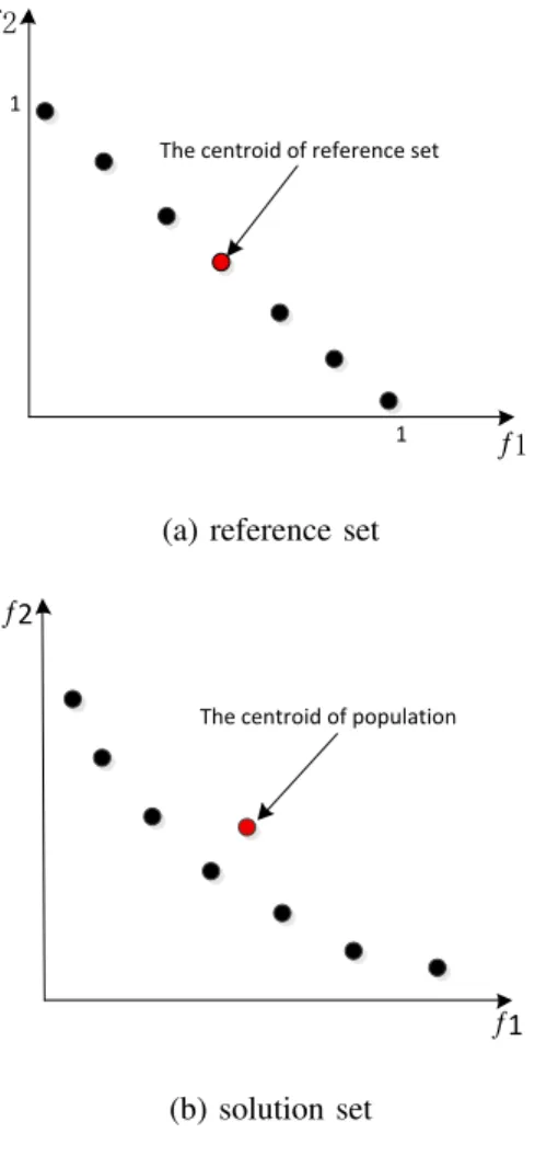
1 1
The centroid of reference set
ƒ2
ƒ1 (a) reference set
The centroid of population
ƒ1 ƒ2
(b) solution set Fig. 1. The centroid points.
to reference point is initialized. Lines 6-13 are iterated until the termination criterion is satisfied. The offspring population Qt, having N members, was created from Pt by using the
recombination operator and mutation operator in line 7. Then, the new populationStis the combination of populationP and
Qin line 8. Lines 9-10 denote that each individual’s proportion and direction vector can be obtained in the same way as Lines 3-4. In line 11, the function associate is used to split the members in St into a set ofN niche, κ={κ1, κ2, . . . , κN}.
In addition, each reference point is allocated to a niche. In Line 12, the new population, Pt+1, is filled with individuals
produced by the niche operator. In this paper, proportion is the key concept in PSS.
In the following sections, the important procedures of PSS are described in detail.
A. The Centroid of Reference Set and Population Set
In Fig. 1 (a), CR is the centroid of the reference set and Nr is the size of the reference set. Then, each objective value
Dr
1 1 The centroid of reference set
ƒ1 ƒ2 Dr 𝑃𝑟𝑗= 𝐷𝑟𝑗 max(𝐷𝑟1, 𝐷𝑟2, … , 𝐷𝑟𝑛)
Fig. 2. The proportion of the reference point.
of CRis calculated by the following formula: CR(i) = 1 Nr Nr X j=1 Rji, (2)
wherei= (1,2, . . . , m), and m is the number of objectives, j= (1,2, . . . , Nr), andRji is the value of thej-th reference
point in thei-th objective.
Similarly, in Fig. 1 (b),CSis the centroid of the population set, and Ns is the size of the population set. Then, each
objective value ofCS is obtained by the following formula: CS(i) = 1 Ns Ns X j=1 Sji, (3)
whereSji is the value ofj-th individual of the population in
the i-th objective. The procedure of calculating the centroid of the population or reference set is presented in Algorithm 2.
B. The Proportion of Reference Set and Population Set
We define a centroid line corresponding to the centroid point by joining the centroid point with the origin. The perpendicular distance (denoted asDr) of each reference point is calculated. Finally, the proportion of each reference point in the reference set is computed by the following formula:
P rj=
Drj
max(Dr1, Dr2, . . . , Drn)
, (4)
where P rj is the proportion of the j-th reference point to
the centroid point.Drj is the perpendicular distance from the
reference point to the centroid point of the reference set. This is illustrated in Fig. 2.
Similarly, in Fig. 3, the proportion of each individual in the solution set (P s) is computed by the following formula:
P sj=
Dsj
max(Ds1, Ds2, . . . , Dsn)
, (5)
where Dsj is the perpendicular distance from the j-th
indi-vidual to the centroid point of the solution Set. The procedure is presented in Algorithm 3.
Ds Ds The centroid of population
ƒ1 ƒ2
𝑃𝑠𝑗= 𝐷𝑠𝑗 max(𝐷𝑠1, 𝐷𝑠2, … , 𝐷𝑠𝑛)
Fig. 3. The proportion of solutions in the population.
Algorithm 3 ComputeProportion(Population St)
Require: The PopulationSt
Ensure: Proportion set(P) 1: C←GetCentriod(St) 2: fori= 1toN do
3: Di= Perpendicular distance between the reference point (or
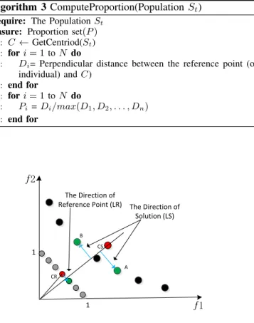
individual) andC) 4: end for 5: fori= 1toN do 6: Pi=Di/max(D1, D2, . . . , Dn) 7: end for 1 1 The Direction of
Reference Point (LR) The Direction of Solution (LS) CS ƒ1 ƒ2 CR A B
Fig. 4. The direction of the reference point and population set.
C. The Direction of Reference point and Solution point
In Fig. 4, suppose solutionA,Bis similar to reference point rin that they have similar proportions.Ais a best solution for the reference pointr, butBis a bad one. Therefore, we use the cosine similarity to select the individual in the population, the bigger the value of cosine similarity, the greater the selected chance that the individual is chosen. we define the direction vector of each reference point (Dr~ )by joining the reference point with the centroid line of the reference set. the direction vector of each individual in the population (Ds~ ) by joining
1 1 R CS ƒ1 ƒ2 A B C CR
Fig. 5. Association of population members with reference points is illustrated.
Algorithm 4 Associate(R,St,RP,RV,SP,SV)
Require: R(Reference Set),St(Population Set),RP (Proportion of
Reference point),RV (Direction Vector of Reference point),SP
(Proportion of Individual),SV (Direction Vector of Individual),
N r(Size of the Reference Set),N s(Size of the population set)
Ensure: κ
1: fori= 1 toN rdo
2: κi ←0
3: forj= 1to N sdo
4: κi select the individual that makeRPi−SPj minimum
and cosine maximum, simultaneously
5: end for
6: end for
the individual with the centroid line of the population. The value of cosine is computed by two direction vectors:
cosα= ~ Dr ~Ds
|Dr~ ||Ds~ | (6)
D. Association Operation
After the proportion was computed based on the centroid point, next we need toassociateeach population member with a reference point. The reference point whose proportion and cosine is equal to a population member in the objective space is considered associated with the population member. This is illustrated in Fig. 5. For a reference point R, individuals A, B and C are selected because they have the approximation of proportion and cosine according to the proportion and cosine ofR. The procedure is presented in Algorithm 4. Each member of the reference point will associate with one or more individuals in the population.
E. Selection Mechanism
Each reference point could be associated with one or multi-ple solutions in the population according to the proportion and cosine values of the reference point. Thus, we select an individual with the shortest Euclidean distance between the reference point and associated individual. The results are presented in Fig. 6. For a reference pointR, the individualB
1 1 R ƒ1 ƒ2 A B C :Discarded individual :Selected individual
Fig. 6. Niche preservation.
Algorithm 5 Niching(R,κ)
Require: R(Reference Set),κ, Nr is the number of reference set, Ns is the number of population set
Ensure: Pt+1 1: k= 0 2: fori= 1toNr do 3: ifsize(κi) == 1then 4: Pt+1=Pt+1∪s(s ∈κi) 5: end if 6: ifsize(κi)>=1then
7: Pt+1=Pt+1∪s(s∈κi&&s have the shortest Euclidean
distance)
8: end if
9: k+ + 10: end for
11: whilek < Ns do
12: Pt+1=Pt+1∪s(s∈κRandom()) &&s have the shortest
Euclidean distance)
13: end while
is selected because it has the shortest Euclidean distance from R, but individuals A and B are discarded. The procedure is presented in Algorithm 5.
IV. EXPERIMENTAL STUDIES
A. Experimental Setup
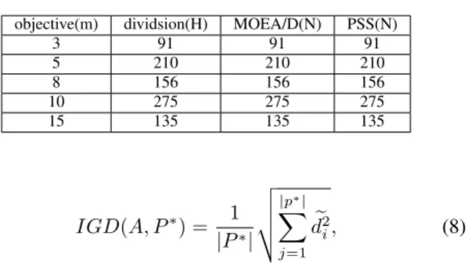
The five test instances DTLZ1-5 [33] are used as test functions. In each instance, there were 3, 5, 6, 8, 10, and 15 objectives. These test problems have a variety of characteris-tics and different PFs. In order to evaluate the performance of algorithms, we used the generational distance (GD) [34], inverted generational distance (IGD) [35] metrics to evaluate the proposed method. We obtained the final points in the objective space and called them set A; P* is a set of uniformly distributed points along the PF. The metrics GD and IGD are defined as follows: GD(A, P∗) = 1 |A| v u u t |A| X j=1 d2 i (7) TABLE I THE POPULATION SIZE
objective(m) dividsion(H) MOEA/D(N) PSS(N)
3 91 91 91 5 210 210 210 8 156 156 156 10 275 275 275 15 135 135 135 IGD(A, P∗) = 1 |P∗| v u u t |p∗| X j=1 e d2 i, (8)
where di(dei) is the Euclidean distance between the i-th
member in the set A(P∗) and its nearest member in the Set
P∗(A). GD can measure the convergence of the obtained
solutions. IGD is a comprehensive indicator, which evaluates the convergence and diversity of solutions.
We compared three other original algorithms MOEAs, SPEA2+SDE, IBEA and MOEA/D to PSS. The population size N in each algorithm is listed in Table I, where N = Cm
H+m−1−1 and H is the number of divisions considered
along each objective axis. The population size of the original SPEA2+SDE is 100. The Wilcoxon ranksum test [36] was carried out to indicate the significance between different results at the 0.05 significance level.
B. Comparison Results
In this subsection, the comparison results among PSS, SPEA2+SDE, IBEA and MOEA/D are presented. The mean GD and IGD values of each compared algorithm for DTLZ1-5 problems are provided in Table II, where the best performance is shown in bold.
From Table II, PSS is better than SPEA2+SDE, IBEA and MOEA/D-PBI on most DTLZ1 except 8- and 10-objective instances. Additionally, for DTLZ2, PSS outper-forms SPEA2+SDE, IBEA and MOEA/D on all instances. For DTLZ3, PSS is a little worse than SPEA2+SDE and IBEA. PSS is better than SPEA2+SDE, IBEA on DTLZ4, DTLZ5. However, PSS is little worse than MOEA/D-PBI on DTLZ5. The GD metric purely presents the convergence of an algorithm, it indicates that PSS has the best convergence performance among the four algorithms.
PSS performed better than SPEA2+SDE, IBEA and MOEA/D on most tested problems in terms of the IGD metric. It outperformed SPEA2+SDE, IBEA and MOEA/D on DTLZ4 except for problems with 15 objectives. As for DTLZ1, only PSS was worse than SPEA2+SDE and IBEA on 5-objective and 8-objective instances. In addition, PSS had the smaller IGD value than SPEA2+SDE, IBEA and MOEA/D in DTLZ2, DTLZ3, DTLZ4, DTLZ5 on most objective instances. Since the IGD metric can reflect the comprehensive performance of algorithms in terms of convergence and diversity, it can be concluded that PSS shows the best convergence and diversity on most problems.
TABLE II
RESULTS OF THEGDANDIGDVALUES FOR FOUR ALGORITHMS WITH VARYING NUMBER OF OBJECTIVESm,WHERE THE AVERAGE OVER30 INDEPENDENT RUNS IS SHOWN
Problems m GD IGD
PSS SPEA2+SDE IBEA MOEA/D-PBI PSS SPEA2+SDE IBEA MOEA/D-PBI
DTLZ1
3 2.097425E-4 2.498871E-4‡ 2.151756E-4† 2.132740E-4‡ 1.870439E-2 2.091488E-2‡ 2.404065E-2‡ 1.871996E-2‡
5 1.825690E-3 2.140118E-3‡ 1.795267E-3 1.852401E-3‡ 6.180973E-2 6.015305E-2 6.474986E-2‡ 6.194315E-2‡ 8 3.822195E-3 4.745083E-3‡ 4047640E-3‡ 3.804577E-3 1.091299E-1 9.712204E-2‡ 9.699570E-2 1.089212E-1‡ 10 4.749049E-3 6.023592E-3‡ 5.200348E-3‡ 4.741181E-3 9.958144E-2 1.152702E-1‡ 1.116092E-1‡ 9.647347E-2
15 4.327403E-3 7.654410E-3‡ 6.822330E-3‡ 5.078567E-3‡ 1.620598E-1 1.427370E-1‡ 1.296625E-1 1.401267E-1‡
DTLZ2
3 2.446136E-6 2.379738E-4‡ 6.349680E-5‡ 3.647608E-5‡ 5.009597E-2 7.222258E-2‡ 8.333383E-2‡ 5.015115E-2‡
5 2.193702E-5 4.342490E-4‡ 2.824714E-4‡ 2.501673E-4‡ 1.569619E-1 1.838502E-1‡ 1.854146E-1‡ 1.582530E-1‡
8 3.375279E-5 4.147951E-4‡ 5.951524E-4‡ 3.777484E-4‡ 4.466976E-1 4.663982E-1‡ 4.710770E-1‡ 4.512431E-1‡
10 1.268159E-4 3.344294E-4‡ 6.844971E-4‡ 9.913873E-4‡ 4.285472E-1 5.608170E-1‡ 5.562808E-1‡ 4.221368E-1
15 1.117240E-4 3.555315E-4‡ 7.645812E-4‡ 5.017912E-4‡ 6.495836E-1 6.816699E-1‡ 6.689002E-1‡ 6.764107E-1‡
DTLZ3
3 1.296890E-2 2.408237E-4 5.313469E1‡ 4.374955E-4‡ 1.325862E-1 7.077331E-2‡ 2.221019E2‡ 5.066953E-2 5 4.506600E-3 5.619237E-4‡ 4.078149E-4 6.126329E-4† 1.753776E-1 1.872975E-1‡ 1.828076E-1‡ 1.592967E-1 8 1.892800E-3 6.235349E-4† 8.203467E-4† 3.264915E-4 4.503561E-1 4.821155E-1‡ 4.889935E-1‡ 7.273809E-1‡ 10 5.189649E-3 7.992748E-4 2.027073E-2† 1.536804E-3‡ 4.261625E-1 5.929791E-1‡ 5.838285E-1‡ 6.810744E-1‡ 15 1.789564E-3 8.062062E-4† 9.103727E-3‡ 2.550453E-4 6.564342E-1 7.207506E-1‡ 7.124582E-1‡ 1.004235‡
DTLZ4
3 1.659870E-6 1.488738E-4‡ 1.512529E-3† 8.394296E-5‡ 5.012796E-2 2.671447E-1‡ 5.966096E-1‡ 5.029633E-2‡
5 2.522474E-5 4.152005E-4‡ 1.143932E-3‡ 1.373303E-4† 1.576663E-1 3.316153E-1‡ 2.539851E-1‡ 5.090315E-1‡
8 3.385892E-5 5.664861E-4‡ 5.563174E-4‡ 8.892509E-5† 4.558352E-1 4.813135E-1† 4.720429E-1‡ 7.129017E-1‡
10 1.897215E-4 5.300003E-4‡ 4.659565E-4‡ 1.320534E-4 4.434634E-1 5.645314E-1‡ 5.543840E-1† 7.292015E-1†
15 3.206397E-5 5.389029E-4‡ 1.302247E-3† 1.167799E-4‡ 6.566471E-1 6.823312E-1† 6.772528E-1† 9.082683E-1†
DTLZ5
3 6.461373E-4 3.649849E-5‡ 1.263669E-6 5.184335E-2‡ 2.666319E-2 8.122719E-3 1.144353E-2‡ 3.198290E-2‡
5 1.315031E-2 5.415597E-2‡ 6.448064E-2‡ 1.383002E-2† 3.005594E-2 5.979775E-2‡ 2.867739E-2 2.924760E-2‡
8 1.663207E-2 5.910784E-2‡ 7.500306E-2‡ 1.495193E-3 6.453904E-2 1.256837E-1‡ 5.042064E-2 6.724457E-2‡ 10 1.095402E-2 6.590729E-2‡ 8.104358E-2‡ 1.070695E-3 4.451275E-2 1.457291E-1‡ 6.667566E-2‡ 5.018808E-2‡ 15 6.629625E-3 7.129200E-2‡ 8.113172E-2‡ 6.811994E-9 1.528460E-1 1.536967E-1† 6.292434E-2 1.537017E-1‡ ‡ and † indicate PSS performs significantly better than and equivalently to the corresponding algorithm, respectively.
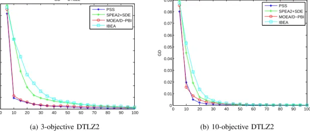
0 10 20 30 40 50 60 70 80 90 100 0 0.01 0.02 0.03 0.04 0.05 0.06 0.07 0.08 0.09 GD−−−DTLZ2 GD PSS SPEA2+SDE MOEA/D−PBI IBEA 0 10 20 30 40 50 60 70 80 90 100 0 0.01 0.02 0.03 0.04 0.05 0.06 0.07 0.08 0.09 GD−−−DTLZ2 GD PSS SPEA2+SDE MOEA/D−PBI IBEA
(a) 3-objective DTLZ2 (b) 10-objective DTLZ2
Fig. 7. The convergence regarding the GD metric of algorithms for DTLZ2 with 3-objective and 10-objective instances.
To verify the selection pressure toward PF, the polyline charts were drawn using the GD metric on 3-objective and 10-objective DTLZ2 instances. The four average GD val-ues were obtained by evaluating the former 100 generations of population, respectively. The four polyline, asterisk sign, plus sign, dot sign and rectangular sign, represent the PSS, SPEA2+SDE, MOEA/D and IBEA, respectively. In Fig. 7, for the DTLZ2 problem with 3 objectives, the convergence of PSS is better than SPEA2+SDE, IBEA and MOEA/D after
about 15-th generation, which shows that PSS has a faster convergence speed on some problems. In addition, for the 10-objective DTLZ2 problem, PSS also has better convergence performance than MOEA/D, IBEA and SPEA2+SDE.
The PSS had better performance than MOEA/D, IBEA, SPEA2+SDE on most problems. One of the important reasons for the PSS is due to their selection criterion that can improve the convergence of the algorithm. The selection mechanism in PSS uses the shortest Euclidean distance between the individ-ual of the solution and reference point to produce selection
pressure toward PF. In addition, the proportion method was used to maintain the diversity of the population.
V. CONCLUSION
This paper has proposed the PSS algorithm for multi-objective optimization. PSS aims to improve the selection pressure to maintain the convergence of the population in the selection mechanism. To attain this goal, the proportion-based selection mechanism is introduced into the proposed methods. From comparison results, PSS had the best performance com-pared to MOEA/D, IBEA and SPEA2+SDE on most instances. In the future, we will apply PSS to more practical problems.
ACKNOWLEDGMENT
This work was supported by the National Natural Sci-ence Foundation of China under Grant Nos. 61502408 and 61673331, the Education Department Major Project of Hunan Province under Grant No. 17A212615, the CERNET Innova-tion Project under Grant No. NGII20150302, and the Research Project on Teaching Reform of Colleges and Universities in Hunan (Network Construction and Auxiliary Teaching of Computer Culture Foundation).
REFERENCES
[1] G. Ruan, G. Yu, J. Zheng, J. Zou, and S. Yang, “The effect of diversity maintenance on prediction in dynamic multi-objective optimization,” Appl. Soft Comput., vol. 58, pp. 631-647, 2017.
[2] Z. Peng, J. Zheng, J. Zou, and M. Liu, “Novel prediction and memory strategies for dynamic multiobjective optimization,” Soft Comput., 2015, 19(9): 2633-2653.
[3] G. Yu, R. Shen, J. Zheng, M. Li, J. Zou, and Y. Liu, “Binary search based boundary elimination selection in many-objective evolutionary optimization,” Appl. Soft Comput., vol. 60, pp. 689-705, 2017. [4] J. Zheng, G. Yu, Q. Zhu, X. Li, and J. Zou, “On decomposition methods
in interactive user-preference based optimization,” Appl. Soft Comput., vol. 52, pp. 952-973, 2017.
[5] K. Deb, A. Pratap, S. Agarwal, and T. Meyarivan, “A fast and elitist mul-tiobjective genetic algorithm: NSGA-II,” IEEE Trans. on Evol. Comput., vol. 6, no. 2, pp. 182-197, 2002.
[6] Z. Eckart, L. Marco, and T. Lothar, “SPEA2: Improving the strength pareto evolutionary algorithm for multiobjective optimization,” in Proc. Evol. Methods for Design Optim. and Control with Appl. to Industrial Problems, 2001, pp. 95-100.
[7] Q. Zhang and H. Li, “MOEA/D: A multiobjective evolutionary algorithm based on decomposition,” IEEE Trans. on Evol. Comput., vol. 11, no. 6, pp. 712-731, 2007.
[8] C. A. C. Coello, “Evolutionary multi-objective optimization,” Wiley Interdisciplinary Reviews: Data Mining and Knowledge Discovery, vol. 1, no. 5, pp. 444-447, 2011.
[9] T. Wagner, N. Beume, and B. Naujoks, “Pareto-, aggregation-, and indicator-based methods in many-objective optimization,” in: Proc. Evol. Multi-Criterion Optim., 2007, pp. 742-756.
[10] J. Bader and E. Zitzler, “HypE: An algorithm for fast hypervolume-based many-objective optimization,” Evol. Comput., vol. 19, no. 1, pp. 45-76, 2011.
[11] B. Nicola, B. Naujoks, and M. Emmerich, “SMS-EMOA: Multiobjec-tive selection based on dominated hypervolume,” Europ. J. Oper. Res., vol. 181, no. 3, pp. 1653-1669, 2007.
[12] K. Ikeda, H. Kita, and S. Kobayashi, “Failure of Pareto-based MOEAs: Does non-dominated really mean near to optimal?” in Proc. 2001 IEEE Congr. Evol. Comput., vol. 2. Seoul, Korea, 2001, pp. 957-962. [13] V. Khare, X. Yao, and K. Deb, “Performance scaling of multi-objective
evolutionary algorithms,” in Proc. Evol. Multi-Criter. Optim., Faro, Por-tugal, 2003, pp. 376-390.
[14] R. C. Purshouse and P. J. Fleming, “Evolutionary many-objective opti-misation: An exploratory analysis,” in Proc. IEEE Congr. Evol. Comput., vol. 3, Canberra, Australia, 2003, pp. 2066-2073.
[15] M. Li, S. Yang, and X. Liu, “Shift-based density estimation for Pareto-based algorithms in many-objective optimization,” IEEE Trans. Evol. Comput., vol. 18, no. 3, pp. 348-365, Jun. 2014.
[16] M. Laumanns, L. Thiele, K. Deb, and E. Zitzler, “Combining conver-gence and diversity in evolutionary multiobjective optimization,” Evol. Comput., vol. 10, no. 3, pp. 263-282, 2002.
[17] K. Deb, M. Mohan, and S. Mishra, “Evaluating the-domination based multi-objective evolutionary algorithm for a quick computation of Pareto-optimal solutions,” Evol. Comput., vol. 13, no. 4, pp. 501-525, 2005. [18] M. Farina and P. Amato, “A fuzzy definition of ’optimality’ for
manycri-teria optimization problems,” IEEE Trans. Syst., Man, Cybern. A, Syst., Humans, vol. 34, no. 3, pp. 315-326, May 2004.
[19] M. K¨oppen, R. Vicente-Garcia, and B. Nickolay, “Fuzzy-Paretodominance and its application in evolutionary multi-objective optimization,” in: Proc. Evol. Multi-Criter. Optim., Guanajuato, Mexico, 2005, pp. 399-412.
[20] S. Yang, M. Li, and X. Liu, “A grid-based evolutionary algorithm for many-objective optimization,” IEEE Trans. Evol. Comput., vol. 17, no. 5, pp. 721-736, Oct. 2013.
[21] K. Li, Q. Zhang, S. Kwong, M. Li, and R. Wang, “Stable matching-based selection in evolutionary multiobjective optimization,” IEEE Trans. Evol. Comput., vol. 18, no. 6, pp. 909-923, Dec. 2014.
[22] K. Li, S. Kwong, J. Cao, “Achieving balance between proximity and di-versity in multi-objective evolutionary algorithm,” Inform. Sci., vol. 182, no. 1, pp. 220-242, 2012.
[23] J. Zou, Q. Li, S. Yang, H. Bai, and J. Zheng, “A prediction strategy based on center points and knee points for evolutionary dynamic multi-objective optimization,” Appl. Soft Comput., vol. 61, pp. 806-818, 2017. [24] J. Zou, J. Zheng, R. Shen, and C. Deng, “A novel metric based on changes in pareto domination ratio for objective reduction of many-objective optimization problems,” J. Exper. & Theoret. Art. Intell., vol. 29, no. 5, pp. 983-994, 2017.
[25] E. Zitzler and S. Kunzli. Indicator-Based Selection in Multiobjective Search. In Conference on Parallel Problem Solving from Nature (PPSN VIII), vol. 3242 of LNCS, pp. 832-842, 2004.
[26] E. Zitzler and L. Thiele, “Multiobjective evolutionary algorithms: A comparative case study and the strength Pareto approach,” IEEE Trans. Evol. Comput., vol. 3, no. 4, pp. 257-271, Nov. 1999.
[27] Wang, Handing, Licheng Jiao, and Xin Yao, “Two Arch2: An improved two-archive algorithm for many-objective optimization,” IEEE Trans. Evol. Comput., vol. 19, no. 4, pp. 524-541, 2015.
[28] N. Beume, B. Naujoks, and M. Emmerich, ‘SMS-EMOA: Multiobjective selection based on dominated hypervolume,” Eur. J. Oper. Res., vol. 181, no. 3, pp. 1653-1669, 2007.
[29] K. Bringmann and T. Friedrich, “Don’t be greedy when calculating hypervolume contributions,” in: Proc. 10th ACM SIGEVO Workshop Found. Genet. Algorithms, Orlando, FL, USA, 2009, pp. 103-112. [30] K. Deb and H. Jain, “An evolutionary many-objective optimization
algorithm using reference-point based non-dominated sorting approach, Part I: Solving problems with box constraints,” IEEE Trans. Evol. Comput., vol. 18, no. 4, pp. 577-601, Aug. 2014.
[31] H. Jain and K. Deb, “An evolutionary many-objective optimization algorithm using reference-point based nondominated sorting approach, part II: handling constraints and extending to an adaptive approach,” IEEE Trans. Evol. Comput., vol. 18, no. 4, pp. 602-622, 2014.
[32] I. Das and J. Dennis, “Normal-boundary intersection: A new method for generating the Pareto surface in nonlinear multicriteria optimization problems,” SIAM J. Optim., vol. 8, no. 3, pp. 631-657, 1998.
[33] K. Deb, L. Thiele, M. Laumanns, and E. Zitzler, “Scalable multiobjective optimization test problems,” Inst. Commun. Inf. Technol., ETH Zurich, Zurich, Switzerland, TIK Tech. Rep 112, 2001.
[34] D. A. Van Veldhuizen, “Multiobjective evolutionary algorithms: classifi-cations, analyses, and new innovations,” Tech. Report, DTIC Document, 1999.
[35] E. Zitzler, L. Thiele, M. Laumanns, C. M. Fonseca, and V. G. da Fon-seca, “Performance assessment of multiobjective optimizers: An analysis and review,” IEEE Trans. Evol. Comput., vol. 7, no. 2, pp. 117-132, Apr. 2003.
[36] F. Wilcoxon, “Individual comparisons by ranking methods,” Biom. Bull. vol. 1, no. 6, pp. 80-83, 1945.