University of Dundee
Tree-based Ensemble Classifier Learning for Automatic Brain Glioma Segmentation
Amiri, Samya; Ali Mahjoub, Mohamed; Rekik, Islem
Published in: Neurocomputing DOI: 10.1016/j.neucom.2018.05.112 Publication date: 2018 Document Version Peer reviewed version
Link to publication in Discovery Research Portal
Citation for published version (APA):
Amiri, S., Ali Mahjoub, M., & Rekik, I. (2018). Tree-based Ensemble Classifier Learning for Automatic Brain Glioma Segmentation. Neurocomputing, 313, 135-142. https://doi.org/10.1016/j.neucom.2018.05.112
General rights
Copyright and moral rights for the publications made accessible in Discovery Research Portal are retained by the authors and/or other copyright owners and it is a condition of accessing publications that users recognise and abide by the legal requirements associated with these rights.
• Users may download and print one copy of any publication from Discovery Research Portal for the purpose of private study or research. • You may not further distribute the material or use it for any profit-making activity or commercial gain.
• You may freely distribute the URL identifying the publication in the public portal.
Take down policy
If you believe that this document breaches copyright please contact us providing details, and we will remove access to the work immediately and investigate your claim.
Tree-based Ensemble Classifier Learning for Automatic
Brain Glioma Segmentation
Samya Amiri
LATIS lab, ENISo – National Engineering School of Sousse, Tunisia
Mohamed Ali Mahjoub
LATIS lab, ENISo – National Engineering School of Sousse, Tunisia
Islem Rekik∗
BASIRA lab, CVIP group, School of Science and Engineering, Computing, University of Dundee, UK
Abstract
We introduce a dynamic multiscale tree (DMT) architecture that learns how to leverage the strengths of different state-of-the-art classifiers for supervised multi-label image segmentation. Unlike previous works that simply aggregate or cascade classifiers for addressing image segmentation and labeling tasks, we propose to embed strong classifiers into a tree structure that allows bi-directional flow of information between its classifier nodes to gradually improve their per-formances. Our DMT is a generic classification model that inherently embeds different cascades of classifiers while enhancing learning transfer between them to boost up their classification accuracies. Specifically, each node in our DMT can nest a Structured Random Forest (SRF) classifier or a Bayesian Network (BN) classifier. The proposed SRF-BN DMT architecture has several appealing properties. First, while SRF operates at a patch-level (regular image region), BN operates at the super-pixel level (irregular image region), thereby enabling the DMT to integrate multi-level image knowledge in the learning process. Second,
∗Corresponding author.
Email addresses: [email protected](Samya Amiri),
[email protected](Mohamed Ali Mahjoub),[email protected](Islem Rekik)
although BN is powerful in modeling dependencies between image elements (su-perpixels, edges) and their features, the learning of its structure and parameters is challenging. On the other hand, SRF may fail to accurately detect very irregu-lar object boundaries. The proposed DMT robustly overcomes these limitations for both classifiers through the ascending and descending flow of contextual in-formation between each parent node and its children nodes. Third, we train DMT using different scales for input patches and superpixels. Basically, as we go deeper along the tree edges nearing its leaf nodes, we progressively decrease the patch and superpixel sizes, producing segmentation maps that capture a coarse-to-fine image details. Last, DMT demonstrates its outperformance in comparison to several state-of-the-art segmentation methods for multi-labeling of brain images with gliomas.
Keywords: Ensemble classifier learning, segmentation, dynamic tree, boosting, brain, tumor
2010 MSC: 00-01, 99-00
1. Introduction
Accurate multi-label image segmentation is one of the top challenges in both computer vision and medical image analysis. Specifically, in computer-aided healthcare applications, medical image segmentation constitutes a critical step in tracking the evolution of anatomical structures and lesions in the brain
us-5
ing neuroimaging, as well as quantitatively measuring group structural differ-ences between image populations [1, 2, 3? ]. Multi-label image segmentation is widely addressed as a classification problem. Previous works [5, 6] used indi-vidual classifiers such as support vector machine (SVM) to segment each label class independently, then fuse the different label maps into a multi-label map.
10
However, prior to the fusion step, the produced label maps may largely over-lap one another, which might yield to biased fused label map. Alternatively, the integration of multiple classifiers within the same segmentation framework would help reduce this bias and improve the overall multi-label classification
performance since M heads are better than one as reported in [7]. Broadly, one
15
can categorize the segmentation methods that combine multiple classifiers into two groups:(1) cascaded classifiers, and(2) ensemble classifiers.
In the first group, classifiers are chained such that the output of each classi-fier is fed into the next classiclassi-fier in the cascade to generate the final segmentation result at the end of the cascade. Such architecture can be adopted for two
differ-20
ent goals. First, cascaded classifiers take into account contextual information, encoded in the segmentation map outputted from the previous classifier, thereby enforcing spatial consistency between neighboring image elements (e.g., patches, superpixels) in the spirit of an auto-context model [1, 8, 9? ]. Second, this al-lows to combine classifiers hierarchically, where each classifier in the cascade
25
is assigned to a more specific segmentation task (or a sub-task), as it further sub-labels the output label map of its antecedent classifier [10, 2, 3]. Although these methods produced promising results, and clearly outperformed the use of single (non-cascaded) classifiers in different image segmentation applications, cascading classifiers only allows a unidirectional learning transfer, where the
30
learned mapping from the previous classifier is somehow ‘communicated’ to the next classifier in the chain for instance through the output segmentation map.
The second group represents ensemble classifiers based methods, which train individual classifiers, then aggregate their segmentation results [11]. Specifically, such frameworks combine a set of independently trained classifiers on the same
35
labeling problem and generates the final segmentation result by fusing the indi-vidual segmentation results using a fusion method, which is typically weighted or unweighted voting [12]. Hence, it constructs a strong classifier that out-performs each individual ‘weak’ classifier (or base classifier) [7]. For instance, Random Forest (RF) classification algorithm, independently trains weak
deci-40
sion trees using bootstrap samples generated from the training data to learn a mapping between the feature and the label sets [13]. The segmentation map of a new input image is the aggregation of the trees’ decisions by majority voting. RF demonstrated its efficiency in solving different image classification problems [9? ], which reflects the power of the ensemble classifiers technique. In addition
to significantly improving the segmentation results when compared with single classifiers, ensemble classifiers based methods are powerful in tackling several known classification problems such as imbalanced correlation and over-fitting [14]. However, such combination technique is not enough to fully exploit the training of classifiers and leverage their strengths. Indeed, the base classifiers
50
perform segmentation independently without any cooperation to solve the target classification problem. Moreover, the learning of each classifier in the ensemble is performed in one-step, as opposed to multi-step classifier training, where the learning of each classifier gradually improves from one step to the next one. We note that this differs from cascaded classifiers, where each classifier is
‘vis-55
ited’ or trained once through combining the contextual segmentation map of the previous classifier along with the original input image.
To address the aforementioned limitations of both categories, we propose a Dynamic Multi-scale Tree (DMT) architecture for multi-label image segmen-tation. DMT is a binary tree, where each node nests a classifier, and each
60
traversed path from the root node to a leaf node encodes a cascade of classifiers (i.e., nodes on the path). Unlike typical unidirectional cascade of classifiers, our proposed DMT architecture allows abidirectional information flow between two successive nodes in the tree (from parent node to child node and from child node back to parent node). Thus, DMT is based on ascending and descending
feed-65
backs between each parent node and its children nodes. This allows to gradually refine the learning of each node classifier, while benefiting from the learning of its immediate neighboring nodes. To generate the final segmentation results, we combine the elementary segmentation results produced at the leaf nodes using majority voting strategy. The proposed architecture integrates different
70
possible combinations of different classifiers, while taking advantage of their strengths and overcoming their limitations through the bidirectional learning transfer between them, which defines the dynamic aspect of the proposed archi-tecture. Furthermore, the DMT inherently integrates contextual information in the classification task, since each classifier inputs the segmentation result of its
75
coarse-to-fine image details for accurate segmentation, the DMT is designed to consider a different scale at each level in the tree in a way that the adopted scale decreases as we go deeper along the tree edges nearing its leaf nodes.
In this work, we define our DMT classification model using two strong
classi-80
fiers: Structured Random Forest (SRF) and Bayesian Network (BN). SRF is an improved version of Random Forest [15]. In addition of being fast, resistant to over-fitting and having a good performance in classifying high-dimensional data, SRF handles structural informationand integrates spatial information. It has shown good performance in several classification tasks especially muli-label
im-85
age segmentation [15, 16]. On the other hand, BN is a learning graphical model that statistically represents the dependencies between the image elements and their features. It is suitable for multi-label segmentation for its effectiveness in fusing complex relationships between image features of different natures and handling noisy as well as missing signals in images [17, 18, 19, 20]. Embedding
90
SRF and BN within our DMT leverages their strengths and helps overcome their limitations (i.e., not accurately classifying transitions between label classes for SRF and the problem of parameters learning such as prior probabilities for BN). Moreover, the SRF-BN bidirectional cooperation during learning and testing stages enables the integration of multi-level image knowledge through the
com-95
bination of regular and irregular image elements (i.e. patch-level classification produced by SRF and superpixel-level classification produced by BN). To sum up, our SRF-BN DMT has promise for multi-label image segmentation as it:
• Gradually improves the classification accuracy through the bidirectional flow between parents and children nodes, each nesting a BN or SRF
clas-100
sifier
• Simultaneously integrates multi-level and multi-scale knowledge from train-ing images, thereby examintrain-ing in depth the different inherent image char-acteristics
• Overcomes SRF and BN limitations when used independently through
105
BN and SRF classifiers.
2. Base classifiers
In this section we briefly introduce the SRF and BN classifiers, that are embedded as nodes in our DMT classification framework. Then,we explain in
110
detail how we define our DMT architecture and elaborate on how to perform the training and testing stages on an image dataset for multi-label image seg-mentation.
2.1. Structured Random Forest
SRF is a variant of the traditional Random Forest classifier, which better
115
handles and preserves the structure of different labels in the image [15]. While, standard RF maps an intensity feature vector extracted from a 2D patch cen-tered at pixelxto the label of its center pixelx (i.e., patch-to-pixel mapping), SRF maps the intensity feature vector to a 2D label patch centered atx (patch-to-patch mapping). This is achieved at each node in the SRF tree, where the
120
function that splits patch features between right and left children nodes depends on the joint distribution of two labels: a first label at the patch center and a second label selected at a random position within the training patch [15]. We also note that in SRF, both feature space and label space nest patches that may have different dimensions. Despite its elegant and solid mathematical
founda-125
tion as well as its improved performance in image segmentation compared with RF, SRF might perform poorly at irregular boundaries between different label classes since it is trained using regularly structured patches [15]. Besides, it does not include contextual information to enforce spatial consistency between neighboring label patches. To address these limitations, we first propose to
em-130
bed SRF as a classifier node into our DMT architecture, where the contextual information is provided as a segmentation map by its parent and children nodes. Second, we improve its training around irregular boundaries through leverag-ing the strength of one or more its neighborleverag-ing BN classifiers, which learn to
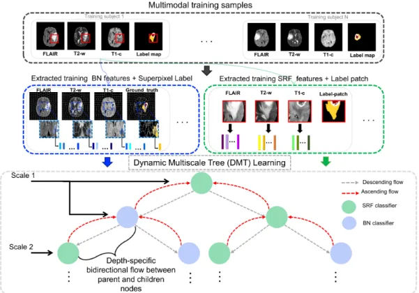
Figure 1: Proposed Dynamic Multi-scale Tree (DMT) learning architecture for multi-label classification (training stage). DMT embeds SRF and BN classifiers in a binary tree archi-tecture, where a depth-specific bidirectional flow occurs between parent and children nodes making the tree learning dynamic. During training, SRF learns a mapping between feature patches extracted from three MRI modalities and their corresponding label patches for each training subject; whereas BN classifier learns conditional probabilities from the superpixels of the oversegmented multimodal MR images and the label map.
segment the image at the superpixel level, thereby better capturing irregular
135
boundaries in the image.
2.2. Bayesian network
Bayesian networks are probabilistic graphical models based on directed acyclic graphs (DAGs) and Thomas Bayes’ theorem in probability theory giving a graphical representation of the probabilistic dependencies among a large number
140
of variables. BNs are increasingly applied for modeling complex systems and for the development of decision-making tools thanks to the following strengths: interdisciplinarity (the variables can be of different natures), graphical repre-sentation, ability to extend models by introducing new data observations, good management of uncertainty, noise or incomplete data. In particular, they are
145
characterized by adaptability to meet new needs. Thus, general BNs can be extended to solve address different challenges including cognitive modeling [21] evolution over time [22].
Technically, a BN is defined as an acyclic graph G(X, E) where nodes are associated to a set of random variables X = {X1, . . . , Xn} and links
repre-150
sent the dependencies between variables. For each node, we define conditional probabilitiesP =P(Xi|Pa(Xi)) relatively to its parent nodesPa(Xi) inG.
Various BN-based models have been proposed for image segmentation [17, 18, 19]. In our work, we adopt the BN architecture proposed in [19]. As a prepro-cessing step, we first generate the edge maps from the input MR image
modal-155
ities (Fig1). This edge map consists of a set of superpixelsSpi;i= 1, . . . , N (or
regional blobs) and edge segmentsEj;j= 1, . . . , L .
We define our BN as a four-layer network, where each node in the first layer stores a superpixel. The second layer is composed of nodes, each storing a single edge from the edge map. The two remaining layers store the extracted
super-160
pixel features and edge features, respectively. During the training stage, to set BN parameters, we define the prior probabilityP(Spi) ofSpi as a uniform
distri-bution and then learn the conditional probability representing the relationship between the superpixels’ features and their corresponding labels using a mixture
of Gaussians model. In addition, we empirically define the conditional
proba-165
bility modeling the relationships between each superpixel label and each edge state (i.e., true or false edge)P(Ej|Pa(Ej)) , wherePa(Ej) denotes the parent
superpixel nodes ofEj.
During the testing stage, we learn the BN structure through encoding the semantic relationships between superpixels and edge segments. Specifically, each
170
edge node has for parent nodes the two superpixel nodes that are separated by this edge. In other words, each superpixel provides contextual information to judge whether the edge is on the object boundary or not. If two superpixels have different labels, it is more likely that there is a true object boundary between them, i.e. Ej = 1, otherwise Ej = 0. The inference is conducted through
175
the BN using the MPE inference algorithm based on the factor graph called max-product algorithm [19].
Although automatic segmentation methods based on BN have shown great results in the state-of-the-art, they may perform poorly in segmenting low-contrast image regions and different regions with similar features [19]. To further
180
improve the segmentation accuracy of BN, we propose to include additional information through embedding BN classifier into our proposed DMT learning architecture.
3. Proposed Multi-scale Dynamic Tree Learning
In this section, we present the main steps in devising our Multi-scale
Dy-185
namic Tree segmentation framework, which aims to boost up the performance of classifiers nested in its nodes. Fig 1 illustrates the proposed binary tree architecture composed of classifier nodes, where each classifier ultimately com-municates the output of its learning (i.e., semantic context or probability seg-mentation maps) to its parent and children nodes. Therefore, the learning of the
190
tree is dynamic as it is based on ascending and descending feedbacks between each parent node and its children nodes. Specifically, each node output is fed to the children nodes as semantic context, in turn the children nodes transfer
their learning (i.e. probability maps) to their common parent node. Then, after merging these transferred probability maps from children nodes, the parent node
195
uses the merged maps as a contextual information to generate a new segmenta-tion result that will be subsequently communicated again to its children nodes. This gradually improves the learning of its classifier nodes at each depth level of the tree. In the following sections, we further detail the DMT architecture.
3.1. Dynamic Tree Learning
200
We define a binary tree T(Vt, Et), where Vt denotes the set of nodes in T
andEtrepresents the set of edges inT. Each nodeiinT represents a classifier
ci and each edge eij connecting two nodes iandj carries bidirectional
contex-tual information flow between the classifiersci andcj that are always inputting
the original image characteristics (i.e. the features for SRF, superpixel features
205
and input image edgemap for BN). Specifically, we define bidirectional feedbacks between two neighboring classifier nodesiandj, encoding two flows: a descend-ing flowFi→j that represents the transfer of the probability maps generated by
parent classifier nodeci to its child classifier nodecj as contextual information
and an ascending flow Fj→i that models the transfer of the probability maps
210
generated by a child nodecj back to its parent nodeci. This depth-wise
bidi-rectional learning transfer occurs locally along each edge between a parent node and its child node, thereby defining the dynamics of the tree. The DT traversal strategy is described in Algorithm 1.
In addition, as our Dynamic Tree (DT) grows exponentially, it integrates
215
various combinations of classifiers. Thus, each path of the tree implements a unique cascade of classifiers. To generate the final segmentation result we aggregate the segmentation maps produced at each leaf node in the binary tree by applying majority voting.
Inherent implicit and explicit transfer learning between nodes in
220
DT architecture. We note that the bidirectional flow between parent nodes and their corresponding children nodes defines a new traversing strategy of the tree nodes, that in addition to the dynamic learning aspect, encodes two
differ-Algorithm 1The Dynamic Multi-scale tree traversal algorithm Input:T:Binary Tree; Root: Root Node; data: classification data Output: classification results
queue Queue node N
Queue.Enqueue(Root)
whileN ot−Empty(Queue)do N←Queue.Dequeue
if N.P a=N U LLthen
/*Node without parent*/
N.P ostP rob←RunClassif ier(N.Classif ier, data)
/*RunClassifier(n,d,pb): Run the classification algorithm of node n considering the data d and the probability mappb and return the probability maps*/
else
N.P ostP rob←RunClassif ier(N.Classif ier, data, N.P a.P ostP rob) end if
if (N.lef t6=N U LL) and (N.right6=N U LL)then
/* Not a leaf node*/
P robL←RunClassif ier(N.Lef t.Classif ier, data, N.P a.P ostP rob) P robR←RunClassif ier(N.Right.Classif ier, data, N.P a.P ostP rob) F usionP rob←F usion(P robL, P robR)
/* fusion of the children probability maps*/
N.P ostP rob←RunClassif ier(N.Classif ier, data, F usionP rob) Queue.Enqueue(N.Lef t)
Queue.Enqueue(N.Right) end if
end while
apply majority voting strategy over the leaf nodes
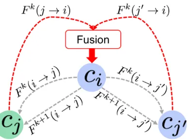
Figure 2: Implicit andexplicit learning transfer using ascending and descending flows. The dashed gray arrows denote the descending flows from the parent classifierCito his children
Ci and Cj0 while dashed red arrows denote the ascending flows derived from the children node to their parent, they are fused before being used by the parent node to generate a new segmentation map that will be be communicated to its two children classifier nodes.
ent types of learning transfer: explicit and implicit. Indeed, the ascending and descending flows between parent nodes and their children nodes through the
di-225
rect transfer of their generated probability maps is an explicit learning transfer. However, in our binary tree, when a parent nodeireceives the ascending flows (Fk(j→i) andFk(j0→i) from its left and right children nodesjandj0, they
are fused before being passed on, in a second round, as contextual information (Fk+1(i→j) andFk+1(i→j0)) to the children nodes (Fig. 2). The probability 230
maps fusion at the parent node level is performed through simple averaging. In particular, the parent node concatenates the fused probability map with the original input features to generate a new segmentation probability map result that will be communicated to its two children classifier nodes. Hence, the chil-dren nodes of the same parent node explicitly cooperate to improve their parent
learning, and implicitly cooperate to improve their own learning while using their parent node as a proxy.
SRF-BN Dynamic Tree. In this work, each classifier node is assigned a SRF or a BN model, previously described in Section 2, to define our Dynamic Tree architecture. The transferred information between classifiers through the
240
descending and ascending flows is used in addition to the testing image fea-tures as contextual information, while BN classifier uses this information as prior knowledge (i.e prior probability) to perform the multi-label segmentation task. The combination of SRF and BN classifiers is compelling for the following reasons. First, it enhances the performance of BN by taking the posterior
proba-245
bility generated by SRF as prior probability. This justifies our choice of the root node of our DT as a SRF. Second, it improves SRF performance around irreg-ular between-class boundaries since SRF benefits from BN structure learning, which is based on image over-segmentation that is guided by object boundaries. Third, as the SRF maps image information at the patch level, while BN models
250
knowledge at the superpixel level, their combination allows the aggregation of regular (i.e. patch) and irregular (i.e. superpixel) structures in the image for our target multi-label segmentation task.
3.2. Dynamic Multi-scale Tree (DMT) Learning
To further boost the performance of our multi-label segmentation
frame-255
work and enhance the segmentation accuracy, we introduce a multi-scale learn-ing strategy in our dynamic tree architecture by varylearn-ing the size of the input patches and superpixels used to grow the SRF and construct the BN classifier. Specifically, we use a different scale at each depth level so that, as we go deeper along the tree edges nearing its leaf nodes, we progressively decrease the size
260
of both patches and superpixels in the training and testing stages. In addi-tion to capturing coarse-to-fine details of the image anatomical structure, the application of the multi-scale strategy to the proposed DT allows to capture fine-to-coarse information. Indeed, DMT learning semantically divides the im-age into different patterns (e.g., different patches and superpixels at each depth
of the tree) in both intensity and label domains at different scales. However, thanks to the bidirectional dynamic flow, the scale defined at each depth influ-ences the performance of parent nodes (in previous level) and children nodes (in next level), which allows to simultaneously perform coarse-to-fine and fine-to-coarse information integration in the multi-label classification task. Moreover,
270
a depth-wise multi-scale feature representation adaptively encodes image fea-tures at different scales for each image pixel in the image element (superpixel or patch).
3.3. Statistical superpixel-based and patch-based feature extraction
To train each classifier node in the tree, we extract the following statistical
275
features at the superpixel level (for BN) and 2D patch level (for SRF): first order operators (mean, standard deviation, max, min, median, Sobel, gradient), higher order operators (Laplacian, difference of Gaussian, entropy, curvatures, kurtosis, skewness), texture features (Gabor filter), and spatial context features (symmetry, projection, neighborhoods) [23].
280
4. Results and Discussion
Dataset and parameters. We evaluate our proposed brain tumor seg-mentation framework using the Brain Tumor Image Segseg-mentation Challenge (BRATS 2015) dataset [24]. For each patient, we use three MRI modalities (FLAIR, T2-w, T1-c) along with the corresponding manually segmented glioma
285
lesions. They are rigidly co-registered and resampled to a common resolution to establish patch-to-patch correspondence across modalities. Then, we apply N4 filter for inhomogeneity correction, and use histogram linear transformation for intensity normalization.
For the baseline methods training we adopt the following parameters:(1)
290
Edgemap generation: we use the SLICE oversegmentation algorithm with a superpixel number fixed to 1000 and compactness fixed to 10 [? ]. To establish superpixel-to-superpixel correspondence across modalities for each subject, we
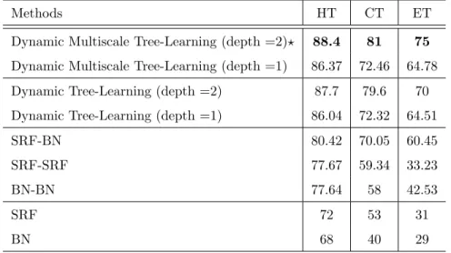
Methods HT CT ET Dynamic Multiscale Tree-Learning (depth =2)? 88.4 81 75 Dynamic Multiscale Tree-Learning (depth =1) 86.37 72.46 64.78 Dynamic Tree-Learning (depth =2) 87.7 79.6 70 Dynamic Tree-Learning (depth =1) 86.04 72.32 64.51
SRF-BN 80.42 70.05 60.45
SRF-SRF 77.67 59.34 33.23
BN-BN 77.64 58 42.53
SRF 72 53 31
BN 68 40 29
Table 1: Segmentation Dice score of the proposed framework and comparison methods av-eraged across BRATS 2015 patients. (HT: whole Tumor; CT: Core Tumor; ET: Enhanced Tumor; depth of the tree;?indicates outperformed methods withp−value≺0.05).
first oversegment the FLAIR MRI, then we apply the generated edgemap (i.e., superpixel partition) to the corresponding T1-c and T2-w MR images. (2) SRF
295
training: we grow 15 trees using intensity feature patches of size 10x10 and label patches of size 7x7. (3) BN construction: the BN model is built using the generated edgemap as detailed in Section 2; the conditional probabilities modeling the relationships between the superpixel labeling and the edge state are defined as follows: P(Ej = 1|Pa(Ej)) = 0.8 if the parent region nodes have
300
different labels, andP(Ej = 1|pa(Ej)) = 0.2 otherwise.
We used nested cross-validation to select the tree depth. If the performance becomes negligible from one depth level to the next one, we don’t further deepen the tree (stopping criterion). In our experiments, the training time for our DMT (with 3 levels, no use of GPU) is only about 5 hours for each traversal path
305
(total= 5×4 = 20h).
Evaluation and comparison methods. For comparison, as baseline methods we use: (1) SRF: the Random Forest version that exploits structural in-formation described in Section 2, (2) BN: the classification algorithm described
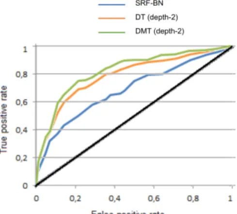
Figure 3: The ROC curves of three methods: SRF-BN, DT(depth=2), and DMT (depth=2).
in Section 2 where the prior probability of superpixels is set as a uniform
distri-310
bution, (3) SRF-SRF denotes the auto-context Structured Random Forest, (4) BN-BN denotes the auto-context Bayesian Network, where the first BN prior probability is set as a uniform distribution while the second classifier use the posterior probability of its previous as prior probability. Of note, by conven-tional auto-context classifier, we mean a uni-direcconven-tional contextual flow from
315
one classifier to the next one. The segmentation frameworks were trained using leave-one-patient cross-validation experiments. For evaluation, we use the Dice score between the ground truth region areaAgtand the segmented region area
Asas follows D= (AgtTAs)/2(Agt+As).
Next, we investigate the influence of the tree depth as well as the multi-scale
320
tree learning strategy on the performance of the proposed architecture.
Varying tree architectures. In this experiment, we evaluate two differ-ent tree architectures to examine the impact of the tree depth on the frame-work performance. Table. 1 shows the segmentation results for 2-level tree (i.e. depth=2) and 1-level tree (i.e. depth=1) for tumor lesion multi-label
segmen-325
tation with and without multiscale variant. We did not explore larger depths (d > 2), since as the binary tree grows exponentially, its computational time
dramatically increases and becomes demanding in terms of resources (especially memory). Furthermore, the improvement in its performance became negligible. Multi-scale tree architecture. To examine the influence of the multiscale
330
DT learning strategy, we compare the conventional DT architecture (at a fixed-scale) to DMT architecture. For the fixed-scale architecture, all tree nodes nest either an SRF classifier trained using intensity feature patches of size 10×10 and label patches of size 7×7 or a BN classifier constructed using an edgemap of 1000 superpixels generated with a compactness of 10. In the multiscale architecture,
335
we keep the same parameters of the fixed-scale architecture at the first level of the tree while the classifiers of the second level are trained with different parameters. Specifically, we use smaller intensity patches (of size 8×8) and label patches (of size 5×5) for the SRF training, and a smaller number of superpixels for BN construction (1200 superpixels).
340
Clearly, the quantitative results show the outperformance (improvement of 7%) of both proposed DT and DMT architectures in comparison with several baseline methods for multi-label tumor lesion segmentation with statistical sig-nificance (p ≤ 0.05) . This indicates that a deeper combination of different learning models helps increase the segmentation accuracy. When comparing
345
the results of the SRF and BN we found that SRF outperforms BN in segment-ing the three classes: wHole Tumor (HT), Core Tumor (CT) and Enhancsegment-ing Tumor (ET) (Table. 1 and Fig. 3). This is due to the fact that BN have diffi-culties in segmenting low-contrast images and identifying different superpixels having similar characteristics, especially with the lack of any prior knowledge
350
on the anatomical structure of the testing image. Although BN has a low Dice score compared to SRF, in Fig. 4 we can note that it has better performance in detecting the boundaries between different classes. This shows the impact of the irregular structure of superpixels used during BN training and testing, which gives BN the ability to be more accurate in detecting object boundaries
355
compared to SRF that considers regular image patches. Notably, BN struc-ture is individualized during the testing stage for each testing subject since it is based on the testing image oversegmentation map. Thus, SRF and BN classifiers
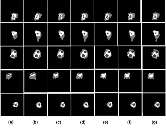
Figure 4: Qualitative segmentation results for all the baseline methods applied on 5 subjects: (a) the BN segmentation result; (b) the SRF segmentation result, (c) the auto-context BN; (d) the auto-context SRF; (e) SRF+BN segmentation result; (f) DMT segmentation results (depth=2); (g) the ground truth
are complementary. First, they perform segmentation at regular and irregular structures of the image. Second, one (SRF) learns image knowledge during the
360
training stage, while the other (BN) is structured using the input testing image during the testing stage through modeling the testing image structure. Further, the results of SRF-SRF and BN-BN models that implement the auto-context approach show an improvement of the segmentation results at both qualitative and quantitative levels when compared with baseline SRF and BN models. More
365
importantly, we note that BN-BN cascade outperforms SRF-SRF cascade when segmenting the Core Tumor and Enhancing Tumor (ET) lesions. This can be explained by the fine and irregular anatomical details of these image structures when compared to the whole tumor lesion. Since BN is trained using irregular superpixels, it produced more accurate segmentations for these classes (e.g.,
BN-370
BN:56.14 vs SRF-SRF: 37.12 for ET). Through further cascading both SRF and BN classifiers, we note that the heterogenoues SRF-BN cascade produced much better results compared to both autocontext SRF and autocontext BN for two main reasons. First SRF aids in defining BN prior based on the testing image structure , while BN enhances the performance of SRF at the boundaries level.
375
This further highlights the importance of integrating both regular and irregular image elements for training classifiers that capture different image structures. The outperformance of the proposed DMT architecture also lay ground for our assumption that embedding SRF and BN within our a unified dynamic architec-ture where they mutually benefit from their learning boosts up the multi-label
380
segmentation accuracy. In addition to the previously mentionned advantages of combining SRF and BN, it is important to note that the integration of variant cascades of SRF and BN endows our architecture with a an efficient learning ability, where it incorporates in a deep manner the knowledge of SRF based on modeling the dataset during the training step and the individualized learning
385
of BN based on the testing image during the testing step. Independently of the BN and SRF combination advantages, our DMT is a generic architecture based on optimized cascade classifiers through mutual dynamic learning trans-fer. Unlike several works that focuse on optimizing the learning of the classifiers
composing the cascade during the training stage [25, 26], our proposed DMT
390
architecture does not simply cascade classifiers, but it allows ensemble classifier learning in a dynamic and cooperative manner. The has exclusive characteris-tics. First, it is generic: each node can nest any elementary linear or non-linear deep classifiers (e.g., SVM, CNN).Second, it nicely encodes and integrates dif-ferent concepts that are well-founded in the state-of-the-art. Third, It allows
395
bidirectional learning transfer compared to other ensemble learning techniques. Compared to deep CNN based multi-label segmentation methods, it is of in-terest to know that our method is able to considerspatial consistency between neighboring superpixels and patches via the gradual autocontext feed between classifiers. Indeed, autocontext model is an iterative scheme that can
incorpo-400
rate the neighboring prediction information to compensate for the limitation of the independent pixel-wise (or patch-wise) estimation. In fact, the concept of cascading at multiple resolutions was proposed for face detection in [27] and shown to outperform single CNN. Since our DMT architecture clearly outper-formed simple cascades of classifiers, we anticipate that it will further improve
405
the performance of the ensemble learning of CNNs compared to multi-resolution CNN cascade. Furthermore, since our DMT is generic, it can embed any vari-ants of novel classifier cascades (e.g., cascades leveraging multi-task learning in [10]) while boosting the learning via the proposedbidirectional flow and implicit and explicit learning strategies. Our DMT can nest any classifier (e.g., deeply
410
supervised CNN [28]) and has the potential to boost the performance of simple as well as sophisticated ensemble classifiers that are only based on unidirectional flow of information between two consecutive classifiers. Hence, any classifica-tion method can be used as a base classifier in our architecture to enhance its performance.
415
Notably, our DMT architecture has a few limitations. First, it becomes more demanding in terms of computational and memory resources, as the tree grows exponentially (in the order ofO(2n)). The more nodes we add to the binary tree,
the slower the algorithm converges. Second, the patch and superpixel sizes in the multi-scale learning strategy can be further learned, instead of empirically fixing
them through inner cross-validation. Third, the bidirectional flow is currently restricted between neighboring parent and children nodes at a fixed tree depth. This can be extended to further nodes (e.g., root node), where the semantic context progressively diffuses from each node i along tree paths to far-away nodes. Fourth, our DMT was trained using simple feature extraction methods.
425
We anticipate that the performance of DMT learning will be further refined if one uses more advanced feature extraction and learning methods such as [29, 30, 31].
5. Conclusion
We proposed a Dynamic Multi-scale Tree (DMT) learning architecture that
430
both cascades and aggregates classifiers for multi-label medical image segmen-tation. Specifically, our DMT embeds classifiers within a binary tree archi-tecture, where each node nests a classifier and each edge encodes a learning transfer between the classifiers. A new tree traversal strategy is proposed where a depth-wise bidirectional feedbacks are performed along each edge between a
435
parent node and its child node. This allows explicit learning between parent and children nodes and implicit learning transfer between children of the same parent. Moreover, we train DMT using different scales for input patches and superpixels to capture a coarse-to-fine image details as well as a fine-to-coarse image structures through the depth-wise bidirectional flow. To sum up, our
440
DMT integrates compound and complementary aspects: deep learning, cooper-ative learning, dynamic learning, coarse-to-fine and fine-to-coarse learning. In our future work, we will devise a more comprehensive tree traversal strategy where the learning transfer starts from the root node, descending all the way down to the leaf nodes and then ascending all the way up to the root node.
445
We will also evaluate our DMT semantic segmentation architecture on different large datasets.
References
[1] M. Havaei, A. Davy, D. Warde-Farley, A. Biard, A. Courville, Y. Bengio, C. Pal, P.-M. Jodoin, H. Larochelle, Brain tumor segmentation with deep
450
neural networks, Medical image analysis 35 (2017) 18–31.
[2] S. Valverde, M. Cabezas, E. Roura, S. Gonz´alez-Vill`a, D. Pareto, J.-C. Vilanova, L. Rami´o-Torrent`a, `A. Rovira, A. Oliver, X. Llad´o, Improving automated multiple sclerosis lesion segmentation with a cascaded 3d con-volutional neural network approach, arXiv preprint arXiv:1702.04869.
455
[3] P. F. Christ, F. Ettlinger, F. Gr¨un, M. E. A. Elshaera, J. Lipkova, S. Schlecht, F. Ahmaddy, S. Tatavarty, M. Bickel, P. Bilic, et al., Auto-matic liver and tumor segmentation of ct and mri volumes using cascaded fully convolutional neural networks, arXiv preprint arXiv:1702.05970. [4] L. Folgoc, A. Nori, J. Alvarez-Valle, R. Lowe, A. Criminisi, Segmentation of
460
brain tumors via cascades of lifted decision forests, Proceedings of MICCAI-BRATS (2016) 35–39.
[5] X. Li, L. Wang, E. Sung, Multilabel svm active learning for image classifi-cation, Image Processing, 2004. ICIP’04. 2004 International Conference on 4 (2004) 2207–2210.
465
[6] Y. Wei, W. Xia, J. Huang, B. Ni, J. Dong, Y. Zhao, S. Yan, Cnn: Single-label to multi-Single-label, arXiv preprint arXiv:1406.5726.
[7] S. Lee, S. Purushwalkam, M. Cogswell, D. Crandall, D. Batra, Why m heads are better than one: Training a diverse ensemble of deep networks, arXiv preprint arXiv:1511.06314.
470
[8] Z. Tu, X. Bai, Auto-context and its application to high-level vision tasks and 3d brain image segmentation, IEEE Transactions on Pattern Analysis and Machine Intelligence 32 (10) (2010) 1744–1757.
[9] C. Qian, L. Wang, Y. Gao, A. Yousuf, X. Yang, A. Oto, D. Shen, In vivo mri based prostate cancer localization with random forests and auto-context
475
model, Computerized Medical Imaging and Graphics 52 (2016) 44–57. [10] J. Dai, K. He, J. Sun, Instance-aware semantic segmentation via
multi-task network cascades, Proceedings of the IEEE Conference on Computer Vision and Pattern Recognition (2016) 3150–3158.
[11] A. Rahman, S. Tasnim, Ensemble classifiers and their applications: A
re-480
view, arXiv preprint arXiv:1404.4088.
[12] H. Kim, J. Thiagarajan, J. Jayaraman, P.-T. Bremer, A randomized en-semble approach to industrial ct segmentation, Proceedings of the IEEE International Conference on Computer Vision (2015) 1707–1715.
[13] L. Breiman, Random forests, Machine learning 45 (1) (2001) 5–32.
485
[14] L. Yijing, G. Haixiang, L. Xiao, L. Yanan, L. Jinling, Adapted ensem-ble classification algorithm based on multiple classifier system and feature selection for classifying multi-class imbalanced data, Knowledge-Based Sys-tems 94 (2016) 88–104.
[15] P. Kontschieder, S. R. Bulo, H. Bischof, M. Pelillo, Structured class-labels
490
in random forests for semantic image labelling, Computer Vision (ICCV), 2011 IEEE International Conference on (2011) 2190–2197.
[16] J. Zhang, Y. Gao, S. H. Park, X. Zong, W. Lin, D. Shen, Segmentation of perivascular spaces using vascular features and structured random forest from 7t mr image, International Workshop on Machine Learning in Medical
495
Imaging (2016) 61–68.
[17] L. Zhang, Q. Ji, Integration of multiple contextual information for im-age segmentation using a bayesian network, Computer Vision and Pattern Recognition Workshops, 2008. CVPRW’08. IEEE Computer Society Con-ference on (2008) 1–6.
[18] C. Panagiotakis, I. Grinias, G. Tziritas, Natural image segmentation based on tree equipartition, bayesian flooding and region merging, IEEE Trans-actions on Image Processing 20 (8) (2011) 2276–2287.
[19] L. Zhang, Q. Ji, A bayesian network model for automatic and interactive image segmentation, IEEE Transactions on Image Processing 20 (9) (2011)
505
2582–2593.
[20] S. Yang, C. Yuan, B. Wu, W. Hu, F. Wang, Multi-feature max-margin hi-erarchical bayesian model for action recognition, Proceedings of the IEEE Conference on Computer Vision and Pattern Recognition (2015) 1610– 1618.
510
[21] A. Masoudi-Nejad, E. Wang, Cancer modeling and network biology: Accel-erating toward personalized medicine, Seminars in cancer biology 30 (2015) 1–3.
[22] P. Petousis, S. X. Han, D. Aberle, A. A. Bui, Prediction of lung can-cer incidence on the low-dose computed tomography arm of the national
515
lung screening trial: a dynamic bayesian network, Artificial intelligence in medicine 72 (2016) 42–55.
[23] M. Prastawa, E. Bullitt, S. Ho, G. Gerig, A brain tumor segmentation framework based on outlier detection, Medical image analysis 8 (3) (2004) 275–283.
520
[24] B. H. Menze, A. Jakab, S. Bauer, J. Kalpathy-Cramer, K. Farahani, J. Kirby, Y. Burren, N. Porz, J. Slotboom, R. Wiest, et al., The multimodal brain tumor image segmentation benchmark (BRATS), IEEE transactions on medical imaging 34 (10) (2015) 1993–2024.
[25] M. M. Dundar, J. Bi, Joint optimization of cascaded classifiers for
com-525
puter aided detection, Computer Vision and Pattern Recognition, 2007. CVPR’07. IEEE Conference on (2007) 1–8.
[26] A. Ellwaa, A. Hussein, E. AlNaggar, M. Zidan, M. Zaki, M. A. Ismail, N. M. Ghanem, Brain tumor segmantation using random forest trained on iter-atively selected patients, International Workshop on Brainlesion: Glioma,
530
Multiple Sclerosis, Stroke and Traumatic Brain Injuries (2016) 129–137. [27] H. Li, Z. Lin, X. Shen, J. Brandt, G. Hua, A convolutional neural
net-work cascade for face detection, Proceedings of the IEEE Conference on Computer Vision and Pattern Recognition (2015) 5325–5334.
[28] Q. Zhu, B. Du, B. Turkbey, P. L. Choyke, P. Yan, Deeply-supervised CNN
535
for prostate segmentation, Neural Networks (IJCNN), 2017 International Joint Conference on (2017) 178–184.
[29] W. Xiong, L. Zhang, B. Du, D. Tao, Combining local and global: Rich and robust feature pooling for visual recognition, Pattern Recognition 62 (2017) 225–235.
540
[30] B. Du, W. Xiong, J. Wu, L. Zhang, L. Zhang, D. Tao, Stacked convolutional denoising auto-encoders for feature representation, IEEE transactions on cybernetics 47 (4) (2017) 1017–1027.
[31] F. Zhang, B. Du, L. Zhang, L. Zhang, Hierarchical feature learning with dropout k-means for hyperspectral image classification, Neurocomputing
545