Learning Bayesian network structures with GOMEA

(1)

Kalia Orphanou

Centrum Wiskunde & Informatica Amsterdam, The Netherlands

[email protected]

Dirk Thierens

Universiteit Utrecht Utrecht, The Netherlands

[email protected]

Peter A. N. Bosman

Centrum Wiskunde & Informatica Amsterdam, The Netherlands

[email protected]

ABSTRACT

Bayesian networks (BNs) are probabilistic graphical models which are widely used for knowledge representation and decision making tasks, especially in the presence of uncertainty. Finding or learning the structure of BNs from data is an NP-hard problem. Evolutionary algorithms (EAs) have been extensively used to automate the learn-ing process. In this paper, we consider the use of the Gene-Pool Optimal Mixing Evolutionary Algorithm (GOMEA). GOMEA is a relatively new type of EA that belongs to the class of model-based EAs. The model used in GOMEA is aimed at modeling the depen-dency structure between problem variables, so as to improve the efficiency and effectiveness of variation. This paper shows that the excellent performance of GOMEA transfers from well-known academic benchmark problems to the specific case of learning BNs from data due to its model-building capacities and the potential to compute partial evaluations when learning BNs. On commonly-used datasets of varying size, we find that GOMEA outperforms standard algorithms such as Order-based search (OBS), as well as other EAs, such as Genetic Algorithms (GAs) and Estimation of Distribution algorithms (EDAs), even when efficient local search techniques are added.

CCS CONCEPTS

•Computing methodologies→Bayesian network models; • Genetic Algorithms; •Mathematics of Computing→ Bayesian networks;

KEYWORDS

Bayesian networks, evolutionary algorithms, structure learning ACM Reference Format:

Kalia Orphanou, Dirk Thierens, and Peter A. N. Bosman. 2018. Learning

Bayesian Network Structures with GOMEA. InGECCO ’18: Genetic and Evolutionary Computation Conference, July 15–19, 2018, Kyoto, Japan.ACM, New York, NY, USA, 8 pages. https://doi.org/10.1145/3205455.3205502

1 INTRODUCTION AND RELATED WORK

Bayesian networks (BNs) [12, 18] are probabilistic models that be-long to the class of graphical models. They were introduced as a

Permission to make digital or hard copies of all or part of this work for personal or classroom use is granted without fee provided that copies are not made or distributed for profit or commercial advantage and that copies bear this notice and the full citation on the first page. Copyrights for components of this work owned by others than ACM must be honored. Abstracting with credit is permitted. To copy otherwise, or republish, to post on servers or to redistribute to lists, requires prior specific permission and /or a fee. Request permissions from [email protected].

knowledge representation and inference approach under uncer-tainty through the use of probability theory and have been success-fully applied in diverse fields such as medical diagnosis, prognosis and image recognition.

A BN is a directed acyclic graph in which nodes represent random variables that denote an attribute, a feature or an hypothesis, such as a disease or a symptom. Arcs represent conditional probabilistic dependencies among variables. An arc fromAtoBindicates that the value taken by variableBconditionally depends on the value taken by variableA. Most of the time, BNs are interpreted to reflect cause-effect relationships. An arc then, fromAtoBindicates that Bis caused (or influenced) byA. To sample from a BN, the first step is to start from the nodes without parents, since for the rest of the nodes, a realization of the parents is needed, to index the conditional probability table for the particular node and then use that table to sample from, for that node. In case that there is no one variable without parents in the graph, the sampling process is not possible and the joint probability distribution would not be able to be defined. For that reason, a BN should always represent an acyclic graph.

The strength of these dependencies is quantified by local con-ditional probabilities. As an example, a BN applied in the medical domain could represent cause - effect relationships between a dis-ease, its causes and its symptoms. Given some symptoms and some of the disease causes (risk factors), the network can be used to compute the probability of the presence of a disease. More formally, a BN with a set of random variablesA=[A0, . . . ,A_m₋₁]consists of:

(1) A network structure that encodes the probabilistic condi-tional dependencies among the variables.

(2) A set of local conditional probability distributions

Pr(A_i|Pa(A_i))is associated with each node. Each probabil-ity distribution quantifies the effect of parents on the node. These are given as tables, in the case of discrete variables, which are called conditional probability tables (CPTs). For nodes that do not have any parents (i.e. the roots), their prior probability distribution is defined. Both prior and con-ditional probability tables are usually constructed from data with maximum likelihood estimation.

The network structure and the set of local probability distributions define the joint probability distribution forAas:

Pr(A0, . . . ,A_m₋1)= m−1

Ö

i=0

Pr(A_i|Pa(A_i))

Many algorithms have been proposed to address the optimiza-tion problem of learning the structure of a Bayesian network that

(2)

is a good representation of the data. The three most common ap-proaches are: a) constraint-based, b) score and search methods and c) hybrid methods.

Constraint-based methods use statistical hypothesis tests to de-tect a set of conditional independencies from the dataset. They use these dependencies to restrict the set of possible parents of each node, and build a BN based on these restrictions. They were the first developed algorithms for BN structure learning. The best known example of these methods is the PC algorithm [23].

Search and score methods, on the other hand, include a heuristic search procedure to search in the space of all possible networks, us-ing a scorus-ing metric to evaluate how well the network fits the data. There are several well-known proposed scoring metrics such as the Akaike’s Information Criterion (AIC) [1], the Bayesian Information Criterion (BIC) [22], the Minimum Description Length (MDL) [21] and the Bayesian Dirichlet equivalence (BDe) metric [22]. The gen-eral idea of the scoring methods is to compute the likelihood of the probability distribution that the BN encodes and to penalize this score in some form by the complexity of the network.

Previously studied score and search techniques involve heuristic search methods such as Simulated Annealing [11], Tabu search [3], Hill-Climbing (HC) [5] and K2 algorithm [4]. HC is the most well-known heuristic technique that uses a local search to find the solu-tion that maximizes the score. To prevent getting stuck in a local maximum, possible variations of HC include random-restart HC and its integration with tabu search.

Simulated annealing uses the Metropolis algorithm for optimiza-tion purposes. The search is terminated either based on a predefined termination criterion (e.g. maximum number of loops) or if there is not any improvement during the entire Metropolis loop. Tabu search searches iteratively through the neighborhood list of the current solution, and it stores the last visited solutions in the tabu list. In contrast to Simulated Annealing, Tabu search uses a memory (tabu list) to store a limited set of last visited solutions, which helps to prevent the method from being trapped in a local maximum. K2 takes as input a predefined node ordering and it searches through the set of solutions to find the network structure with the maximum score that should satisfy the predefined node ordering.

Recently, several hybrid methods have been proposed that com-bine both constraint and search and score strategies to improve the performance and the time complexity. The best known state-of-the-art hybrid methods include Sparse-Candidate (SC) algorithm [9], Max-Min Hill Climbing (MM-HC) [26] and the Ordering-based search [24].

Evolutionary algorithms (EAs) are another category of search and score methods that have been widely applied. The main advan-tage of the aforementioned algorithms is that EAs are less likely to get stuck in a local maximum (given a sufficiently large pop-ulation size and competent variation operators). They have been firstly proposed in [14] to discover the optimal node ordering us-ing crossover and mutation operators, that is passed on to the K2 algorithm. More work has followed for learning the best structure of the network using a heuristic search and a fitness function as a scoring method. A GA is further proposed in [13] to directly search for the optimal network structure in two scenarios: i) there is a node ordering assumption (parents before children) which reduces the dimension of the total set of possible structures and ii) there is

not any assumption and the algorithm should deal with a larger set of structures. As a follow up of this work, in [15], a local search operator is integrated to obtain better structures.

A skeleton-based approach for learning the structure of BNs was firstly proposed in [27, 28]. This approach consists of two steps: i) to build a BN skeleton from the data (an undirected graph) by using a constraint-based approach and ii) to run a score + search method, such as a GA, to search for the optimal structure, in the DAG space, but constrained by the skeleton.

In this work, we consider, for the first time, the use of a recently introduced EA, the Gene-pool Optimal Mixing Evolutionary Al-gorithm (GOMEA) [25], to search for optimal structures of BNs. GOMEA is a model-based EA that during optimization learns a linkage model that describes dependencies between problem vari-ables so that these are considered when generating new solutions, i.e. strongly dependent variables are always copied together when constructing a new offspring, so as to disrupt important building blocks as little as possible while mixing them.

GOMEA has been shown to outperform traditional genetic algo-rithms (GAs) and estimation-of-distribution algoalgo-rithms (EDAs) on many discrete single and multi-objective optimization problems, in terms of scalability and time complexity [25]. The main strengths of GOMEA, in contrast to classic GAs and EDAs, are its (often hier-archical) model-building capacities and the potential to use linkage models to perform efficient partial solutions during the variation process, if the problem at hand permits doing so.

The main aim of this paper is to evaluate the effectiveness and efficiency of GOMEA when learning the structure of BNs from data. To this end, we consider an integer-based representation of BN structures, and compare the performance of GOMEA on four benchmark network problems of various size with the performance of other EAs such as different variations of standard GAs, using various crossover operators, the ECGA [10], which is a well-known EDA, that also aims to detect and export problem structure, and other standard non EAs, which were reported in [6].

The remainder of this paper is organized as follows: In Sec-tion 2, a descripSec-tion of GOMEA is given. In SecSec-tion 3, a detailed description of the methodology used for learning BN using GAs is outlined, while in Section 4, the benchmark problems, the compared algorithms and the experimental results are presented. Finally, a discussion about the results is given in Section 6, while conclusions are presented in Section 7.

2 GENE-POOL OPTIMAL MIXING

EVOLUTIONARY ALGORITHM (GOMEA)

GOMEA [25] uses a general linkage model, namely the Family Of Subset (FOS)F. The FOS is a set of subsets of problem variables, having some degree of dependency, for which their values should be copied together when performing variation. A FOSFcan be written asF ={F0,F1, . . . ,F|F|−1}whereFi ⊂ {0,1, . . . ,l−1}, i∈ {0,1, . . . ,|F | −1}.

In the current study, we use the Linkage Tree Model (LT) struc-ture, which is the most often used FOS structure in literature on GOMEA [2]. In the LT model, linkage sets are arranged in a hi-erarchical tree structure that can be learned from a population of solutions by a hierarchical clustering procedure inO(nl2)time,

(3)

wherelis the number of problem variables andnis the population size.

An important aspect of GOMEA’s success is its main variation operator, called Gene-pool Optimal Mixing (GOM), that combines partial solutions to iteratively transform each solution in the popu-lation into exactly one offspring, thereby following the linkages as specified by the subsets. More precisely, an existing parent solution is duplicated. Then, each linkage set inFis traversed iteratively in a random order. For each set, a donor is randomly selected from the current population and its values for the variables indicated in the linkage set are copied to the parent solution. The partially altered solution is evaluated and its fitness is compared to the fitness of the parent solution. If the offspring solution has an equal or better fitness than the parent solution then the new generated solution is accepted, otherwise, it is reverted.

Note that, since GOM generates partially altered offspring solu-tions, the incorporation of the mechanism of partial evaluations for increasing the speed of the computation of the optimal solution is perfectly compatible in GOMEA. On the contrary, in GA or EDA, the offspring solutions are fully generated by mixing the values of the selected parents from the population, and the incorporation of the evaluation of partial solutions would be useless.

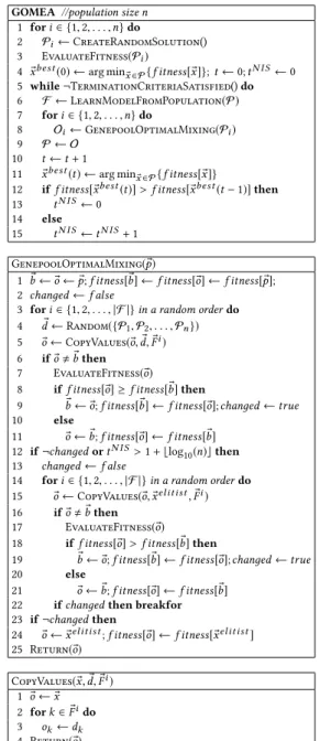
By its design, GOMEA could be seen to effectively integrate a form of linkage-based local search into variation, which makes its overall procedure closer to that of genetic local search, although with a dynamically learned neighborhood. In various problem do-mains, GOMEA has been shown to improve the performance com-pared to classic EAs. The current implementation of GOMEA is outlined in [16] and the pseudocode is displayed in Figure 1.

3 LEARNING BAYESIAN NETWORKS FROM

DATA WITH GAS

In this section, we describe how we represent BNs, evaluate fitness, perform local search and deal with infeasible solutions. These con-cepts can then straightforwardly be used to learn BNs from data with all types of GAs that we consider in this paper.

3.1 Representation

Each solution in the population is a fixed-length (l) string of inte-ger variables with three values. Each variable represents both the existence and the ordering of an arc between two variablesA_iand Aj. Thus, each parameter can take three possible values: i)0, if the arc betweenA_iandA_jis absent, ii)1, if there exists an oriented arc going fromA_i toA_j and iii)2, if there exists an oriented arc going fromA_j toA_i, wherei ∈ {0, ..,m−1}andj ∈ {i+1, ..,m−1}, wheremis the total number of variables.

A Bayesian network is a directed acyclic graph (DAG) and it is necessary to confirm that all the generated solutions represent acyclic graphs. Given that the existence of an arc between one variable to itself would not satisfy the constraint of acyclicity of the graph, the set of possible parents that a variable can have is equal tom−1, excluding itself. The total number of problem variablesl is therefore computed as:

l= m−1 Õ i=0 (m−i)= 1 2m (m−1)

GOMEA//population size n 1 fori∈ {1,2, . . . ,n}do

2 P_i←CreateRandomSolution() 3 EvaluateFitness(P_i)

4 x®best(0) ←arg min_®

x∈ P{f itness[®x]};t←0;tN I S←0 5 while¬TerminationCriteriaSatisfied()do 6 F ←LearnModelFromPopulation(P) 7 fori∈ {1,2, . . . ,n}do 8 O_i←GenepoolOptimalMixing(P_i) 9 P ← O 10 t←t+1 11 x®best(t) ←arg min_®

x∈ P{f itness[®x]}

12 iff itness[®xbest(t)]>f itness[ ®xbest(t−1)]then 13 tN I S←0

14 else

15 tN I S←tN I S+1 GenepoolOptimalMixing( ®p)

1 b®← ®o← ®p;f itness[®b] ←f itness[®o] ←f itness[ ®p]; 2 chanдed←f alse

3 fori∈ {1,2, . . . ,|F |}_{in a random order}do 4 d®←Random({P1,P2, . . . ,P_n}) 5 o®←CopyValues(®o,d®,F®i) 6 ifo®_,b®then

7 EvaluateFitness(®o) 8 iff itness[®o] ≥f itness[®b]then

9 b®← ®o;f itness[®b] ←f itness[®o];chanдed←true 10 else

11 o®← ®b;f itness[®o] ←f itness[®b] 12 if¬chanдedortN I S>1+⌊log

10(n)⌋then 13 chanдed←f alse

14 fori∈ {1,2, . . . ,|F |}in a random orderdo 15 o®←CopyValues(®o,x®el it ist,F®i) 16 _ifo®,b®then

17 EvaluateFitness(®o) 18 _iff itness[®o]>f itness[®b]_then

19 b®← ®o;f itness[®b] ←f itness[®o];chanдed←true 20 _else

21 o®← ®b;f itness[®o] ←f itness[®b] 22 _ifchanдed_{then breakfor} 23 if¬chanдedthen

24 o®← ®xel it ist;f itness[®o] ←f itness[®xel it ist] 25 Return(®o) CopyValues(®x,d®,F®i) 1 o®← ®x 2 fork∈ ®Fido 3 o_k←d_k 4 Return(®o)

Figure 1: Gene-pool Optimal Mixing Evolutionary Algo-rithm

The original implementation of GOMEA works on fixed-length strings of binary variables. The Linkage Tree is learned using a hierarchical clustering procedure where mutual information (MI) is employed as the basis of measuring the distance between two problem variables. Since the search space is still Cartesian, the extension of MI from computing the distance from binary to integer variables is straightforward [17].

3.2 Fitness Function

To evaluate the fitness of a BN, we use the uniform joint distribution likelihood-equivalence Bayesian Dirichlet (BDeu) score [4]. BDeu

(4)

is a scoring function that computes the marginal likelihood of data given a graph structure based on a prior Dirichlet distribution with parameter vectora

i jk. In the uniform distribution,a i jk =

1 qi

, where qiis the set of possible configurations of the parent set of a variable. BDeu is a decomposable score which can be written as a sum of functions that only depends on one variable and its parents. It is defined as follows: f(A,Pa(A))= m−1 Õ i=0 д(A_i,Pa(A_i)) where д(A_i,Pa(A_i))= qi−1 Õ j=0 loд Γ a i j Γ ai j+Ni j + ri−1 Õ k=0 loд© « Γai jk+Ni jk Γai jk ª ® ® ¬

whereΓ(v)is the Gamma function which forv ∈ _Nis given by Γ(v)=(v−1)!,a_{i j} =

ri−1

Í

k=0

ai jk,mis the total number of variables, ri represents the number of states ofA_i,N_{i jk} is the number of instances in the data where the variableA_i =k,k∈ {0, . . . ,r_i−1}, and the variables inPa(A_i)take theirj_{t h}configuration,

0≤j≤q_i −1, whileN_{i j}= ri−1 Í k=0 Ni jk.

3.3 Partial Evaluations

The first and foremost strength of GOMEA is its powerful way of learning and exploiting dependencies between problem vari-ables. An important additional benefit of GOMEA is that it becomes straightforward to incorporate a simple mechanism of performing partial evaluations that increases the speed of evaluating solutions. This is due to the fact that many subsets in the FOS have a limited size of problem variables, especially in the case of the Linkage Tree model. This leads to small changes to be evaluated, which in turn, leads to improvements in time requirements.

The particular way to achieve partial evaluations is based on the problem domain and the computation of fitness. It may not always be possible to do so. In the problem at hand, changing a few variables means that a few arcs may have been changed. Since the fitness function is the decomposable BDeu score, a sum of local BDeu scores over all BN nodes, the updated score for a BN is defined as follows:

LetC_i ∈ {0, . . . ,s−1}be the set of the nodes for which the parents have changed ands, the total number of nodes in this set, then: ∆f(A,Pa(A))= s−1 Õ i=0 д(C_i,Pa_new(C_i)) −д(C_i,Pa_old(C_i)) wherePa

old(Ci)is the set of the old parents of nodeC_i, andPa_new(C_i) is the set of the new parents of nodeC_i.

The BDeu score can be stored for each node so thatPa_old(C_i) does not have to be recomputed.

3.4 Local Search

The most common approach for searching an optimal network structure of a BN is by implementing a local search over the pos-sible set of networks using the operators of arc addition, deletion

and reversal. In this paper, we consider an integration of GAs and local search, as it is known that for many non-trivial optimization problems, adding local search is beneficial.

Local search is applied upon initialization and at the end of every generation, for every solution in the population. First, the solution is copied into a backup solution and then, the local search technique traverses iteratively through the set of all the problem variables in a random order. The current solution is partially altered by trying all possible values for each variable. In our case, the set of possible values of the problem variables are three: 0,1 or 2.

For each try, the partially-altered solution, after ensuring that is an acyclic graph, is evaluated and if there is an improvement in the fitness score, the new solution replaces the current one, otherwise it reverses to its backup solution.

3.5 Repair Operator

Building structures of a Bayesian network may result in illegal structures with GAs, i.e. cyclic directed graphs, due to mixing of different structure representations. In order to deal with this issue, a repair operator has been defined that ensures that graphs are acyclic. The operator is applied to every generated solution upon initialization and in every mixing step, prior to the evaluation of the fitness function.

Specifically, the repair operator uses Depth-First Search to detect cycles in the graph. It goes iteratively through all the nodes and keeps track of visited nodes using a recursive stack. In case that it reaches a node that is already stored in the recursion stack, then it detects a cycle in the graph. The last arc that completed the cycle is removed from the graph.

4 EXPERIMENTAL SETUP

4.1 Benchmark Datasets

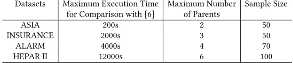
We used four well-known benchmark datasets of various sizes from the Bayesian Network Repository [8], i) a small BN, the ASIA network, withm=8 nodes, ii) a medium BN, the INSURANCE net-work, withm=27 nodes, iii) a medium BN, the ALARM network, withm=37 nodes and iv) a large BN, the HEPAR II network, with m=70 nodes.

For each network, 20 runs are repeated, where instances are randomly selected for the corresponding sample sizes given in Table 1. The fitness function used for all the experiments is the Bayesian score (BDeu) as described in Section 3.2. For final results, we consider the average BDeu score over 20 runs. We used the t-test to assess the statistical significance of our results.

4.2 Fully Controlled Comparisons

We first compare three GAs, the classic GA, an EDA and GOMEA. Doing so allows us to first isolate the impact of the different ways of performing variation for the problem of learning BNs from data. Choosing the most appropriate value for the parameter of the pop-ulation size is hard beforehand, especially in applications. The best population size depends on the specific EA and on the structure of the problem instance. We therefore use a population-sizing free scheme, that was previously proposed and tested for benchmark problems [16, 19]. In this scheme, multiple instances of an EA run in parallel and each instance has a different population size, where

(5)

Table 1: Parameters for the datasets

Datasets Maximum Execution Time Maximum Number Sample Size for Comparison with [6] of Parents

ASIA 200s 2 50

INSURANCE 2000s 3 50

ALARM 4000s 4 70

HEPAR II 12000s 6 100

larger populations have a slower generation cycle. This scheme can be integrated with any population-based optimization algorithm.

The GA that we consider here could be said to be a typical classic GA. It starts with a randomly generated population ofnsolutions. In every generation, an offspring populationOofnnew solutions is generated from the current populationPusing a recombination operator. This is repeatedntimes on two parent solutions that are randomly picked from the populationP, giving one offspring. In the current study, uniform crossover is used and offspring solutions are added to the population, resulting in aP+Opool of 2nsolutions in total, before tournament selection is performed with a tournament size of 4, to form the new parent population for the next generation. The EDA that we consider here is ECGA [10]. It starts with the initialization of a randomly generated population ofnsolutions. In every generation, a marginal product model (MPM) is learned from the population by merging sets of variables greedily, until the MDL metric can no longer be improved. The EDA does not use a recombination operator, like GA, but instead new solutions are generated by sampling the estimated probability distribution coded by the MPM. Similar as for the GA, tournament selection with a tournament size 4 is then performed to form the new population for the next generation.

4.3 Comparison with Literature

In addition, we compare our results with the recently published ones in [6]. The algorithms reported there are variants of the traditional GA using different crossover operators such as: Par-ent Set Crossover [6], Two-point Crossover [20], Half-Uniform Crossover [20] and Fitness-based Scanning Crossover [7].

In general, each substructure of BN consists of a node and the set of its parents. The Parent Set Crossover represents each of these substructures as a crossover block and an offspring is generated by recombining the parents of the nodes of two donors. The parents of every node of the offspring are the parents of the particular node in the randomly selected donor.

In Two-point Crossover, the middle parts from two randomly selected donors are combined to produce an offspring. Half-Uniform Crossover randomly swaps half of the differing values from two donors. The rest of the values are taken randomly from one of the two donors. Finally, the Fitness-based Scanning Crossover selects the value to extract from the donors, proportional to the fitness values of the donors.

We further compare with the non-evolutionary algorithms re-ported in [6]. These algorithms include Ordering-Based Search (OBS) [24], Sparse Candidate (SC) [9] and Max-Min Hill-Climbing (MMHC) [26]. OBS uses a greedy hill-climbing approach with a

tabu-list and random restarts to search over the possible set of node orderings, to find the one that maximizes the score of the structure. The computational cost of using a node ordering search space rather than the space of network structures is lower since the search space of node ordering is much smaller. Also, given the node ordering, the graphs are always acyclic and acyclicity checks are not needed. However, the main disadvantage of ordering-based search is that a large set of sufficient statistics has to be computed in advance.

SC is another hybrid method which uses a heuristic method to restrict the number of parents of each node and create a subset of the search space of the possible network structures. The mutual information measure is used to compute conditional dependencies between the nodes in the graph. Then, a hill-climbing heuristic method with tabu search is used to search over the network struc-tures for the one that maximizes the score. Finally, the MMHC is also a hybrid method that integrates a hill-climbing strategy with a constraint function. An example of the constraint function is the PC algorithm which restricts the possible parents of each node, based on their conditional dependencies. MMHC then uses the hill-climbing method with tabu-search on the restricted search space of network structures, to find the one that maximizes the score.

All the algorithms compared here that are reported in [6] have been implemented in MATLAB using the Bayesian Network Tool-box - Structure Learning Package (BNT-SLP). The machine used for the experiments in [6] has i7-2.60 GHz CP U and 32 GB RAM.

5 RESULTS

5.1 Fully Controlled Comparisons

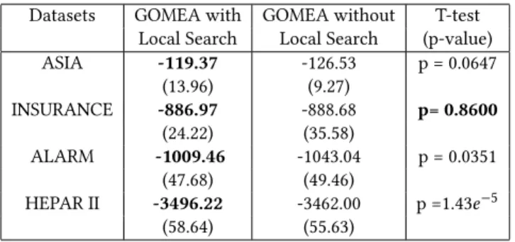
First, the t-test is used to assess statistical significance of the differ-ence of implementing GOMEA with local search and without local search, using as a termination criterion the maximum number of evaluations, setting toME=1,000,000. As displayed in Table 2, where the best performing results for each dataset are marked in bold, by including local search in the GOMEA implementation, there is an improvement in performance. All the results are statis-tically significantly different, except for the INSURANCE dataset results, where the incorporation of local search improves the results only slightly.

Second, the results of GOMEA with local search are compared with results of GA and ECGA, also with local search. Since GOMEA uses a partial evaluation mechanism, while GA and ECGA them-selves do not use any partial evaluations (i.e. only local search does this) for a fair comparison from a search perspective, we run the al-gorithms using as a termination criterion the maximum number of

(6)

Table 2: Average BDeu score of GOMEA with local search against GOMEA without local search, when using at most 1,000,000 evaluations. The standard deviation is displayed between parenthesis. The best BDeu scores and the statisti-cally insignificant different results are marked in bold.

Datasets GOMEA with GOMEA without T-test Local Search Local Search (p-value)

ASIA -119.37 -126.53 p = 0.0647 (13.96) (9.27) INSURANCE -886.97 -888.68 p= 0.8600 (24.22) (35.58) ALARM -1009.46 -1043.04 p = 0.0351 (47.68) (49.46) HEPAR II -3496.22 -3462.00 p =1.43e−5 (58.64) (55.63)

Table 3: Average BDeu score of GOMEA, GA and ECGA with local search and their standard deviation (displayed between parenthesis). The best BDeu scores are marked in bold.

Datasets GOMEA GA with ECGA

Uniform Crossover ASIA -119.37 -126.59 -126.62 (13.96) (9.28) (9.27) INSURANCE -886.97 -910.02 -926.89 (24.22) (38.61) (38.18 ) ALARM -1009.46 -1104.03 -1152.94 (47.68) (56.45) (51.69) HEPAR II -3496.22 -3536.49 -3541.87 (58.64) (59.98) (56.9)

evaluations, setting it toME=1,000,000. The comparison results (the average BDeu score over 20 runs) are displayed in Table 3 and the t-test results in Table 4. The best performing results for each dataset, as well as the results whose differences from the highest one are statistical insignificant(p>0.01), are marked in bold.

Third, the total execution time of GOMEA is computed against the GA and the ECGA with and without local search. In that case, we use a single run, since larger data samples give more accurate relative comparisons and for that large data samples, only one run is possible due to computation limitations. As a good representa-tive sample for a single run, we use the first 1,000 data instances (sample size) for all the networks, and as a termination criterion the maximum number of evaluations.

The results of the comparison, as displayed in Table 3, show that GOMEA outperforms both GAs. As also displayed in Table 4, the better performance of GOMEA is statistically significant.

In Table 5, the incorporation of local search improves the speed of GA and ECGA whilst without the incorporation of local search, as shown in Table 6, GOMEA is faster than both GAs. The reason for that is that GOMEA uses a model-based technique for the variation, where each parent is evolved iteratively with many small tests for improvements, whereas GA and ECGA use much more the local search technique during the variation. The technique that GOMEA

Table 4: P-value of the t-test of GOMEA comparing with the classic GA and ECGA. The results whose difference from GOMEA is statistically insignificant are marked in bold.

Datasets GA with ECGA

Uniform Crossover

ASIA p = 0.062 p = 0.062 INSURANCE p = 0.0307 p = 4.02e−4

ALARM p = 1.49e−6 p =4.34e−11 HEPAR II p = 0.0381 p = 0.0168

uses, is relatively more time consuming in between calls to the local search algorithm, but it does improve the results, since the obtained BDeu score of GOMEA is better than GA and ECGA for all the datasets.

The use of local search in the three GAs improves the speed of the algorithms when applying to a large dataset (e.g. HEPAR, 70 nodes), which is shown in Table 5, where the total execution time needed for the HEPAR dataset is less than for the rest of the datasets, (except the small ASIA dataset), for the same number of evaluations. This is due to the large number of evaluations used by the local search based on the number of problem variables, (l=2415, in the case of HEPAR), which leads the algorithms to find the better solutions using fewer generations than for the medium-size networks.

5.2 Comparison with Literature

GOMEA with local search has also been compared with the varia-tions of simple GA and other non EAs outlined in [6]. For a reason-able comparison, we use as a termination criterion for GOMEA the maximum running time, on a similar machine, used in [6]. The com-parison results (the average BDeu score over 20 runs) are displayed in Table 7 and the t-test results in Table 8. The best performing results for each dataset, as well as the results whose differences from the highest one are statistical insignificant(p >0.01), are marked in bold.

As displayed in Table 7, GOMEA outperforms all the comparison algorithms. The only exception is that the performance of MMHC, applied to the ALARM dataset, is slightly better than GOMEA but according to Table 8, this difference is statistically insignificant.

6 DISCUSSION

The superior performance of GOMEA transfers to the search space of learning the structure of Bayesian networks that is a good repre-sentation of the data, providing further evidence of the added value of GOMEA to the field of GAs and neighboring fields, such as AI that seeks to extract knowledge from data. The comparison that we used in this study, focuses mostly on the innate ability of GOMEA to search in the space of BN structures as a result of its variation operator, GOM, and how this compares to other GAs with other variation operators.

Compared to recently published results, GOMEA is superior when used to learn BNs for the benchmark problems, however, the obtained optimal solution represented by the best fitness score is not necessarily the best explanation of the causality dependencies in real-world case. For applying GOMEA, in real-world applications, a different fitness score or even added objectives should be taken into

(7)

Table 5: Total execution time (in s) for a single run (sample size = 1,000), with Local Search and the BDeu score between parenthesis, when using at most 1,000,000 evaluations. The best BDeu scores are marked in bold.

With Local Search

Uniform Crossover ASIA 179.181 104.750 98.586 (-1,929) (-2,230) (-2,230) INSURANCE 928.715 602.766 574.614 (-14,221) (-14,404) (-14,797) ALARM 1,440.011 775.513 446.623 (-11,860) (-13,280) (-12,885) HEPAR II 764.883 382.986 384.569 (-33,108) (-33,281) (-33,489)

Table 6: Total execution time (in s) for a single run (sample size = 1,000), without Local Search and the BDeu score between parenthesis. The best BDeu scores are marked in bold.

Without Local Search

Uniform Crossover ASIA 272.375 496.947 614.198 (-2,230) (-2,230) (-2,239) INSURANCE 4,092.844 10,946.564 13,744.575 (-14,166) (-14,191) (-15,336) ALARM 6,981.235 18,934.130 27,822.521 (-12,551) (-12,650 ) (-18,600) HEPAR II 14,564.191 33,245.270 100,800,000 (-33,157) (-33,304) (-33,578)

Table 7: Average BDeu score and the standard deviation (displayed between parenthesis) of GOMEA with local search and the results of the algorithms reported in [6], when using the maximum execution time as in Table 1. The best BDeu scores are marked in bold.

Datasets GOMEA GA with GA with GA with GA with SC OBS MMHC

Parent Set Two-Point Half-Uniform Fitness-based Crossover Crossover Crossover Scanning

ASIA -114.64 -129.29 -129.04 -129.21 -129.06 -129.33 -130.5 -129.34 (13.05) (8.35) (8.72) (8.44) (8.44) (8.43) (8.08) (8.12) INSURANCE -881.31 -1036.7 1069.9 -1036.9 1032.0 -1045.4 -1101.4 -1003.1 (23.24) (38.4) (38.2) (47.1) (42.8) (31.7) (52.8) (33.9) ALARM -988.44 -1020.8 -1028.5 -1023.4 -1022.2 -1016.4 -1078.1 -969.9 (44.25) (49.8) (47.3) (50.5) (50.1) (58.0) (55.4) (46.731) HEPAR II -3400.59 -3556.9 -3552.4 -3552.9 -3552.9 -3476.4 -3571.5 (58.53) (51.3) (51.4) (51.5) (51.5) (55.6) (53.3)

consideration. Especially if these objectives remain decomposable to an extent that partial evaluations are possible, the excellent and superior performance of GOMEA is expected to be retained. Moreover, as it stands, GOMEA is not necessarily yet optimally configured for the problem in this paper. In particular, specialized

local search techniques and/or constraint filters could be added to further boost its performance.

In general, the results show that GOMEA is a reliable and fast EA approach for searching for optimal structures of BNs from data, through a set of all the possible DAGs. This also raises the hypothe-sis that the incorporation of GOMEA as a search-and-score method

(8)

Table 8: P-value of the t-test of GOMEA comparing with the results in [6]. The results whose difference from GOMEA is statistically insignificant are marked in bold.

Datasets Parent Two- Half- Fitness- SC OBS MMHC

Set Point Uniform based

Crossover Crossover Crossover Scanning

ASIA p=1.81e−4 p=2.49e−4 p=1.98e−4 p=2.24e−4 p=1.79e−4 p=6.07e−5 p=1.64e−4 INSURANCE p=2.22e−16 p<0.0001 p=1.62e−13 p=2.20e−14 p<0.0001 p=1.11e−15 p=6.66e−15 ALARM p=0.04 p= 0.009 p=0.025 p=0.03 p=0.095 p=1.96e−6 p = 0.21 HEPAR II p=7.21e−11 p=1.55e−10 p=1.45e−10 p=1.45e−10 p=1.56e−4 p=9.81e−12

in the hybrid approaches, discussed in Section 1, could improve the performance and the computational time of the execution of those algorithms.

7 CONCLUSION

In this paper, we considered the use of a recently introduced EA, GOMEA, for learning the structure of a BN, using an integer-based representation, BDeu score as fitness, and a repair operator to en-sure acyclic graphs. We compared the performance of GOMEA against recently published results, as well as with other variations of GAs, applied to four benchmark datasets of various sizes. GOMEA obtains better scores than the algorithms compared here for almost all the datasets and its superior performance is also statistically significant. The incorporation of local search improves the perfor-mance of GOMEA even more.

Considering the results of our experiments, we believe that GOMEA can be used to effectively and efficiently learn Bayesian networks from data, more so than using other types of GAs. We therefore suggest that GOMEA should be taken into consideration, as a novel score-and-search EA method, either as presented here or combined with other methods, for learning the structure of BNs from data.

REFERENCES

[1] Hirotugu Akaike. 1974. A New Look at the Statistical Model Identification.IEEE Trans. Automat. Control19, 6 (1974), 716–723.

[2] Peter A.N. Bosman and Dirk Thierens. 2013. More Concise and Robust Linkage Learning by Filtering and Combining Linkage Hierarchies. InProceedings of the 15th Annual Conference on Genetic and Evolutionary Computation (GECCO ’13). ACM, New York, NY, USA, 359–366.

[3] Remco Bouckaert. 1995.Bayesian Belief Networks: From Construction to Inference. Ph.D. Dissertation. University of Utrecht.

[4] Wray L. Buntine. 1991. Theory Refinement on Bayesian Networks. In Proceed-ings of the Seventh Conference on Uncertainty in Artificial Intelligence. Morgan Kaufmann Publishers Inc., San Francisco, CA, USA, 52–60.

[5] Wray L. Buntine. 1994. Operations for Learning with Graphical Models._CoRR abs/cs/9412102 (1994).

[6] Carlo Contaldi, Fatemeh Vafaee, and Peter C. Nelson. 2017. The Role of Crossover Operator in Bayesian Network Structure Learning Performance: A Comprehen-sive Comparative Study and New Insights. In_{Proceedings of the Genetic and} Evolutionary Computation Conference, GECCO 2017, Berlin, Germany, July 15-19, 2017. 769–776.

[7] A. E Eiben, P-E Raue, and Zs. Ruttkay. 1994.Genetic Algorithms with Multi-parent Recombination. InInternational Conference on Parallel Problem Solving from Nature. Springer, 78–87.

[8] G. Elidan. 2001. Bayesian Network Repository. http://www.cs.huji.ac.il/site/labs/ compbio/Repository Accessed: 2018-01-31.

[9] Nir Friedman, Iftach Nachman, and Dana Peér. 1999. Learning Bayesian Network Structure from Massive Datasets: The Sparse Candidate Algorithm. InProceedings of the Fifteenth Conference on Uncertainty in Artificial Intelligence (UAI’99). Morgan Kaufmann Publishers Inc., San Francisco, CA, USA, 206–215.

[10] Georges R. Harik, Fernando G. Lobo, and Kumara Sastry. 2006. Linkage Learning via Probabilistic Modeling in the Extended Compact Genetic Algorithm (ECGA). In_{Scalable Optimization via Probabilistic Modeling}. Springer, 39–61.

[11] David Heckerman, Dan Geiger, and David M. Chickering. 1995. Learning Bayesian Networks: The Combination of Knowledge and Statistical Data.Machine learning 20, 3 (1995), 197–243.

[12] Daphne Koller and Nir Friedman. 2009.Probabilistic Graphical Models: Principles and Techniques. MIT Press.

[13] Larrañaga, Mikel Poza, Yosu Yurramendi, Roberto H. Murga, and Cindy M. H. Kuijpers. 1996. Structure Learning of Bayesian Networks by Genetic Algorithms: A Performance Analysis of Control Parameters. IEEE Transaction on Pattern Analysis and Machine Intelligence18, 9 (1996), 912–926.

[14] Pedro Larrañaga, Cindy M. H. Kuijpers, Mikel Poza, and Roberto H. Murga. 1997. Decomposing Bayesian networks: Triangulation of the Moral Graph with Genetic Algorithms.Statistics and Computing7, 1 (1997), 19–34.

[15] Pedro Larrañaga, Roberto Murga, Mikel Poza, and Cindy Kuijpers. 1996. Structure Learning of Bayesian Networks by Hybrid Genetic Algorithms. (1996), 165–174. [16] Hoang N. Luong, Peter A.N. Bosman, and Han La Poutré. 2017. Exploiting

Link-age Information and Problem-Specific Knowledge in Evolutionary Distribution Network Expansion Planning._{Evolutionary Computation}(2017), 1–35. [17] Hoang N Luong, Marinus O.W. Grond, Peter A.N. Bosman, and Han La Poutré.

2013.Medium-voltage Distribution Network Expansion Planning with Gene-pool Optimal Mixing Evolutionary Algorithms. In_{International Conference on} Artificial Evolution. Springer, 93–105.

[18] Judea Pearl. 1988. _{Probabilistic Reasoning in Intelligent Systems: Networks of} Plausible Inference. Morgan Kaufmann.

[19] José C. Pereira and Fernando G. Lobo. 2015. A Java Implementation of Parameter-less Evolutionary Algorithms.CoRRabs/1506.08694 (2015).

[20] Stjepan Picek, Marin Golub, and Domagoj Jakobovic. 2011. Evaluation of Crossover Operator Performance in Genetic Algorithms with Binary Representa-tion. InInternational Conference on Intelligent Computing. Springer, 223–230. [21] J. Rissanen. 1978. Modeling by Shortest Data Description.Automatica14, 5 (Sept.

1978), 465–471.

[22] Gideon Schwarz. 1978. Estimating the Dimension of a Model. The Annals of Statistics6, 2 (1978), 461–464.

[23] Peter Spirtes and Clark Glymour. 1991. An Algorithm for Fast Recovery of Sparse Causal Graphs.Social Science Computer Review9, 1 (1991), 62–72.

[24] Marc Teyssier and Daphne Koller. 2012. Ordering-Based Search: A Simple and Effective Algorithm for Learning Bayesian Networks._CoRRabs/1207.1429 (2012). [25] Dirk Thierens and Peter A.N. Bosman. 2011. Optimal Mixing Evolutionary

Algo-rithms. In_{Proceedings of the 13th Annual Conference on Genetic and Evolutionary} Computation (GECCO ’11). ACM, New York, NY, USA, 617–624.

[26] Ioannis Tsamardinos, Laura E. Brown, and Constantin F. Aliferis. 2006. The Max-min Hill-Climbing Bayesian Network Structure Learning Algorithm._Machine Learning65, 1 (Oct. 2006), 31–78.

[27] Steven Van Dijk, Dirk Thierens, and Linda C Van Der Gaag. 2003. Building a GA from Design Principles for Learning Bayesian Networks. In_{Genetic and} Evolutionary Computation Conference. Springer, 886–897.

[28] Steven van Dijk, Linda C Van Der Gaag, and Dirk Thierens. 2003. A Skeleton-based Approach to Learning Bayesian Networks from Data. InEuropean Confer-ence on Principles of Data Mining and Knowledge Discovery. Springer, 132–143.

ACKNOWLEDGMENTS

This work was carried out during the tenure of an ERCIM ’Alain Bensousassan’ Fellowship Programme.