Risk-Based Resource Allocation for Distribution System Maintenance

(1)

Risk-Based Resource Allocation

for Distribution System Maintenance

Final Project Report

Power Systems Engineering Research Center A National Science Foundation

Industry/University Cooperative Research Center since 1996

(2)

Power Systems Engineering Research Center

Risk-Based Resource Allocation

for Distribution System Maintenance

Final Project Report

Project Team

Ward Jewell, Project Leader, Joseph Warner

Wichita State University

James McCalley, Yuan Li

Sree Rama Kumar Yeddanapudi

Iowa State University

PSERC Publication 06-26

(3)

Information about this Project

For information about this project contact: Ward Jewell

Professor

Wichita State University

Department of Electrical and Computer Engineering Wichita, Kansas 67260-0044 Phone: 316-978-6240 Fax: 316-978-5408 Email: [email protected] James D. McCalley Professor

Iowa State University

Department of Electrical and Computer Engineering

Ames, Iowa 50011 Phone: 515-294-4844 Fax: 515-294-4263 Email: [email protected]

Power Systems Engineering Research Center

This is a project report from the Power Systems Engineering Research Center (PSERC). PSERC is a multi-university center conducting research on challenges facing the electric power industry and educating the next generation of power engineers. More information about PSERC can be found at the Center’s website: http://www.pserc.org.

For additional information, contact:

Power Systems Engineering Research Center Arizona State University

577 Engineering Research Center Box 878606

Tempe, AZ 85287-8606 Phone: 480-965-1643 FAX: 480-965-0745

Notice Concerning Copyright Material

PSERC members are given permission to copy without fee all or part of this publication for internal use, if appropriate attribution is given to this document as the source material. This report is available for downloading from the PSERC website.

(4)

Acknowledgements

This is the final report for the Power Systems Engineering Research Center (PSERC) research project titled “Risk-Based Maintenance Resource Allocation for Distribution System Reliability Enhancement” (PSERC project T-24). We express our appreciation for the support provided by PSERC’s industrial members and by the National Science Foundation’s Industry/University Cooperative Research Center program.

We are particularly grateful to MidAmerican Energy, the National Rural Electric Cooperative Association, and the Minnesota Valley Cooperative Light and Power Association for supplying data used in some parts of this project.

(5)

Executive Summary

Distribution systems are maintenance-intensive so maintenance budgets are a substantial share of costs for distribution businesses. Maintenance budgets are high, in part, due to the size of the systems and the number of people that it takes to properly maintain the system to achieve the appropriate reliability level. Operations and maintenance (O&M) budgets can be reduced through improved efficiency. However, of concern is the effect of such budget reductions on a distribution business’ ability to keep its system operating at the desired reliability level. To meet customer needs for affordable and reliable service while complying with regulatory requirements, with limited budgets, it is necessary to find tools and techniques that, when coupled with a sound asset management policy, can be used to optimally maintain distribution systems. Such a policy also extends equipment life to avoid or defer costly capital investments resulting from poor equipment maintenance.

In this project, we have developed a comprehensive and cost-effective maintenance allocation and scheduling system, and have implemented it in software tools. These tools assist in answering three concerns commonly faced by an asset manager:

1. How to identify and justify the resources needed for managing the assets of the entire system.

2. How to allocate the available resources to different maintenance programs. 3. How to select a set of maintenance tasks to be performed within each

maintenance program.

Our system allocates resources and schedules maintenance tasks to optimize system reliability by maximizing risk-reduction achieved from those tasks. It uses information obtained from inspection and monitoring to determine the state of the system. Available maintenance tasks are identified, and the risk reduction provided by each is computed. The risk reduction for each task is based on the condition of the component being serviced, the task’s effect on improving the component’s condition of equipment, and the resulting improvement in reliability indices. The tasks are prioritized, subject to constraints on available resources, using an optimization technique combining integer programming, Lagrange relaxation, and dynamic programming. For this initial development work, the maintenance tasks incorporated so far are associated with wood poles, reclosers, and vegetation management of distribution line right of way. Actually, maintaining these particular assets represents a large percentage of maintenance budgets; furthermore, outages of these assets can significantly affect system reliability. This work can be adapted to most types of distribution equipment.

The essential elements of the maintenance allocation and scheduling system include: 1. Failure mode identification: Taxonomies are essential in identifying the effects of

maintenance tasks on failure rates. We determined the taxonomies of failure modes together with maintenance tasks that address those failure modes.

2. Failure rate estimation: Failure rate reductions provided by each maintenance task were used to optimize the allocation of maintenance resources. Methods were developed for estimating the probabilistic failure rate for wood poles and

(6)

reclosers using condition measurements obtained from either continuous monitoring or from periodic inspection and testing. These methods also estimate the reduction in failure rate by maintenance task for each component.

3. Risk reduction due to maintenance: Using information on failure rate and its reduction by maintenance task, risk reduction was estimated with a reliability assessment tool developed in this project.

4. Maintenance task selection and prioritization: Risk reduction estimates form a pool of candidate maintenance tasks, along with their resource requirements. The system selects and prioritizes maintenance tasks based on the risk reduction obtained. Constraints on the optimization include the maintenance budget and level of labor resources. An integer programming optimization technique was developed for the selection and prioritization of candidate maintenance tasks. A degradation-path model to estimate failure probability and probability reduction was developed. This model was applied to wood poles to predict individual pole failure probability based on condition measurements that represent degradation in the pole’s residual strength.

A condition assessment technique was developed for reclosers. A check sheet for evaluating a recloser’s condition, either in the field or in the shop, is provided. The condition score is then correlated with historical data to provide an estimate of the recloser’s failure rate. Maintenance changes the recloser’s condition and thus its failure rate. Similar techniques can be applied to other distribution system components.

Research-grade software from this research includes:

1. Reliability evaluation tool: A predictive reliability evaluation tool was developed in Excel. It is used to compute system reliability levels. This software tool also computes sensitivities of reliability metrics to maintenance tasks. When combined with estimates of failure rate reduction obtained from maintenance tasks, the tool computes the risk reduction associated with maintenance. The output of this tool is one input to an optimizer tool that selects and prioritizes maintenance tasks. 2. Optimizer tool: An optimizer processes the inputs of (1) candidate maintenance

tasks, (2) effect of each task on reliability (i.e., risk reduction), (3) financial and labor resources needed for each maintenance task, and (4) available resources. The program selects and prioritizes maintenance tasks for the budget cycle.

Follow-on work to this project is needed. The reliability and inspection models developed should be further expanded, verified, and then adapted to other distribution equipment. Specifically, the wood pole degradation path model should be validated for other components with complex failure processes, such as switches and transformers. Similarly, the inspection methods developed for reclosers should be applied to other components, and the resulting failure rate estimates should be verified.

The problem formulation should be further enhanced by considering scheduling issues involved in equipment maintenance. The result will provide a schedule of planned maintenance for a budget period.

The optimal resource allocation strategy sacrifices some accuracy to solve the large-scale problem. Further research involving other optimization techniques will help improve the accuracy of the solution.

(7)

List of Tables

Table 3.1: Recloser score sheet... 14

Table 3.2: Condition of typical failed recloser ... 20

Table 3.3: Score for recloser in average condition ... 20

Table 3.4: Score for recently maintained recloser ... 21

Table 3.5: Population predictions ... 31

Table 3.6: Estimate of failure rate... 31

Table 3.7: Estimate of maintenance effect... 32

Table 4.1: Protection response of circuit breaker ... 38

Table 4.2: Protection response of fuse... 38

Table 4.3: Protection response of recloser... 39

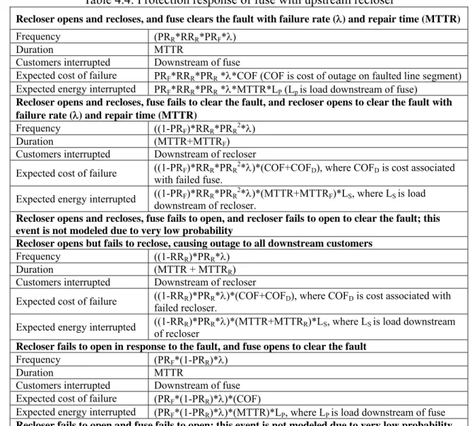
Table 4.4: Protection response of fuse with upstream recloser ... 40

Table 4.5: Protection response of sectionalizer with upstream recloser... 42

Table 4.6: Switching response for upstream isolation ... 43

Table 4.7: Switching response for downstream isolation ... 44

Table 4.8: Customer data ... 54

Table 4.9: Lengths of feeder section... 54

Table 4.10: Reliability indices for the ieee- reliability test system, bus 2 ... 54

Table 5.1. Risk reduction vs. budget... 56

Table 5.2. Decision variable code table ... 56

Table 6.1: Overall historical reliability indices for distribution system ... 63

Table 6.2: Historical indices—overhead, underground, and device failures... 63

Table 6.3: Historical indices—outages caused by miscellaneous failures ... 63

Table 6.4: Reliability parameter estimates for overhead lines and underground cables .. 64

Table 6.5: Reliability parameter estimates for protective and switching devices... 65

Table 6.6: Adjusted failure parameters for overhead and underground line segments .... 66

Table 6.7: Reliability indices using adjusted failure rates and repair times ... 66

Table 6.8: Reliability indices using adjusted failure rates and equivalent component... 66

Table 6.9: Failure modes and corresponding maintenance activities ... 68

(10)

List of Figures

Figure 1.1: Reliability benefit obtained from various resource-allocation levels... 1

Figure 1.2: Risk-based resource allocation for distribution systems. ... 5

Figure 3.1: Recloser score vs. failure rate... 19

Figure 3.2: Computing contingency probability reductions. ... 22

Figure 3.3: Flow chart of degradation model approach... 25

Figure 3.4: Number of poles at every age of the decayed population. ... 27

Figure 3.5: Decayed population Lspi(t) plot... 28

Figure 3.6 The average degradation level at every age. ... 28

Figure 3.7: Percentage of decayed pole at every age... 29

Figure 3.8: Hazard function of decayed poles. ... 30

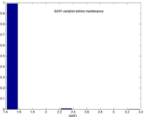
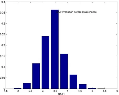
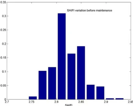
Figure 4.1: Variation in SAIFI before maintenance of wood pole. ... 48

Figure 4.2: Variation in SAIFI after maintenance of wood pole. ... 48

Figure 4.3: Variation in SAIFI before tree-trimming. ... 49

Figure 4.4: Variation in SAIFI after tree-trimming. ... 49

Figure 4.5: Variation in SAIFI before recloser maintenance... 51

Figure 4.6: Variation in SAIFI after recloser maintenance... 51

Figure 4.7: Variation in SAIDI before recloser maintenance. ... 52

Figure 4.8: Variation in SAIDI after recloser maintenance... 52

Figure 4.9: IEEE- reliability test system [36], bus 2... 53

Figure 5.1:Flowchart of ELPR-LRH optimization method. ... 58

Figure 5.2:Reliability benefit vs. budget... 60

Figure 5.3:Resource splitting curve for different categories. ... 60

Figure 6.1: Risk-based resource allocation implementation... 62

Figure 6.2: Risk reduction due to maintenance on reclosers. ... 69

Figure 6.3: Risk reduction obtained due to wood pole maintenance... 71

Figure 6.4: Risk reduction due to tree-trimming at a feeder level. ... 72

Figure 6.5: Budget vs. risk reduction... 73

Figure 6.6: Budget-splitting curve for different tasks... 73

Figure 6.7: Labor sensitivity... 74

Figure C.1. Input file of pole candidate tasks. ... 95

Figure C.2. Risk reduction versus budget table (ptable.m)... 96

(11)

1

Introduction

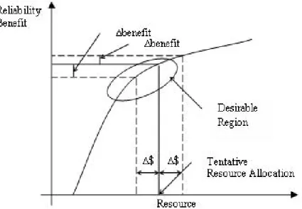
Both inspection and maintenance of equipment are a critical part of utility expenditures. It is important to ensure that every dollar spent helps improve the reliability and performance of the system. As illustrated in Figure 1.1, the ideal budgetary allocation results when the greatest benefit is obtained for every dollar spent. In this case, the benefit is reliability improvement indicated by relevant reliability indices.

From the asset manager’s point of view, a resource allocation within the indicated region in Figure 1.1 is desirable because it is the resource allocation for which the ratio of benefit to allocation is greatest. For larger resource allocations, this ratio falls off, and within the organization, the strength of the argument for obtaining such resource allocations diminishes.

This chapter describes, in detail, the challenge that asset managers face in maintaining their different distribution system assets. A brief review of common utility maintenance practices and their impact on reliability is discussed. A risk-based method of allocating maintenance resources is then proposed. Because of the limited resources available to this project, the methodology developed is limited to reclosers, vegetation, and wood poles. The methods developed for these can be adapted to other distribution equipment.

Figure 1.1: Reliability benefit obtained from various resource-allocation levels.

1.1

Asset Management Problem

Asset managers allocate resources among various maintenance activities. They are constrained by limited monetary and labor resources available for a broad array of maintenance activities. This presents a set of challenges to the asset manager that can be broadly classified into three categories.

The first is how to identify and justify the resources needed for asset management. Usually once a year, each asset manager must make a case for the financial and human resources required to manage equipment for which he/she is responsible. His/her

(12)

argument is best made in terms of the benefit obtained from the resources allocated. This establishes the total resources available to each asset manager.

Each manager must then decide how to allocate the available resources to different maintenance programs. 1 This secondary resource allocation distributes available resources from the first allocation to the different asset management programs. For this, the asset manager must understand how the total benefit from all programs changes as resources are shifted from one program to another.

The third problem is to select a set of maintenance projects2_{to be completed within}

each program, constrained by the secondary budgetary allocation. A solution to this problem allows the asset manager to compare the benefits of the different maintenance tasks available within a program and choose the best options depending on the resources available.

Apart from the above three issues, there may be a situation where certain parts of the system need to be maintained due to safety or regulatory requirements, regardless of the reliability benefit obtained. Such obligatory tasks also have to be addressed.

In order to find a comprehensive solution to each of the above problems, asset managers need tools to assess the benefit obtained from each maintenance task. Once that is determined, the corresponding cost and labor requirements can be used to judge the usefulness of the activity and prioritize accordingly.

1.2

State of the Art in Power System Maintenance

Before proposing a solution to the asset management problem presented in Section 1.1, a brief review of the state of the art in power system maintenance will be presented. Maintenance of a component reduces its failure rate and, thereby, the frequency and duration of interruptions experienced by customers. Utilities follow different procedures [1] or strategies to maintain different kinds of equipment. These maintenance practices can be broadly classified into two categories: corrective maintenance and preventive maintenance.

1.2.1 Corrective Maintenance

Also known as the run-to-failure strategy, corrective maintenance involves no maintenance of equipment until it fails. Once a component fails, it is replaced with a new or repaired component. This strategy can be disastrous in terms of reliability and can result in costly regulatory penalties. Most utilities have evolved from this method and use one or more of the following preventive maintenance strategies.

1.2.2 Time-Based Preventive Maintenance

Unlike corrective maintenance, preventive maintenance is done on equipment before a failure occurs, thus improving its condition and increasing the time before its next failure. In time-based preventive maintenance, a fixed time period is associated with each piece of equipment, after which it is replaced or maintained. This period is based on

1_{Program: A budgetary category within the asset management group. Programs are typically identified by a}

geographical region or type of equipment, e.g., tree-trimming, recloser maintenance, wood pole maintenance for a city or county, etc.

2_{Projects: A set of tasks within a particular program, e.g., tree-trimming for three feeders in a city, wood pole}

(13)

analysis of failure statistics and may use trial-and-error methods, expert judgment, or more analytical methods to estimate the optimal frequency of maintenance that is both economical and reliable at acceptable levels. The use of fixed-time period replacements, however, can lead to sub-optimal use of assets and unnecessary maintenance of equipment. Such strategies do not compensate for different conditions that identical components may experience on a system.

1.2.3 Condition-Based Preventive Maintenance

Condition-based preventive maintenance better allocates resources by using information regarding the current state of equipment to determine when and what kind of maintenance needs to be done. These methods require inspection and monitoring to estimate the piece of equipment’s condition and its remaining useful life before maintenance. Examples include dissolved gas tests for transformer oil, recloser operation counters, and visual inspection of feeders for vegetation growth. Condition information is used to predict the probability of component failure and the maintenance that is needed to prevent failure. Relative to time-based maintenance, condition-based methods typically extend the interval between successive maintenances and, therefore, reduce maintenance costs [2]. This method is restricted, however, to equipment whose cost of failure outweighs the inspection and monitoring costs incurred. Improved testing, monitoring, inspection, and data collection methods are needed to accurately predict the state of many power system components.

Condition-based maintenance uses information from equipment inspection and monitoring to estimate the condition of the equipment and schedule maintenance. The method does not, however, consider the effects of component failure or quantify the benefits of preventing failures. Decisions are made solely based on equipment condition, not its relative importance.

1.2.4 Reliability-Centered Maintenance (RCM)

Reliability-centered maintenance (RCM) is a preventive strategy that is being used increasingly by utilities. In this method, condition-based measurements are used to determine the various components that require maintenance. Maintenance projects are then ranked according to their effect on improving selected criteria. One or more reliability indices are usually chosen as the criterion, and maintenance projects are carried out to achieve desired target levels. While traditional maintenance programs, such as vegetation management, recloser maintenance, and maintenance of sectionalizing devices, are considered as discrete and unrelated programs, RCM provides a method to integrate a variety of programs and tasks with a single global objective of improving system performance [3].

1.2.5 Risk-Based Preventive Maintenance

Risk-based preventive maintenance methods further advance RCM [2]. Failure probabilities estimated by condition monitoring methods, along with the failure effects quantified by RCM methods, are used to determine the risk associated with failure of a particular piece of equipment. This risk is combined with the financial and human resource requirements to prioritize maintenance projects in order to maximize risk reduction.

(14)

For transmission systems, risk is defined as the time-dependent product of the probability of equipment failure and the consequence of its failure [2]. The consequence of failure is the quantified effect of equipment outage, such as overload of equipment, cascading failures, and low voltage. Risk-based maintenance is thus a form of RCM, with the following specific attributes when applied to transmission systems [2]:

a. Condition information is used to estimate equipment failure probability. b. Failure consequences are estimated and used in prioritizing maintenance tasks. c. Equipment failure probability and consequence at any particular time are

combined into a single metric called “risk.”

d. Equipment risk may be accumulated over a time interval (e.g., a year or several years) on an hour-by-hour basis to provide a cumulative risk associated with each piece of equipment.

e. The prioritization (and thus selection) of maintenance tasks is based on the amount of reduction in cumulative risk achieved by each task.

Selection and scheduling of maintenance tasks are performed at the same time (using optimization algorithms), since the amount of reduction in cumulative risk depends on the time when a maintenance task is implemented.

1.3

Risk-Based Allocation of Distribution System Maintenance

Resources

The objective of this work is to develop a similar risk-based strategy to allocate maintenance resources and prioritize maintenance projects for distribution system assets. The work will also provide a solution to the asset management problem discussed in Section 1.1. To do this, certain important differences between transmission and distribution need to be understood before extending the method to distribution systems.

First, unlike transmission systems, which are highly networked, most distribution systems are radial. Hence, the effects of an outage are localized, and the chance of cascading outages is very small. Furthermore, maintenance scheduled in one area can be assumed to be independent of the conditions in another region of the system. This is not the case in transmission systems, where maintenance of a component in one transmission region may restrict a task in another region due to stability constraints.

Second, distribution systems have a much larger number of components than transmission systems. The consequence of failure in most distribution components is thus lower than that in transmission components. This implies a large number of decision variables (candidate maintenance tasks) from which to choose and, hence, the need for optimization techniques that can suitably handle them.

Furthermore, the conditions in a distribution system are relatively constant or predictable compared to those in a transmission network, which can be highly dependent on such variables as network topology, loading, and equipment outages due to maintenance and environmental conditions.

This results in an important distinction in the nature of failure consequences. The consequence of failure of a specific transmission component is time varying and influences the short-term (hourly) as well as long-term (yearly) reliability indices. The failure consequence of a distribution component tends to be constant and thus can be well represented using the long-term or yearly indices.

(15)

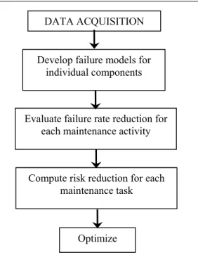
Figure 1.2 provides an outline of steps involved in the risk-based resource allocation strategy as it applies to distribution systems. Historical outage data and condition measurements are used to develop models that can predict equipment failure rates. The failure models are used to estimate how much each maintenance task will reduce a component’s failure rate. The effects of a failure are then related to changes in reliability indices. Failure rate reduction and the associated change in indices are used to compute the risk reduction associated with each maintenance task. Finally, tasks are selected and scheduled to maximize risk reduction subject to the resources available.

Figure 1.2: Risk-based resource allocation for distribution systems.

1.3.1 Definition of Risk

Every piece of equipment in the distribution system has a finite life, with failure probability that tends to increase with time. Maintenance improves the condition of equipment and thus reduces its likelihood of failure. In defining risk, the following effects of equipment failure will be considered:

a. Customer satisfaction, in terms of the expected number and duration of outages. b. Revenue lost by the utility due to energy not served.

c. Cost to replace or repair failed equipment.

d. Regulatory or contractual penalties paid by the utility due to missed reliability targets.

Repair and switching times for each component are assumed to be constant, and the distribution network configuration is considered fixed. This allows the reliability effects of each component to be expressed as linear contributions to the overall system indices [4]. These effects are expressed [4], [5] as follows.

DATA ACQUISITION Develop failure models for

individual components

Evaluate failure rate reduction for each maintenance activity

Compute risk reduction for each maintenance task

(16)

1.3.1.1 Effect on customer satisfaction

SAIFI, the system average interruption frequency index, is defined as

SAIFI = total number of customer interruptions / total number of customers served

for a given time period. For time period Δt, as a function of failure rate λk,l, for failure

mode l of component k, the contribution of failure mode l of component k to the system SAIFI is

(

)

N n t l k t SAIFI kl l k , ,. , | =λ Δ ⋅ (1.1)

with units of average number of interruptions per customer in time period Δt. The system SAIFI is the sum of these individual SAIFI contributions over all components k and failure modes l.

SAIDI, the system average interruption duration frequency index, is defined as SAIDI = sum of customer interruption durations / total number of customers served

for a given time period. The contribution of failure mode l of component k to the system SAIDI is

(

)

N d t l k t SAIDI l k n j j l k

∑

= ⋅ Δ = , 1 ,. , | λ (1.2)

with units of average hours of interruptions per customer in time Δt. The system SAIDI is the sum of the individual SAIDI contributions over all components k and failure modes l.

1.3.1.2 Revenue lost by the utility

(

)

∑

= ⋅ Δ = nkl j j j l k t Pd l k t ENS , 1 ,. , | λ (1.3)

1.3.1.3 Cost of equipment failure

(

t|k,l

)

_,. t Cost(k,l)

DevRisk =λ_k_l Δ ⋅ (1.4)

1.3.1.4 Regulatory penalties due to violation of regulatory limits

The effects expressed by equations (1.1) to (1.4) can be directly computed using standard analytical methods [6-9]. However, due to increased regulatory monitoring of reliability indices, it may be necessary for utilities to also estimate the risk of paying penalties that might arise from missed reliability targets. In such scenarios, it becomes necessary to estimate not only the average reliability indices for the system but also the variability in the indices [11] due to events that have low probability of occurrence with

(17)

substantially high penalties. The risk of penalties associated with each component may be defined as shown in equations (1.5) and (1.6).

t l k t SAIFI d l k t SAIFI f SAIFI PBR l k t PBRF F T Δ ⎪⎭ ⎪ ⎬ ⎫ ⎪⎩ ⎪ ⎨ ⎧ =

∫

∞ ( ). ( ( | , )) ( ( | , )) . ) , | ( (1.5) t l k t SAIDI d l k t SAIDI f SAIDI PBR l k t PBRD D T Δ ⎪⎭ ⎪ ⎬ ⎫ ⎪⎩ ⎪ ⎨ ⎧ =

∫

∞ ( ). ( ( | , )) ( ( | , )) . ) , | ( (1.6) where:

• λk,l is the failure rate of component ‘k’ due to a maintainable failure mode ‘l.’

• Δt is the time interval under consideration. • N is the total number of customers served.

• nk,l is the number of customers affected due to failure of component ‘k’ in mode

‘l.’

• dj is the duration of the interruption seen by the ‘j’th customer due to failure of

component ‘k’ in mode ‘l.’

• Pj is the load connected at point ‘j.’

• Cost (k,l) is the cost of failure for component ‘k’ in mode ‘l.’

• PBR(SAIFI) is a performance-based penalty for a SAIFI violation beyond threshold TF.

• PBR(SAIDI) is a performance based penalty for a SAIDI violation beyond threshold TD.

• f(SAIDI(t|k,l)) is a probability distribution of SAIDI obtained by non-sequential

Monte Carlo simulation for component ‘k’ in failure mode ‘l.’

• f(SAIFI(t|k,l)) is a probability distribution of SAIFI obtained by non-sequential

Monte Carlo simulation for component ‘k’ in failure mode ‘l.’

The time interval ‘Δt’ is assumed to be one year, so it can be removed from equations (1.1) to (1.6). As discussed in Section 1.3, the consequence of a component’s failure is assumed to be constant throughout the year. Unless the component is maintained, the component’s failure rate is also assumed to be constant throughout the year. This removes scheduling from the optimization problem, and leaves allocation of resources to programs and selection of maintenance tasks for the year.

Furthermore, the subscript ‘l,’ indicating the maintainable failure mode, can also be dropped without loss of generality, assuming that each of the equations (1.1) to (1.6) represents the consequences of equipment failure due to a single maintainable failure mode. Thus, the simplified expressions for the risk associated with each component can be correspondingly written, as shown in equations (1.7) to (1.12):

( )

N n k k SAIFI ₌ λ₍ _). k _(1.7)

( )

N d k k SAIDI k n j j

∑

= = 1 ). ( λ (1.8)

(18)

( )

∑

= = nk j j jd P k k ENS 1 ). ( λ (1.9)

( )

k (k).Cost(k) DevRisk =λ (1.10)

( )

= ∞

∫

(

( )

)

(

( )

)

F T k SAIFI d k SAIFI f SAIFI PBR k PBRF ( ). (1.11)

( )

=

∫

∞

(

( )

)

(

( )

)

D T k SAIDI d k SAIDI f SAIDI PBR k PBRD ( ). (1.12) The consequence of equipment failure may be expressed as the sum of the quantities defined by equations (1.7) to (1.12). This sum comprises the risk associated with a component’s failure. The risk associated with a component varies with its failure probability. If, during the time period under consideration, the failure rate of the component remains constant and is sufficiently low, the failure probability in equations (1.7) to (1.12) can be replaced with the failure rate of the component.

Maintenance reduces the failure rate of a component and thus the risk associated with its failure. The following expressions then can be used to define the effect of maintenance on a component:

( )

(

)

N n k N n k k k SAIFI k SAIFI k SAIFI k k A B A B − = − ⋅ = Δ ⋅ = Δ ( ) ( ) λ ( ) λ ( ) λ( ) (1.13)

( )

(

)

N d k N d k k k SAIDI k SAIDI k SAIDI k k n j j n j j A B A B

∑

= = ₌_Δ ⋅ − = − = Δ ₍ ₎ ₍ ₎ _λ ₍ ₎ _λ ₍ ₎ 1 _λ₍ _). 1 (1.14)

( ) (

)

∑

= = Δ = − = Δ k nk j j j n j j j A B k k P d k P d k ENS 1 1 ). ( . ) ( ) ( λ λ λ (1.15)

( ) (

k (k) (k)

)

.Cost(k) (k).Cost(k) DevRisk = λ_B −λ_A =Δλ Δ (1.16)

( )

=

∫

∞

(

( )

)

(

( )

)

− ∞

∫

(

( )

)

(

( )

)

Δ F F T A T

B k d SAIFI k PBR SAIFI f SAIFI k d SAIFI k SAIFI f SAIFI PBR k PBRF ( ). ( ). (1.17)

( )

=

∫

∞

(

( )

)

(

( )

)

−∞

∫

(

( )

)

(

( )

)

Δ D D T A T

B k d SAIDI k PBR SAIDI f SAIDI k d SAIDI k SAIDI f SAIDI PBR k PBRD ( ). ( ). (1.18) The subscripts ‘B’ and ‘A’ used in equations (1.13) to (1.18) correspond to the state of the component before and after maintenance, respectively. Thus, the overall risk reduction obtained from maintaining a component ‘k’ can be written as a linear combination of each of factors, as shown in equation (1.19).

(19)

4 4 4 4 4 8 4 4 4 4 4 7 6 4 4 8 4 4 7 6 48 47 6 4 4 4 4 4 8 4 4 4 4 4 7 6 penalties gulatory failure component of Cost revenue Lost on satisfacti Customer k PBRD k PBRF k DevRisk k ENS k SAIDI k SAIFI k Risk Re 6 5 4 3 2 1 ) ( . ) ( . ) ( . ) ( . ) ( . ) ( . ) ( Δ + Δ + Δ + Δ + Δ + Δ = Δ

α

(1.19)

The coefficients (αi) in equation (1.19) correspond to weights that an asset manager

assigns to the different factors based on their relative importance or confidence in their accuracy. By choosing the units appropriately for the coefficients (αi), the overall risk

reduction associated with a component’s failure can be represented by a single monetary value.

(20)

2

Maintenance Practices

This chapter reviews common maintenance practices for the following distribution components included in the methodology developed in this project: reclosers, vegetation, and wood poles.

2.1

Reclosers

Reclosers are very reliable devices that seldom fail. When failures do occur, however, they can lead to widespread outages and damage that significantly affect reliability indices and costs. Thus, many utilities use time-based preventive maintenance for reclosers, scheduling maintenance for all reclosers on the system every three to five years. Reducing the frequency of maintenance by using a risk-based methodology may significantly reduce recloser maintenance costs.

2.1.1 Failure Modes

Failure of reclosers can occur in four different modes: a. Failure to open.

b. Failure to close/reclose. c. False trip.

d. Failure to lockout.

Most failures are caused by improper settings. Causes of recloser failure fit within these four modes, and most can result in more than one type of failure mode.

Causes of recloser failure can be classified as follows:

a. Mechanical moving parts, including linkage, plunger, and contacts. b. Electrical insulation, including bushings, stringers, and oil.

c. Structural, which addresses the integrity of the tank. d. Improper setting or placement of a recloser.

e. Electronic, for electronic reclosers.

Preventive maintenance is performed to reduce the probability that these will occur.

2.1.2 Maintenance Practices

All but the very simplest recloser maintenance must be done in a shop; therefore, the recloser must be removed from service. When a recloser is removed, another recently serviced or new one is installed in its place. Since removal is costly, most utilities perform a standard maintenance procedure on each recloser that comes into the shop. The procedure returns the recloser to a serviced condition and reduces its failure rate.

During service of reclosers, oil is replaced or filtered. Mechanical parts, bushings, and stringers are inspected and replaced if they are damaged or excessively worn. Contacts are inspected for wear and replaced if needed. Insulation is tested to reduce the likelihood of internal or external recloser faults. Structural maintenance includes removing rust and repainting the tank can to a specified thickness of paint to reduce the effects of weather. When maintenance is complete, the recloser is tested to ensure that it is operating in accordance with its specified time curves. It is then returned to the warehouse for installation when needed.

(21)

2.2

Vegetation

Vegetation-related failures are a large contributor to distribution system interruptions. Utilities spend sizeable portions of their maintenance budgets controlling vegetation. Because of the high cost, utilities must assess the effectiveness of their vegetation maintenance programs.

2.2.1 Failure Modes

Tree growth into power distribution lines is less of a factor in distribution outages that it is in transmission. Most utility tree-trimming programs are effective in keeping growing vegetation away from distribution lines. Tree growth causes about 20 percent of sustained distribution outages, most of which are of short duration. Growth-related failures are maintainable and can be effectively controlled through regular tree-trimming [11].

Tree failures occur when branches or entire trees break and come into contact with the power-carrying conductors, resulting in short-circuited or downed conductors. Trees outside the actual right-of-way may fail and cause outages, which makes maintenance more difficult because utilities have limited authority outside of this area. Tree failure causes about 40 percent of all sustained distribution outages. These faults are often more severe and take longer to repair.

Some tree failures are preventable and thus maintainable, that is, if the tree shows external signs of decay or degradation. If identified, these failures can be corrected by providing structural support or removing dead or weak branches. Other tree failures, such as those caused by severe weather, may cause extensive damage to the distribution network. Such failures, which account for about 40 percent of all tree-related outages [12], are not maintainable.

2.2.2 Maintenance Actions

Corrective maintenance refers to repair activities done to restore the system after a fault. Crews are dispatched to locate the fault and remove the branch or tree from the circuit. They should also clear any overhang that may come in contact with the lines in the near future. Such maintenance is local and is aimed at restoring service to customers in the shortest possible time.

Preventive vegetation maintenance is done before a failure actually occurs and may include the following:

• Tree-trimming, which is the most common vegetation maintenance activity. Most utilities follow a three- to six-year cycle of trimming, whereby a specialized crew identifies vegetation overgrowth and trims to prescribed standards.

• Tree growth regulators. These are chemical agents used to slow vegetation growth rates and are typically used after trimming to slow regrowth.

• Tree removal. Utilities also remove trees that threaten the system, sometimes replacing them with shorter, slower-growing species.

• Spacer and tree cables. Insulated overhead conductors are used in areas requiring higher reliability and in regions where accessing the right-of-way is difficult. These cables allow vegetation to grow closer to the conductors and reduce the number of outages.

(22)

2.2.3 Inspection Methods

To identify areas where tree-related outages are likely to occur and to determine the proximity of trees to conductors, utilities have inspection programs to assess vegetation near their circuits. Vegetation is inspected visually, often midway between two tree-trimming cycles. Remote sensing and laser imagery, e.g., light detection and ranging (LiDAR), are also used.

Some utilities also have inspection activities that extend beyond the right-of-way. These hazard tree programs identify trees that are likely to fail and determine the maintenance needed, including reinforcement or replacement, to avoid failures.

2.2.4 Factors Influencing Failure Rates

A feeder’s vegetation-related failure rates are influenced by the following factors [13]:

a. Length of overhead lines.

b. Local density of vegetation, measured in number of trees per mile. c. Growth and regrowth rates of different species of vegetation. d. Climate, weather, and other environmental factors.

Since these factors may vary significantly among feeders, it is appropriate to model each individual feeder’s failure rate, if data is available.

2.2.5 Vegetation Condition and Modeling

Overhead feeders are repairable systems, and vegetation-related failures are a recurring process. When failures occur, repairs restore the system to a working state. Repair or maintenance decreases the failure rate of the system. However, the system tends to deteriorate as vegetation regrows and clearances decrease. This causes the number of tree-related outages to increase with time, thereby increasing the failure rate.

Vegetation management decreases, but does not totally eliminate, vegetation-related failures. The number of tree-related outages occurring in a unit of time may be used as a measure to estimate the state of the system. If this value is higher than a specified limit, the feeder may inspected to identify areas of maintenance. A low value indicates that no maintenance is required. This method can also be used to determine if the current trimming cycle is adequate.

Information that utilities maintain about tree-related outages is generally obtained from an outage management system. Such information may include the location, date, and time when the outage occurred, the time it took to repair the problem, the number of customers interrupted, and the time when service was restored. There is often, however, no information about the failure mode or maintenance performed.

Parametric failure rate models require information on each of these factors for individual feeders. Because such information is often not available, the use of non-parametric models may be necessary. Non-non-parametric models only require historical outage information and information about when the feeder was trimmed.

(23)

2.3

Wood Poles

Wood poles keep energized conductors and equipment away from the public and the ground, and maintain separation between conductors. Poles also serve as a support platform for equipment such as capacitors, regulators, and reclosers [14].

2.3.1 Decay of Wood Poles

Wood poles decay both internally and externally. Most decay is just below ground level, where moisture, temperature, air, and absence of direct sunlight are most favorable to the growth of fungi. This portion of the pole is also hidden from view and is close to its natural breaking point under strain. Thus, it is the most critical part of the pole and warrants special inspection and maintenance.

Wood pole failures usually occur as a result of physical stress such as wind, ice, or vehicle impact. The tendency of a pole to fail under such stress is related to the strength of the pole at ground level, where almost 90 percent of pole failures occur [15].

2.3.2 Detection and Measurement of Decay

Nondestructive evaluation methods estimate the effective area of the pole cross section at the ground line. Visual inspection is ineffective, since it will not reveal internal decay or decay below this point. Other approaches vary in accuracy and cost. These include acoustic [16] and resistance force [17], sometimes combined with measurements of humidity [18]. Another simple but cost-effective approach is to remove external decay and assess the internal decay by drilling into the pole. This project assumes measurements based on this approach.

2.3.3 Maintenance Practice

The primary maintenance on wood poles is ground line treatment [19], which can provide an economical extension of a pole’s physical life. Ground line treatment is recommended under the following conditions:

• Whenever a pole is inspected and the decay is not so far advanced that the pole must be replaced.

• Whenever a pole over five years old is reset.

• Whenever a used pole is installed as a replacement.

Ground line treatment consists of removing the external decay, followed by application of a preservative paste or grease. Then the treated section is wrapped, and the dirt around the pole is replaced.

A decayed pole can be stubbed, whereby the decayed section is simply cut off, if the remaining portion is long enough, strong enough, and in good enough condition. Stubbing costs one-third to one-half the cost of replacing a pole. If stubbing is not possible, the pole must be replaced when its residual strength is below applicable standards.

(24)

3

Failure Rate Estimation

This chapter presents models that estimate the failure rates of components, as well as the failure rate reduction achieved by preventive maintenance tasks.

3.1

Recloser

This section discusses the methodology for determining the condition of a recloser while in service. This condition data is then used to estimate the recloser’s failure rate.

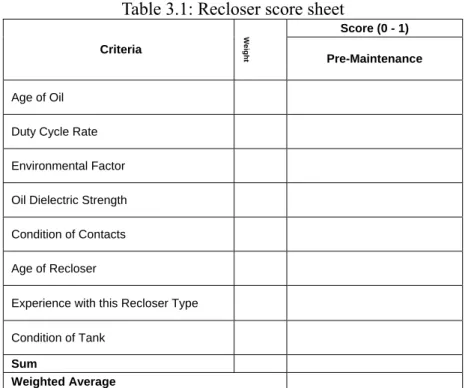
3.1.1 Condition Assessment

The methodology begins by assessing the condition of the recloser. A scoring sheet that itemizes relevant failure causes is shown in Table 3.1. Each of the criteria on the score sheet contributes to the reliability of a recloser, and most can be improved by preventive maintenance. Those that cannot be improved are still relevant in determining the recloser’s condition. These include the age of the recloser, which can only be improved by replacing the recloser, and the duty cycle rate and environmental factor, both of which are a function of placement on the distribution system rather than any maintenance performed.

For some reclosers, each of the criteria can be evaluated while the recloser is in service or from prior maintenance records. A large part of the cost of recloser maintenance is removing it from service, and removing a recloser from service to assess it, without performing maintenance, is never cost-effective. Components that can never be assessed in service are therefore omitted from Table 3.1.

Table 3.1: Recloser score sheet

Score (0 - 1) Criteria W e ight Pre-Maintenance Age of Oil

Duty Cycle Rate

Environmental Factor

Oil Dielectric Strength

Condition of Contacts

Age of Recloser

Experience with this Recloser Type

Condition of Tank

Sum

(25)

Scoring criteria are as follows:

• Age of Oil – The oil in a recloser is the most important dielectric in the unit, especially if the contacts are not in a vacuum. The oil helps extinguish arcs as contacts open and close, keeps arcs from occurring between other electrical conductors within the recloser, lubricates most of the moving parts, and is used to raise the trip piston after operation. The average expected life of oil is three years. Oil age thus provides a rough estimate of the oil’s dielectric strength without removing the recloser from service.

• Duty Cycle Rate – Duty cycle is a measure of the use a recloser has experienced since its last maintenance and is one of the most important criteria for determining when maintenance should be performed again. Duty cycle is a combination of the number of interruptions the recloser has performed, and either the percent of rated interrupting current or the circuit X/R value. NEMA has defined a standard duty cycle for distribution class reclosers [20]. Constant monitoring of every recloser’s duty cycle is impractical, so an alternate criterion, duty cycle rate, is defined. To calculate the duty cycle rate, the number of faults a recloser will see per year in a certain location is determined from the historical data used to calculate the utility’s SAIFI index. The value of system X/R at the recloser location is determined from system data. Then the NEMA standard duty cycle definitions give the number of operations per duty cycle for that location. Dividing the operations/cycle by the expected operations/ year gives the duty cycle in years/cycle for a recloser at that location. Duty cycle is then compared to expected oil life, whereby duty cycle rate equals the expected duty cycle divided by the expected oil life. This score is high for a high expected remaining duty cycle. If the score is greater than one, then the expected duty cycle is longer than the expected oil life, and the score is entered as one. This score is a function of recloser location on the system and not of the actual recloser condition.

• Environment Factor – This criterion is for reclosers in locations that require more frequent maintenance. It consists of a combination of recloser placement and environmental effects on the physical condition of the recloser. For example, a recloser bank protecting a feeder along a coastline will experience air with a much higher salt content than one located farther inland. The salt may cause the dielectric strength of the recloser oil to fall below standards much sooner than normal. This criterion addresses such conditions.

• Oil Dielectric Strength – This score is important if the utility’s recloser maintenance includes filtering the oil instead of replacing it. The score should be given as the difference between the post-maintenance oil dielectric strength, which is measured as part of maintenance, and the minimum allowable oil dielectric strength, divided by the difference between the new and minimum oil dielectric strengths.

• Condition of Contacts – This score is given as a percentage of remaining useful contact life.

• Age of Recloser – This is important because, as with all machines, reclosers become less reliable and fail with age. However, reclosers have proven to last for many years, and age has not been shown to be a reliable predictor of failure. Recloser age should still be monitored, though, as one indicator of condition.

(26)

• Experience with this Recloser Type – This criterion is used to differentiate among failure rates for different manufacturers or models, types, and sizes of reclosers. • Condition of Tank – If a tank has excessive damage, either from nature or

handling, the recloser may need maintenance before it is justified by the other factors.

3.1.1.1 Scoring

Recloser assessment begins with selecting the criteria for a particular recloser, as shown in Table 3.1. Different recloser types and models, for example, will use different criteria. Each recloser’s score will then be normalized by dividing the score by the maximum possible for the scored criteria. For example, evaluating contacts and oil dielectric strength for many reclosers requires removal from service. These criteria will not be included in the assessment or maximum possible score for those reclosers.

The score for each item is per unit of the remaining state of the recloser criterion. For example, if the contacts are 60 percent of their original size, their score would be 0.60. A recloser that has completed 75 percent of its recommended duty cycle would have a duty cycle score of 1.00 – 0.75 = 0.25, indicating the remaining 25 percent of its duty cycle. The resulting condition score, between 0 and 1, is denoted as xcs.

3.1.1.2 Weighting

The weight column in Table 3.1 represents the influence that a particular condition actually has on the failure rate of a recloser. Weights will be determined in practice by the combined opinion of manufacturers, utility engineers, and field personnel. Certain items are utility dependent, such as the environment factor inspection item.

3.1.2 Failure Rate Calculation

To relate a recloser’s condition score to its numerical failure rate, historical failure rate data from a number of systems were compiled for various power system components, including reclosers [21]. From this data, the best, worst, and average failure rates for each component were calculated. The resulting values for reclosers are as follows:

( )

0 =0.0025 λ (Best)

( )

1/2 =0.015 λ (Average)

( )

1 =0.060 λ (Worst)

If no historical data exists for the system to be modeled, then these values can be used. If, however, historical data is available for the system, then that data can, and should, be used to determine recloser failure-rate statistics for that system. Equation (3.1) [22] demonstrates how a system wide average recloser failure rate is calculated:

( ) (

Number of reclosers

) (

x Time period

)

failures recloser of number Total = 1/2 λ (3.1)

Ideally, the number of reclosers should be constant over the time period; a failure rate should be calculated for each such period, and then the failure rate for the entire period calculated from these values. The calculations are complicated by the inherent reliability and low failure rates of reclosers. The accuracy of the calculation thus depends on the

(27)

availability of such data and the time period over which it is available. Some utilities already have systems in place to collect data that can be used to track component reliability. Those that do not must use the best available data while gathering the needed information.

Also from the available data, the lowest and highest failure rates for reclosers on the system become the best, λ(0), and worst, λ(1), historical failure rates. If the calculated values are not judged to be accurate, then the published [21] values should be used.

From the historical failure rates, coefficients A, B, and C are calculated using equation (3.2) [21]:

[

]

( )

( ) ( )

A C A A B A − = ⎟ ⎠ ⎞ ⎜ ⎝ ⎛ + − = + − − = ) 0 ( ) 0 ( ) 2 / 1 ( ln 2 0 2 / 1 2 1 ) 0 ( ) 2 / 1 ( 2 λ λ λ λ λ λ λ λ (3.2)

These coefficients are recalculated periodically as data becomes available. Equation (3.3) then estimates the failure rate for an individual recloser, based on the coefficients and its condition [21]:

( )

x ₌ AeB*x ₊C

λ (3.3)

where λ(x) is the recloser’s failure rate, and x is a modified condition score that is calculated from the check sheet score xcs using equation (3.4):

x 1 xcs x1− x0 x1− − x0 xcs− x0 x1− (3.4) If xcs is used directly, then a recloser would need a score of xcs = 1 to be assigned the best

failure rate on the system, and a score of xcs = 0 to be assigned the worst. A recloser with

xcs = 0 would have completely failed every condition with a score of zero, which is not

practical. Instead, the best and worst scores on the system should relate to the best and worst historical failure rates. Thus, x1 is the worst recloser condition score recorded on

the system, and x0 is the best. The resulting value is subtracted from 1, because a high xcs

indicates a low failure rate, and a high x in equation (3.3) must represent a high failure rate.

Equation 3.4 will produce values that are negative when a recloser score xcs is greater

than the previous best score or greater than one when xcs is less that the previous worst

score. When this occurs, xcs replaces the previous best x1 or worst x0 historical score, as

shown in equations 3.5 and 3.6. Then x for the recloser is recalculated with the new values as follows:

If x < 0, then xcs is the updated x0 (3.5)

(28)

3.1.3 Effects of Maintenance

The maintenance tasks associated with each criterion on the score sheet are assumed to bring the score for that criterion to a predetermined value; this may be 1 or something less than 1. New post-maintenance coefficients, equation (3.2), and a new failure rate, equation (3.3), are calculated. Reliability indices for the system being simulated are then computed using the evaluation tool discussed in Chapter 4 and Appendix B. The calculated failure rates should then be calibrated so that the indices correlate with historical indices. A least-squares approach has been suggested for this [21], using the method of gradient descent.

3.1.4 Example

Six years of outage data were obtained from a utility and are used to illustrate the recloser assessment method. Out of 341 reclosers on the system, 23 recloser failures occurred during a 6.44-year period. Equation (3.1) produces an average failure rate λ(1/2) of 0.010473 44 . 6 * 341 23 (1/2) = = λ

The best and worst failure rates, λ(0) and λ(1), respectively, are then calculated. Each recloser on the system failed either zero times or one time during the six-year period. This gives failure rates of

λ(0) = 0 failure / 6.44 years = 0.00000 λ(1) = 1 failure / 6.44 years = 0.15528

These are too low and too high, respectively, to be practical; therefore, the following published failure rates [21] are used for the best and worst values: 

λ(0) = 0.0025

λ(1/2) = 0.010478021 λ(1) = 0.060

Next, the A, B, and C coefficients are calculated using equation (3.2) to be A = 0.0015321

B = 3.6514524 C = 0.0009679

The resulting equation (3.3) is

λ( )x := 0.0015321 ⋅e3.6514524 ⋅x + 0.0009679

(29)

0 0.1 0.2 0.3 0.4 0.5 0.6 0.7 0.8 0.9 1 0 0.01 0.02 0.03 0.04 0.05 0.06 λ( )x x

Figure 3.1: Recloser score vs. failure rate.

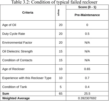
Best and worst historical scores for reclosers on the system were not available; therefore, the worst (x1) and best (x0) scores were assumed to be 0.31 and 0.95,

respectively. Table 3.2 then shows actual scores for a recloser that failed while in service. It was considerably past its expected duty cycle. Its condition score xcs was 0.392.

Equation (3.4) corrects this to

x 0.95 0.932− 0.95 0.31− x 0.872

which results in a failure rate, equation (3.3), of

λ(0.872) = 0.038

The low condition score, 0.392, as expected, produced a higher-than-average failure rate.

(30)

Table 3.2: Condition of typical failed recloser Score (0 - 1) Criteria W e ight Pre-Maintenance Age of Oil 20 0

Duty Cycle Rate 20 0.5

Environmental Factor 20 N/A

Oil Dielectric Strength 15 N/A

Condition of Contacts 15 N/A

Age of Recloser 10 0.65

Experience with this Recloser Type 10 0.7

Condition of Tank 5 0.4

Sum 65 25.5

Weighted Average 0.392307692

Next, a recloser in near-average condition was scored, as shown in Table 3.3. Table 3.3: Score for recloser in average condition

Score (0 - 1) Criteria W e ight Pre-Maintenance Age of Oil 20 0.33

Duty Cycle Rate 20 0.9

Sum 65 43.35

(31)

λ 0.95 0.667− 0.95 0.31−

⎛⎜

⎝

⎞⎟

⎠

= 0.00867

which is close to the system average failure rate of 0.01048.

Finally, Table 3.4 shows scores for a relatively new recloser that underwent scheduled maintenance about a year before it was scored. This is indicated by the age of the oil in the recloser. The recloser is not expected to complete a duty cycle before the oil is due to be changed again.

Table 3.4: Score for recently maintained recloser

Score (0 - 1) Criterion W e ight Pre-Maintenance Age of Oil 20 0.66

Duty Cycle Rate 20 1

Sum 65 55.95

The estimated failure rate for this recloser is

λ 0.95 .861−

0.95 0.31−

⎛⎜

⎝

⎞⎟

⎠

= 0.00351

which is close to 0.0025, the best failure rate previously found on the system.

A condition score, xcs, of 0.30, produces an equation (3.4) score, x, of 1.015. This

score of 0.30 replaces (equation (3.6)) the previous historical low score of 0.31, and the recloser is assigned the lowest historical failure rate on the system.

3.1.5 Summary

This methodology allows for quantifiable assessment of a recloser’s condition. The assessment is designed to be done in the field without removing the recloser from service. The assessment score is converted to an estimated failure rate, which is based on historical data.

(32)

The assessment criteria are directly related to maintenance tasks that may be performed on the recloser. Each maintenance task will increase the score for the associated criteria, resulting in a lower calculated failure rate. This method can be adapted to other power system components.

3.2

Vegetation

Another approach to computing failure probabilities is illustrated in Figure 3.2, based on a multi-state Markov probability model, where each of the J states is represented as a deterioration level. Boundary conditions separating J states of deterioration in component

k are defined in terms of the measurements ck(t), using the deterioration function g(ck(t)).

The deterioration function returns a deterioration level j identified by dj-1<g(ck(t))<dj,

where the last state j=J represents the failed state. State J need not represent the relatively rare catastrophic failure, for which very little data is typically available. Rather, state J

represents a set of measurement values for which engineering judgment indicates the component should be removed from service. The particular representation in Figure 3.2 shows J=4 deterioration levels, and deterioration level j can be reached only from deterioration level j-1. However, the model is flexible so that any number of deterioration levels can be represented, and if data indicates that transitions occur between non-consecutive states (e.g., state 1 to state 3), then the model can accommodate this easily. The transition from level 4 to level 1 stochastically represents the effects of maintenance, and if the decision problem is whether to maintain or not (a deterministic result of the problem), then we would set μ41=0. The steps to implementing this approach are

described as follows. λjk Deterioration Function g(c(T+1)) Historical Data c(t) t=1,…,T Statistical Processing μ41 λ23 λ12 λ34 Most Recent Observation c(T+1) Level 1 (new) Level 2 (minor) Level 3 (major) Level 4 (failed)

Figure 3.2: Computing contingency probability reductions.

a. Deterioration function: The deterioration function, denoted by g(ck), may be an

analytical expression, if one is available, or it may be a set of rules encoded as a program, likely consisting of a nested set of if-then statements that returns a scalar assessment value. For the model of Figure 3.2, the assessment value would be a deterioration level 1, 2, 3, or 4.

This represents a flexible and practical way of connecting our approach to the wealth of existing knowledge and experience contained in the industry relative to interpreting

(33)

condition monitoring measurements. Often, such rules depend not only on the measurements ck(t) but also on the rates of change in such measurements. These rules,

together with expertise provided by industry advisors, are used to develop the deterioration functions. For example, a comprehensive compilation of such rules for transformers [23] provides 62 different measurements for characterizing 23 transformer failure modes. Examples, and some of the failure modes they detect, include dissolved gas analysis results on main tank oil (indicating insulation deterioration, deterioration of cooling system, or oil pump failure) and load tap changer oil (indicating oil dielectric weakening), thermography testing (indicating magnetic circuit overheating or bushing overheating), ultrasonic testing (indicating oil pump failure), partial discharge testing (indicating magnetic circuit overheating), and winding and oil temperature measurements (indicating deterioration of the transformer cooling system).

Little has been published on correlating equipment deterioration with operating histories, a fact that stems from the difficulty in obtaining and merging operating and condition data in ways that properly characterize deterioration. Statistical modeling and analysis can be used to capture such trends, however. For vegetation, probabilistic vegetation failure rate models developed in [13, 24], are used to capture deterioration in this failure mode.

b. Transition intensities: Transition intensities between the various states of the model can be obtained from life histories of multiple units of the same manufacturer and model. In the case of Figure 3.2, λ12, λ23, and λ34 are needed. Consider a set of condition

measurements c(t)=[c1(t),c2(t),…,cK(t)] for K similar components taken over an extended

period of time t=0,1,…,T. For component i, the deterioration function is used to compute the deterioration level indicated by each measurement. This gives the time the component spent in deterioration level j. The mean of the durations for all components