Real-time crash prediction of urban highways using machine learning algorithms by
Mirza Ahammad Sharif
B.S., University of Asia Pacific, 2011 M.S., University of Wyoming, 2015
AN ABSTRACT OF A DISSERTATION
submitted in partial fulfillment of the requirements for the degree
DOCTOR OF PHILOSOPHY
Department of Civil Engineering Carl R. Ice College of Engineering
KANSAS STATE UNIVERSITY Manhattan, Kansas
Abstract
Motor vehicle crashes in the United States continue to be a serious safety concern for state highway agencies, with over 30,000 fatal crashes reported each year. The World Health Organization (WHO) reported in 2016 that vehicle crashes were the eighth leading cause of death globally. Crashes on roadways are rare and random events that occur due to the result of the complex relationship between the driver, vehicle, weather, and roadway. A significant breadth of research has been conducted to predict and understand why crashes occur through spatial and temporal analyses, understanding information about the driver and roadway, and identification of hazardous locations through geographic information system (GIS) applications. Also, previous research studies have investigated the effectiveness of safety devices designed to reduce the number and severity of crashes. Today, data-driven traffic safety studies are becoming an essential aspect of the planning, design, construction, and maintenance of the roadway network. This can only be done with the assistance of state highway agencies collecting and synthesizing historical crash data, roadway geometry data, and environmental data being collected every day at a resolution that will help researchers develop powerful crash prediction tools.
The objective of this research study was to predict vehicle crashes in real-time. This exploratory analysis compared three well-known machine learning methods, including logistic regression, random forest, support vector machine. Additionally, another methodology was developed using variables selected from random forest models that were inserted into the support vector machine model. The study review of the literature noted that this study’s selected methods were found to be more effective in terms of prediction power. A total of 475 crashes were identified from the selected urban highway network in Kansas City, Kansas. For each of the 475 identified crashes, six no-crash events were collected at the same location. This was necessary so that the
predictive models could distinguish a crash-prone traffic operational condition from regular traffic flow conditions. Multiple data sources were fused to create a database including traffic operational data from the KC Scout traffic management center, crash and roadway geometry data from the Kanas Department of Transportation; and weather data from NOAA. Data were downloaded from five separate roadway radar sensors close to the crash location. This enable understanding of the traffic flow along the roadway segment (upstream and downstream) during the crash. Additionally, operational data from each radar sensor were collected in five minutes intervals up to 30 minutes prior to a crash occurring.
Although six no-crash events were collected for each crash observation, the ratio of crash and no-crash were then reduced to 1:4 (four non-crash events), and 1:2 (two non-crash events) to investigate possible effects of class imbalance on crash prediction. Also, 60%, 70%, and 80% of the data were selected in training to develop each model. The remaining data were then used for model validation. The data used in training ratios were varied to identify possible effects of training data as it relates to prediction power. Additionally, a second database was developed in which variables were log-transformed to reduce possible skewness in the distribution.
Model results showed that the size of the dataset increased the overall accuracy of crash prediction. The dataset with a higher observation count could classify more data accurately. The highest accuracies in all three models were observed using the dataset of a 1:6 ratio (one crash event for six no-crash events). The datasets with1:2 ratio predicted 13% to 18% lower than the 1:6 ratio dataset. However, the sensitivity (true positive prediction) was observed highest for the dataset of a 1:2 ratio. It was found that reducing the response class imbalance; the sensitivity
sensitivity was found to increase with an increase in training data. The logistic regression model found an average of 30.79% (with a standard deviation of 5.02) accurately. The random forest models predicted an average of 13.36% (with a standard deviation of 9.50) accurately. The support vector machine models predicted an average of 29.35% (with a standard deviation of 7.34) accurately. The hybrid approach of random forest and support vector machine models predicted an average of 29.86% (with a standard deviation of 7.33) accurately.
The significant variables found from this study included the variation in speed between the posted speed limit and average roadway traffic speed around the crash location. The variations in speed and vehicle per hour between upstream and downstream traffic of a crash location in the previous five minutes before a crash occurred were found to be significant as well.
This study provided an important step in real-time crash prediction and complemented many previous research studies found in the literature review. Although the models investigate were somewhat inconclusive, this study provided an investigation of data, variables, and
combinations of variables that have not been investigated previously. Real-time crash prediction is expected to assist with the on-going development of connected and autonomous vehicles as the fleet mix begins to change, and new variables can be collected, and data resolution becomes greater. Real-time crash prediction models will also continue to advance highway safety as metropolitan areas continue to grow, and congestion continues to increase.
Real-time crash prediction of urban highways using machine learning algorithms by
Mirza Ahammad Sharif
B.S., University of Asia Pacific, 2011 M.S., University of Wyoming, 2015
A DISSERTATION
submitted in partial fulfillment of the requirements for the degree
DOCTOR OF PHILOSOPHY
Department of Civil Engineering Carl R. Ice College of Engineering
KANSAS STATE UNIVERSITY Manhattan, Kansas
2020
Approved by:
Major Professor Eric J. Fitzsimmons
Copyright
Abstract
Motor vehicle crashes in the United States continue to be a serious safety concern for state highway agencies, with over 30,000 fatal crashes reported each year. The World Health Organization (WHO) reported in 2016 that vehicle crashes were the eighth leading cause of death globally. Crashes on roadways are rare and random events that occur due to the result of the complex relationship between the driver, vehicle, weather, and roadway. A significant breadth of research has been conducted to predict and understand why crashes occur through spatial and temporal analyses, understanding information about the driver and roadway, and identification of hazardous locations through geographic information system (GIS) applications. Also, previous research studies have investigated the effectiveness of safety devices designed to reduce the number and severity of crashes. Today, data-driven traffic safety studies are becoming an essential aspect of the planning, design, construction, and maintenance of the roadway network. This can only be done with the assistance of state highway agencies collecting and synthesizing historical crash data, roadway geometry data, and environmental data being collected every day at a resolution that will help researchers develop powerful crash prediction tools.
The objective of this research study was to predict vehicle crashes in real-time. This exploratory analysis compared three well-known machine learning methods, including logistic regression, random forest, support vector machine. Additionally, another methodology was developed using variables selected from random forest models that were inserted into the support vector machine model. The study review of the literature noted that this study’s selected methods were found to be more effective in terms of prediction power. A total of 475 crashes were identified
predictive models could distinguish a crash-prone traffic operational condition from regular traffic flow conditions. Multiple data sources were fused to create a database including traffic operational data from the KC Scout traffic management center, crash and roadway geometry data from the Kanas Department of Transportation; and weather data from NOAA. Data were downloaded from five separate roadway radar sensors close to the crash location. This enable understanding of the traffic flow along the roadway segment (upstream and downstream) during the crash. Additionally, operational data from each radar sensor were collected in five minutes intervals up to 30 minutes prior to a crash occurring.
Although six no-crash events were collected for each crash observation, the ratio of crash and no-crash were then reduced to 1:4 (four non-crash events), and 1:2 (two non-crash events) to investigate possible effects of class imbalance on crash prediction. Also, 60%, 70%, and 80% of the data were selected in training to develop each model. The remaining data were then used for model validation. The data used in training ratios were varied to identify possible effects of training data as it relates to prediction power. Additionally, a second database was developed in which variables were log-transformed to reduce possible skewness in the distribution.
Model results showed that the size of the dataset increased the overall accuracy of crash prediction. The dataset with a higher observation count could classify more data accurately. The highest accuracies in all three models were observed using the dataset of a 1:6 ratio (one crash event for six no-crash events). The datasets with1:2 ratio predicted 13% to 18% lower than the 1:6 ratio dataset. However, the sensitivity (true positive prediction) was observed highest for the dataset of a 1:2 ratio. It was found that reducing the response class imbalance; the sensitivity could be increased with the disadvantage of a reduction in overall prediction accuracy. The effects of the split ratio were not significantly different in overall accuracy. However, the
sensitivity was found to increase with an increase in training data. The logistic regression model found an average of 30.79% (with a standard deviation of 5.02) accurately. The random forest models predicted an average of 13.36% (with a standard deviation of 9.50) accurately. The support vector machine models predicted an average of 29.35% (with a standard deviation of 7.34) accurately. The hybrid approach of random forest and support vector machine models predicted an average of 29.86% (with a standard deviation of 7.33) accurately.
The significant variables found from this study included the variation in speed between the posted speed limit and average roadway traffic speed around the crash location. The variations in speed and vehicle per hour between upstream and downstream traffic of a crash location in the previous five minutes before a crash occurred were found to be significant as well.
This study provided an important step in real-time crash prediction and complemented many previous research studies found in the literature review. Although the models investigate were somewhat inconclusive, this study provided an investigation of data, variables, and
combinations of variables that have not been investigated previously. Real-time crash prediction is expected to assist with the on-going development of connected and autonomous vehicles as the fleet mix begins to change, and new variables can be collected, and data resolution becomes greater. Real-time crash prediction models will also continue to advance highway safety as metropolitan areas continue to grow, and congestion continues to increase.
Table of Contents
List of Figures ... xiii
List of Tables ... xvi
Acknowledgments... xvii
Introduction ... 1
1.1 Background ... 1
1.2 Real-Time Crash Prediction Modeling ... 6
1.3 Study Objectives ... 8
1.4 Thesis Outline ... 9
Literature Review ... 10
2.1 Logistic Regression Models ... 10
2.2 Machine Learning Algorithms ... 16
2.2.1 Random Forest ... 17
2.2.2 Support Vector Machine ... 20
Methodology ... 23
3.1 Logistic Regression ... 23
3.1.1 Interpretation of Odds Ratio ... 25
3.1.2 Variable Selection ... 25
3.1.2.1 Backward Selection ... 26
3.1.2.2 Forward Selection ... 26
3.1.2.3 Stepwise Selection ... 26
3.1.2.4 Akaike Information Criterion ... 27
3.2 Random Forest ... 27
3.2.1 Random Forest Algorithm ... 30
3.2.2 Validation and Performance of Random Forest ... 31
3.2.3 Mean Decrease Accuracy... 32
3.3 Support Vector Machine ... 33
3.3.1 SVM Model Formulation ... 33
3.3.2 Support Vector Machine Kernels ... 35
3.3.2.2 Polynomial Kernel ... 36
3.3.2.3 Sigmoid Kernel ... 36
3.3.2.4 Radial Basis Function ... 37
3.3.3 Cross-Validation and Grid Search ... 37
3.4 Comparative Parameters ... 40
Data ... 44
4.1 Data Collection ... 45
4.1.1 Traffic Crash Data ... 45
4.1.2 Traffic Operations Data ... 47
4.1.3 Weather Data... 50
4.1.4 Road Geometry Data ... 51
4.2 Sample Size for Analysis ... 52
4.3 Data Fusion ... 53
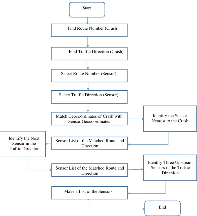
4.3.1 Sensor Identification ... 54
4.3.2 Traffic, Weather, and Roadway Geometry Data Identification ... 58
4.4 Descriptive Analysis of the Selected Crashes ... 67
4.5 Variables Transformation ... 70
Analysis and Results ... 73
5.1 Logistic Regression Models ... 74
5.2 Random Forest Models ... 84
5.3 Support Vector Machine Models ... 92
5.4 Models Comparison ... 98
Summary, Conclusions, and Recommendations ... 106
6.1 Executive Summary ... 106
6.2 Significant Findings ... 111
6.2.1 Logistic Regression Models ... 111
6.2.2 Random Forest Models ... 113
6.2.3 Support Vector Machine Models & RF+SVM Models ... 114
References ... 120
Appendix A - R Codes used for Model Development ... 132
Appendix A.1. 1: R codes of Logistic Regression Model ... 132
Appendix A.1. 2: R codes of Random Forest Model ... 134
List of Figures
Figure 1.1 Rural vs urban crash trends in Kansas (2012–2016) ... 3
Figure 1.2 Rural vs urban fatal crashes in Kansas (2012–2016) ... 3
Figure 3.1 Decision tree (courtesy of Mohd. Noor Abdul Hamid, Universiti Utara, Malaysia) .. 28
Figure 3.2 Random forest tree ... 29
Figure 3.3 Random forest voting process ... 31
Figure 3.4 Graphic representation of the SVM model (courtesy of (Z. Li et al., 2012)) ... 34
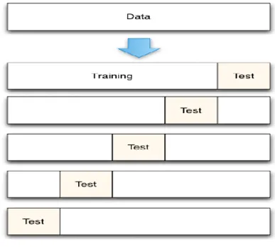
Figure 3.5 An example of five-fold cross-validation ... 38
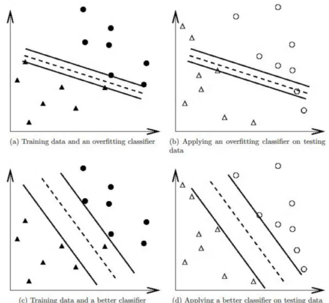
Figure 3.6 Overfitting classifier and a better classifier (courtesy of (Yang et al., 2015)) ... 39
Figure 3.7 ROC curve (courtesy of (C. Xu et al., 2013)) ... 41
Figure 4.1 Aggregation of database system ... 44
Figure 4.2 KDOT motor vehicle accident report ... 46
Figure 4.3 KC Scout system in Kansas City, Kansas ... 48
Figure 4.4 Flowchart of sensor sequence identification ... 57
Figure 4.5 Layout of KC Scout data request page (Courtesy of KC Scout Data Portal) ... 62
Figure 4.6 Layout of KC Scout query output page (Courtesy of KC Scout Data Portal) ... 63
Figure 4.7 Flowchart of matching traffic data with sensor data ... 65
Figure 4.8 Distribution of selected crashes during the study period... 68
Figure 4.9 Distribution of selected crashes against the days ... 68
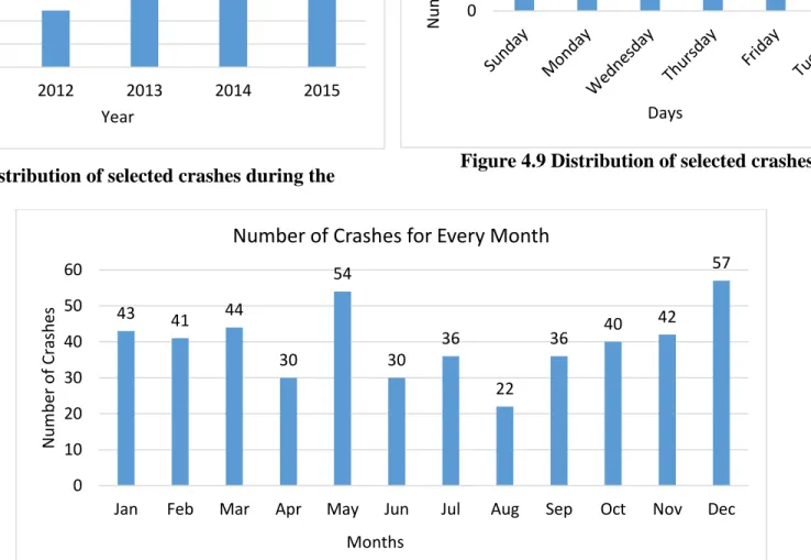
Figure 4.10 Distribution of selected crashes against the months ... 68
Figure 5.2 Optimum cutoff value selection (60:40 split) ... 78
Figure 5.3 Prediction accuracy of logistic regression models (60:40 split) ... 79
Figure 5.4 Prediction accuracy of logistic regression models (70: 30 split) ... 79
Figure 5.5 Prediction accuracy of logistic regression models (80:20 split) ... 79
Figure 5.6 Prediction accuracy of logistic regression on test data ... 79
Figure 5.7 Model sensitivity based on the split ratios ... 82
Figure 5.8 Model sensitivity based on the datasets... 82
Figure 5.9 ROC curve of log 1:2 model (80:20 split ratio) ... 83
Figure 5.10 Selection of optimal mtry parameter for random forest model ... 85
Figure 5.11 Selection of optimal maxnodes parameter for random forest model ... 85
Figure 5.12 Selection of optimal ntree parameter for random forest model ... 86
Figure 5.13 Variable importance plot ... 87
Figure 5.14 Prediction accuracy of random forest models (60:40 split)... 89
Figure 5.15 Prediction accuracy of random forest models (70: 30 split)... 89
Figure 5.16 Prediction accuracy of random forest models (80:20 split)... 89
Figure 5.17 Prediction accuracy of random forest models on test data ... 89
Figure 5.18 Sensitivity of the random forest models based on the dataset ... 91
Figure 5.19 Sensitivity of the random forest models based on the split ratio ... 91
Figure 5.20 Prediction accuracy of SVM models (60:40 split) ... 94
Figure 5.21 Prediction accuracy of SVM models (70:30 split) ... 94
Figure 5.22 Prediction accuracy of SVM models (80:20 split) ... 94
Figure 5.23 Prediction accuracy of test data using SVM models ... 94
Figure 5.25 Prediction accuracy of RF+SVM models (70:30 split) ... 95
Figure 5.26 Prediction accuracy of RF+SVM models (80:20 split) ... 95
Figure 5.27 Prediction accuracy of test data using RF+SVM models ... 95
Figure 5.28 Sensitivity of the SVM models based on the dataset ... 97
Figure 5.29 Sensitivity of the RF+SVM models based on the dataset ... 97
Figure 5.30 Sensitivity of the SVM models based on the split ratio ... 97
Figure 5.31 Sensitivity of the RF+SVM models based on the split ratio ... 97
Figure 5.32 Accuracy and sensitivity of all the models (60:40 split) ... 99
Figure 5.33 Accuracy and sensitivity of all the models (70:30 split) ... 99
List of Tables
Table 1.1 Traffic fatalities and fatality rates for 2016 (NHTSA, 2018) ... 2
Table 3.1 Sensitivity and specificity ... 40
Table 4.1 Kansas crash data ... 47
Table 4.2 Kansas reportable crashes ... 47
Table 4.3 Weather variables reported by NOAA ... 51
Table 4.4 Roadway geometry variable categories ... 52
Table 4.5 Sequence of the sensor IDs for each route and direction ... 56
Table 4.6 Temporal data points for each crash incident (only shown for VPH and for C sensor) 60 Table 4.7 Temporal and spatial data points for one crash incident (only shown for VPH and at the crash time) ... 64
Table 4.8 Weather variables for each crash incident (for all sensor) ... 66
Table 4.9 The new variables from the ‘Modified Dataset’ (only shown for VPH and at the crash time) ... 70
Table 4.10 Number of observations in each split ratio ... 72
Table 5.1 Stepwise regression output of 1:2 ratio of the modified dataset (60:40 split) ... 75
Table 5.2 Summary of logistic regression model (1:2 ratio) of the modified dataset (60:40 split) ... 76
Table 5.3 Optimum cutoff values for class prediction ... 77
Table 5.4 Logistic regression model accuracy ... 80
Table 5.5 Sensitivity and specificity of the logistic regression models ... 81
Table 5.6 AUC values of the logistic regression models ... 84
Table 5.7 Accuracies of the random forest models ... 88
Table 5.8 Sensitivity and specificity of the random forest models ... 90
Table 5.9 Accuracy of training and testing data from the SVM models ... 93
Table 5.10 Sensitivity and specificity of the SVM and RF+SVM models ... 96
Acknowledgments
The completion of this study would not have been possible without the expertise and support of my advisor Dr. Eric Fitzsimmons. I would also take this opportunity to thank my committee member Dr. William Hsu for sharing his insights on different sections of the analysis. I am grateful to Dr. Sunanda Dissanayake, who helped during the project selection and guided me in the right direction. I also thank the Kansas Department of Transportation for sharing the data used in this analysis. The analysis would not have been possible without the data from KDOT.
I would also like to thank Yeling Hu, Lei Luo, and Sandeep Dasari from the Department of Computer Science for providing help during data processing. Special thanks to my colleagues Blake Moris, Peng Wang, Jack Cunningham, and Benjamin Nye, for their help over the years.
I am indebted to my wife Sadia and daughter Arya for their unconditional support over the years. I would also like to acknowledge my mother and siblings for their encouragement and supports.
Introduction
1.1 Background
Traffic Crashes negatively impact communities and highway agencies throughout the world. In fact, in 2010, the World Health Organization (WHO) reported road injury as the tenth leading cause of death worldwide, increasing to the eighth leading cause of death in 2016 as the number of vehicles on roadways increased (WHO, 2018). In 2016, crashes accounted for
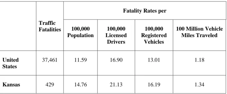
approximately 1.3 million deaths worldwide (WHO, 2018). The Centers for Disease Control and Prevention (CDC) reported that vehicle crashes were responsible for more than 32,000 fatalities in the United States in 2013, or 10.3 fatalities per 100,000 people, the highest fatality rate among similarly developed countries (CDC, 2016). According to the National Highway Traffic Safety Administration (NHTSA), approximately 37,461 deaths in the United States were attributed to vehicle crashes in 2016, while the Kansas Department of Transportation (KDOT) reported that 429 drivers and passengers were killed on Kansas roadways in the same year (approximately 1.1% of the national total). NHTSA reported that, compared to the national average, Kansas has a higher vehicle fatality average when the data are normalized (NHTSA, 2018). Table 1.1 compares national fatality rates and fatality rates for Kansas per population, number of licensed drivers, number of registered vehicles, and vehicle miles traveled. The fatality rates per 100,000 people and licensed drivers in Kansas are much higher than the national average. Additionally, 16.19 fatalities are reported per 100,000 registered vehicles in Kansas, whereas, the average is only 13.01 in the U.S. Fatalities per 100 million vehicles miles traveled in Kansas is 1.34, which is higher than the average of 1.18 across the U.S.
Table 1.1 Traffic fatalities and fatality rates for 2016 (NHTSA, 2018)
Traffic Fatalities
Fatality Rates per 100,000 Population 100,000 Licensed Drivers 100,000 Registered Vehicles 100 Million Vehicle Miles Traveled United States 37,461 11.59 16.90 13.01 1.18 Kansas 429 14.76 21.13 16.19 1.34
Since 2012, more than 60% of total vehicle crashes in Kansas, approximately 35,000 crashes per year, have occurred in urban areas (Figure 1.1). Among these crashes, 8.4% occurred on urban interstates and crashes on the urban principal and minor arterial roadways combined to account for 39.4% of total crashes in Kansas. Consequently, crash minimization in urban areas would reduce the total number of vehicle crashes throughout the state. Although urban crash rates are higher than rural crash rates, rural crashes have higher fatality rates since most urban crashes result in property damage only (PDO), crashes over $1000 in cost. In 2016, KDOT reported 48,095 PDO crashes and 13,365 injury crashes, resulting in 18,406 injuries. Figure 1.2 shows that rural roadways were responsible for more than 70% (231) of fatal crashes in Kansas in 2016.
Figure 1.1 Rural vs urban crash trends in Kansas (2012–2016)
Figure 1.2 Rural vs urban fatal crashes in Kansas (2012–2016)
0.00% 20.00% 40.00% 60.00% 80.00% 100.00% 120.00% 0 5000 10000 15000 20000 25000 30000 35000 40000 45000 2012 2013 2014 2015 2016 P erc entag e of Cr ashe s Numbe r of Cr ashe s Year
Rural vs Urban Crashes in Kansas
Rural (%) Urban (%) Rural Urban
0 50 100 150 200 250 300 2012 2013 2014 2015 2016 Numbe r of F atal C ra she s Year
Rural vs Urban Fatal Crashes in Kansas
Vehicle crashes also have significant economic impacts, including lost wages, medical expenses, and loss of workforce productivity. NHTSA reported a $242 billion direct economic loss, or 1.6% of the U.S. gross domestic product, due to vehicle crashes in 2010, and estimated a $594 billion indirect economic loss due to loss of life and decreased quality of life (NHTSA, 2015). NHTSA also estimated that vehicle crashes in Kansas in 2010 resulted in a $2.445 billion economic loss, a loss that increases annually due to inflation and increasing numbers of crashes (NHTSA, 2015).
Previous transportation studies have shown that traffic characteristics, weather
conditions, geometric design, and human behavior are common primary factors affecting a crash occurrence. Various studies have developed the relationship between crash severity and these factors, and other studies have predicted crash frequency based on these factors, but not in real-time. However, real-time crash prediction, defined as the prediction of an imminent crash event, could significantly decrease the number of vehicle crashes. Real-time crash prediction can be defined as the prediction of a crash event going to happen in the near future. Real-time
predictions must be made 5, 10, 15, or 30 minutes before a crash occurs so traffic management authorities can take preventive measures to diffuse a potential crash situation. Authorities involved with traffic management should be given enough time to handle the situation before a crash happen. Because real-time crash prediction is dependent on real-time traffic data, the availability of real-time data from Kansas City urban highways determined the roadway segments used for this study. KC Scout, a Kansas and Missouri bi-state traffic management system, collects traffic data on major highways in the Kansas City area, including average speed,
Researchers worldwide have utilized a variety of methods to study crash occurrences. Some studies have focused on real-time traffic flow predictions (Golob & Recker, 2003); others have concentrated on crash injury severity predictions (M. A. Abdel-Aty & Abdelwahab, 2004). Researchers have recently begun to study real-time crash predictions using machine learning approaches. One important practical implication of real-time crash prediction models is the identification of hazardous traffic conditions that may lead to a crash (Hossain & Muromachi, 2011). These models may also improve traffic operation efficiency and traffic safety as well as allow evaluation of operations using traffic congestion data and the study of traffic safety via crash analysis. The study of crash variables such as traffic, weather, and geometric conditions prior to a crash may provide insight that could be used for future crash predictions. The rapid advancement of intelligent transportation systems (ITS) in the past decade has enabled traffic agencies to collect traffic parameters such as traffic volume, speed, and occupancy in real-time. This traffic data is advantageous if properly analyzed and utilized in proactive or advanced traffic management systems. Many states are using variable speed limits (VSL) (Lee, Hellinga, & Saccomanno, 2006) and ramp metering (Lee, Hellinga, & Ozbay, 2006) to improve traffic safety.
Real-time crash prediction is still a relatively new field of traffic safety research, with only limited research in real-time crash prediction. Previous studies have focused specifically on traffic data, weather data, or geometric data, but this study is the first to combined weather, geometric, crash, and traffic data in time crash prediction. The next section describes real-time crash predictions and the methodology of previous real-real-time crash prediction related researches.
1.2 Real-Time Crash Prediction Modeling
Real-time crash prediction can be summarized as an approach to predict crashes based on real-time traffic data (Hossain & Muromachi, 2009). The term was first used in an academic research paper in 1995 (Madanat & Liu, 1995). Previous studies had estimated crash likelihood using traffic, vehicle, and human factors, but this study included environmental factors in the model to estimate crashes in real-time. Bayesian-type incident detection algorithms were applied for incident-likelihood predictions. Study results showed that accounting for environmental factors increases the accuracy of the likelihood estimates, and combining model predictions with traditional traffic measurements reduces incident detection times.
A later study used real-time traffic data from inductive loop detectors to estimate the likelihood of traffic crashes on freeways (C. Oh et al., 2001). Results showed that one unstable factor, such as environment, traffic conditions, vehicle, or human behavior, makes the traffic flow unstable and leads to a crash; therefore, pre-crash traffic dynamics may provide information regarding that crash. However, because human behavior heavily influences traffic behavior but human factors cannot be predicted accurately with mathematical models, so real-time crash prediction approaches have assumed that traffic flow data are the indirect representation of human factors (Hossain & Muromachi, 2009).
A study in 2003 developed a probabilistic real-time crash prediction model to estimate the crash potential of various traffic flow characteristics (Lee et al., 2003). The study introduced and defined crash precursors as traffic conditions that exist prior to a crash event. The study
crash precursors to estimate crash risk in real time. Identification of crash precursors is essential for accurate real-time crash prediction since misinterpretation of crash precursors may lead to erroneous prediction results.
The accuracy of real-time crash prediction models also depends on the selection of appropriate input variables. A study in 2006 developed a crash-likelihood model using real-time traffic flow data and rain data prior to and during a crash (M. A. Abdel-Aty & Pemmanaboina, 2006). The study accurately predicted 59% of the crash data. A rainfall index based on historical rain data demonstrated a positive impact on crash probability. Another study in Minnesota captured video of 110 live crashes, including traffic and weather conditions prior to and during the crash event (Hourdos et al., 2006). A crash-likelihood model, developed using the binary logistic regression model, identified the relationships between real-time traffic conditions and crash likelihood. Speed variability, lighting, and sun position were confirmed to affect crash likelihood. The model was tested on real-time data, and 58% of the crashes were detected accurately.
A study in 2009 investigated use of the statistical approach versus artificial intelligence on time crash prediction (Hossain & Muromachi, 2009). The study concluded that a real-time crash prediction model should have model calibration flexibility, fast prediction capability, and high model accuracy. The study also compared prediction accuracy based on artificially generated data, revealing that the Bayesian network predicted 18% more crash-prone conditions than the logistic regression model. As mentioned, previous research of real-time crash
predictions was based on traditional or modified statistical approaches. In the last decade, however, many researchers have begun utilizing artificial intelligence and machine learning
algorithms for real-time crash predictions due to their rapid computational ability and high prediction power.
1.3 Study Objectives
The objective of this research was to evaluate the application of the common statistical approach and machine learning algorithms on real-time crash prediction using real-time traffic
data and other variables. Logistic regression, random forest, support vector machine (SVM), and a hybrid combination of random forest and SVM were utilized. Logistic regression is commonly used in various aspects of traffic studies, and recently new machine learning techniques have shown promises as an overall classifier. Classification models can be used for real-time crash predictions to verify their ability to classify crashes accurately. These models were tested using fused data (traffic operations, roadway geometry, and weather) from the KC Scout traffic operations center, KDOT, and the National Oceanic and Atmospheric Administration (NOAA). A review of the literature showed that machine learning algorithms are being introduced into various aspects of transportation studies. A model with increased prediction accuracy can provide a better understanding of crashes, which may help with crash reduction, incident management, and identification of crash-prone locations.
Four secondary objectives were also identified:
Primary Objective: Evaluation of three machine learning algorithms’ application in real-time crash predictions.
• Develop predictive models for real-time crash predictions
• Develop a hybrid model of random forest and SVM
• Compare the machine learning algorithms for crash prediction
1.4 Thesis Outline
Following this introduction, Chapter 2 contains a review of the literature focused on real-time crash predictions. Based on the literature review, matched case-control logistic regression, SVM, and random forest methods are often used for real-time crash prediction. Chapter 2 also reviews the use of three proposed methods for various aspects of transportation safety and real-time crash prediction and justifies the use of the proposed methods. Chapter 3 presents the methodology of each proposed statistical method, including details of each methodology and its interpretation. The comparative parameters are also discussed, and the receiver operating curve (ROC), measurement of accuracy, and sensitivity analysis are used to compare the proposed models. Chapter 4 describes the methodology, including the data collection procedure, and a framework for future work. Chapter 5 includes a sample analysis with three preliminary models developed with a small sample data set to confirm that the proposed models have predictive power. The results are interpreted to draw conclusions from the sample analysis. Chapter 6 explains the scientific contribution of this study, including technology transfer and how agencies can efficiently utilize study findings.
Literature Review
Many studies have investigated crash prediction and crash severity, and various statistical approaches have been proposed and studied. Researchers commonly use binary/multinomial logit, ordered probit, and nested logit models (Miaou & Lum, 1993; Ossenbruggen et al., 2001; Shankar et al., 1996); neural networks (Abdelwahab & Abdel-Aty, 2001); fuzzy ARTMAP (M. A. Abdel-Aty & Abdelwahab, 2004); the log-linear model (Kim et al., 1995; Lee et al., 2003); the nonparametric Bayesian model (J.-S. Oh et al., 2005); discriminate analysis (Chengcheng Xu et al., 2013); the multivariate statistical model (Golob & Recker, 2003); and matched case-control logistic regression (M. A. Abdel-Aty & Abdelwahab, 2004; Hossain & Muromachi, 2011; Zheng et al., 2010). However, recent studies have utilized machine learning algorithms, and artificial intelligence to predict crash risks related to crash factors and traffic flow
characteristics (Chong et al., 2005; X. Li et al., 2008; Yuan & Cheu, 2003). The following sections broadly discuss the application of traditional statistical methods and machine learning methods in traffic safety studies, including real-time crash predictions.
2.1 Logistic Regression Models
Regression models have been widely used in traffic safety for many years, and transportation researchers have often applied various forms of logistic regression for crash analysis, injury severity analysis, and identification of crash contributing factors. Binary logistic regression and multinomial logistic regression are the most commonly used approaches (Donnell & Mason, 2004). Researchers have also used matched case-control logistic regression (M.
Miaou et al. analyzed two linear regression models and two Poisson regression models to investigate the relationship between traffic crashes and highway geometric designs. They
concluded that conventional linear regression models lack distributional properties that properly define random, discrete, nonnegative, and generally sporadic traffic crashes; therefore,
probabilistic statements and test statistics from linear regression models are doubtful. Poisson regression models, however, allow better relationships between crash events and other variables even though overdispersed data may overstate or understate the likelihood of traffic crashes on roadways (Miaou & Lum, 1993).
Kim et al. developed a log-linear model to identify the relationship between driver characteristics, crash severity, and injury severity. Odds multipliers were calculated from the model to estimate if certain variables increase or decrease the odds of severe crash or injury. Results showed that driver age and gender are not strong predictors of crash or injury severity. However, young drivers tend to engage in behaviors associated with more severe crashes and injuries. Alcohol and drug usage were shown to contribute to severe crashes significantly, and lack of seatbelt usage was shown to increase the odds of severe injuries in a crash (Kim et al., 1995).
Shankar et al. analyzed crash severity likelihood using nested logit formulation. Four levels of injury severity were used in the prediction model: PDO, possible injury, evident injury, and disabling injury or fatality. A 61-km section of rural interstate in Washington state was used for analysis, and data were collected over a 5-year period. Roadway geometry, weather, and human factors were found to be significant factors for developing a probabilistic model (Shankar et al., 1996).
Ossenbruggen et al. used logistic regression to identify statistically significant factors associated with crash and injury severity Results showed that land use activity, presence of sidewalks, traffic control device usage, and traffic flow are the most significant factors that determine if a site is more hazardous than other sites. Of the three types of sites studied (village, shopping, and residential areas), residential and shopping sites were shown to be more hazardous than village sites because village sites typically have low operating speeds and
pedestrian-friendly areas (Ossenbruggen et al., 2001).
Oh et al. initially investigated the relationship between real-time traffic parameters and crash incidents. They developed a Bayesian model with traffic data (average and standard
deviation of traffic flow, occupancy, and speed at 10-seconds intervals). The data consisted of 52 crashes, and traffic conditions were categorized as normal traffic conditions or disruptive traffic conditions. Normal traffic condition is a 5-minutes period that occurs 30 minutes before the crash incident; disruptive traffic condition is the 5-minutes period right before a crash event. Study results showed that a 5-minutes standard deviation of speed is a significant variable that can be used to estimate crash likelihood. Although only a small sample size was used in the analysis, a relationship between traffic parameters and the crash prediction was evident (C. Oh et al., 2001).
Bedard et al. developed a multivariate logistic regression model to determine the contributions of driver, crash, and vehicle characteristics to driver fatality risks. Data from the Fatality Accident Reporting System (FARS) for single-vehicle crashes involving fixed objects were used for analysis. The study reported an odds ratio of 4.98 for drivers over 80 years old
Increasing seatbelt usage, reducing speed, and reducing the number and incident of driver-side impact was shown to potentially prevent fatalities (Bedard et al., 2002).
Sohn et al. used algorithms to investigate the relationship between crash severity and environmental driving factors. They applied classifier fusion, ensemble, and the clustering method to improve the classifier for two categories of crash severity in Korea. The neural network and decision tree had previously been used as classifiers. Results showed that
classification-based clustering performs better if observation variation is relatively large (Sohn & Lee, 2003).
Lee et al. proposed a probabilistic log-linear model to predict real-time crashes based on traffic flow characteristics. The study suggested a rational method to identify crash precursors based on experimental results and then tested the performance of the crash prediction model. They used real-time traffic flow data to explain traffic performance characteristics during crash events. Crash frequency was a function of traffic and environmental characteristics, external factors, and exposure. The authors identified three parameters as crash precursors: average variation of speed difference across adjacent lanes, traffic density, and difference of speeds at upstream and downstream ends of road sections. The study found that the speed difference between the upstream detector and the downstream detector was significantly higher during the crash. In addition, the study concluded that abrupt speed drops at the upstream detector are a significant parameter for real-time crash predictions. However, the effect of the average variation of speed across adjacent lanes was found to be insignificant (Lee et al., 2003).
Another study used nonlinear canonical correlation analysis to find a pattern between crash characteristics and traffic flow characteristics while controlling for lighting and weather
parameters. They also compared the nonlinear canonical analysis method to the principal
component analysis method using three data sets: segmentation by lighting and weather, accident characteristics, and traffic flow characteristics. Results showed that collision type is related to median speed, and lane variations of speed and that crash severity is inversely related to the traffic volume. Study results suggested that moderate traffic and relatively constant speed can lead to increased crash severity (Golob & Recker, 2003).
A study in Pennsylvania used logistic regression models to predict the severity of median-related crashes. Researchers developed models to predict the probabilities of fatal, injury, and PDO crashes. Traffic operations, geometric conditions, and weather conditions were used as independent variables to determine their relationship to crash severity. The study found that the presence of curvilinear alignment and drivers’ use of drugs or alcohol increases the chance of fatality in a cross-median crash. In addition, the presence of an interchange entrance ramp, roadway surface conditions, and traffic volume increases the severity of a median crash. Study results concluded that the geometric design of the roadway must be considered in real-time crash prediction to increase prediction accuracy (Donnell & Mason, 2004).
One study used matched case-control logistic regression to explore the effects of traffic flow parameters on the effects of other confounding variables (i.e., location, time, and weather). Every crash in a matched case-control study is considered a case, and every non-crash event is a control. Loop detectors on Florida freeways collected the data used in this study. The 5-minutes average occupancy and 5-minutes coefficient of variation in the speed at the upstream and downstream stations (5–10 minutes before the crash) were found to be the most significant
Zheng et al. used case-controlled data to similarly develop a matched case-control logistic regression model to estimate the impacts of speed variance from oscillating traffic state on the likelihood of crash occurrence using case-controlled data (Zheng et al., 2010).
Hossain and Muromachi developed a Bayesian network-based crash prediction model for ramp vicinities and basic freeway segments, reporting a unique set of contributing factors for each area. The mean and the difference between standard deviations of traffic flow between adjacent lanes were found to be significant factors for higher crash risk in basic freeway segments, whereas variation in speed between upstream and downstream detector stations was found to be the most significant factor in ramp vicinities (Hossain & Muromachi, 2011, 2012).
Although traditional statistical approaches are often used in transportation studies related to crash injury severity analysis and crash detection analysis, they require assumptions about data distribution and usually a linear function form between response and independent variables (Z. Li et al., 2012). Violations of these assumptions may lead to erroneous estimation and incorrect inferences (Mussone et al., 1999).
Therefore, researchers have proposed non-parametric methods and machine learning methods for real-time crash prediction and crash injury severity analysis. A primary advantage of using machine learning models is that they do not require a predefined underlying relationship between response and independent variables. In previous studies, researchers have reported that non-parametric studies provide a better statistical fit than traditional parametric models (de Oña et al., 2011; Fish & Blodgett, 2003).
2.2 Machine Learning Algorithms
Researchers have recently begun applying machine learning algorithms to significant variables in order to analyze traffic crashes (Abdelwahab & Abdel-Aty, 2001; Chong et al., 2005; Z. Li et al., 2012) . Machine learning algorithms are also being used for crash prediction (M. M. Ahmed & Abdel-Aty, 2012a; Qu et al., 2012, 2012; C. Xu et al., 2013). Due to their efficiency in dealing with classification and regression problems, two non-parametric models, random forest and SVM, have recently been used in real-time crash prediction studies (Z. Li et al., 2012). Random forest is an efficient technique for variable evaluation and importation ranking, as well as crash prediction. Previously, the random forest had been used to identify significant variables (Harb et al., 2009; Hossain & Muromachi, 2011) and traffic flow prediction (Hamner, 2010). However, the random forest can also be used for prediction in new data (Beshah et al., 2011; Krishnaveni & Hemalatha, 2011). SVM has been used in transportation studies, including traffic flow prediction (Cheu et al., 2006; Zhang & Xie, 2008), incident detection (Yuan & Cheu, 2003), travel mode choice modeling (Zhang & Xie, 2008), crash frequency prediction (X. Li et al., 2008), crash injury severity analysis (Z. Li et al., 2012), and real-time crash prediction (Qu et al., 2012; Yu & Abdel-Aty, 2013, 2014).
Abdelwahab et al. used two artificial neural network methods, multilayer perceptron, and fuzzy adaptive resonance theory, to investigate the relationship between driver injury severity and driver, vehicle, roadway, and environmental characteristics. Traffic crashes at signalized
and testing data sets, respectively, in the multilayer perceptron model, and the fuzzy adaptive resonance theory was shown to provide a classification accuracy of 56.2% (Abdelwahab & Abdel-Aty, 2001).
Despite their high classification accuracies, however, neural networks require a large number of hyperparameters, neural network results are not reproducible due to randomness, and computation time is usually higher than other models. In addition, neural networks have shown an overfitting tendency. As a result, researchers have started using advanced machine learning methods such as random forest, SVM, classification and regression tree (CART), and
discriminant analysis. Although each method has advantages and disadvantages, based on a thorough literature review and study of prediction and interpretation powers, random forest and SVM were chosen for this study.
2.2.1 Random Forest
A majority of random forest traffic safety studies have identified significant variables that were then used to develop other models. Harb et al. conducted one of the first applications of the random forest to explore pre-crash maneuvers using classification trees and random forest. The random forest technique was used to determine the importance of independent variables’ rankings for various accident types. The researchers chose to use a random forest because it can extract variable importance information that is not readily available in the classification tree method. Although output from the classification tree may provide important variable rankings, the variables may be correlated with each other, leading to misinterpretation of the results. Therefore, after analyzing the data using the classification tree method, the variables were ranked
using the random forest for various types of crashes, including angle accidents, head-on collisions, and rear-end accidents (Harb et al., 2009).
The random forest method has also been used to predict travel times by modeling local and aggregate traffic flow. One study attempted to predict future traffic flow in order to predict approximate future travel time. The random forest method was employed to predict future traffic speeds from the training data (Hamner, 2010).
A study in Portugal used the random forest to identify highway rear-end crash risk using disaggregated data. The study classified traffic situations as non-crash and pre-crash using the random forest method. A threshold between 0 and 1 was defined to classify pre-crash and non-crash scenarios. If the predicted output fell below the threshold value, the response was classified as a non-crash event, and if the likelihood was greater than the threshold, the response was recorded as a pre-crash event. The research used a 67:33 ratio of the data for the training and test sets. The training set was used to develop the model, and the test set was used to evaluate model performance. The results accurately predicted 81.1% of pre-crash and 86.7% of non-crash events after data calibration. The variable importance ranking showed that speed variations in the right lane, the speed difference between two adjacent lanes, and the left lane’s standard deviation of headway are critical factors for rear-end crashes in various highway traffic conditions (Pham et al., 2010).
The random forest has also been utilized for real-time crash prediction and explaining crash mechanisms in urban expressways. Basic freeway segments and ramp segments were analyzed using 32 and 31 independent variables, respectively. Data from one upstream and one
vehicle count, 5-minutes average occupancy, 5-minutes SD of speed, count, and occupancy data were collected in addition to other traffic-related data (Hossain & Muromachi, 2011).
Very few transportation studies have used the random forest for prediction, but one such study employed random forest for the classification of variables in traffic crashes using traffic data from the transport department of Hong Kong. The study analyzed one data set using five machine learning methods: naive Bayes, adaptive boosting, decision tree, partial decision tree, and random forest. Results showed that random forest outperformed the other four methods in the classification of variable levels. A similar approach could be used to classify crash and non-crash events (Krishnaveni & Hemalatha, 2011).
Another study utilized random forest for pattern recognition and increased understanding of traffic crash data. The study compared the performance of CART and random forest methods for classifying injury severity level. A binary response was used for classification. Random forest accurately predicted 73.45% of injury severity and 99.74% of PDO crashes, and the random forest technique produced a lower error rate than the CART model. The values of the area under the curve (AUC) in a ROC curve were 0.8873 and 0.9000 for the CART model and the random forest model, respectively. However, both models more accurately predicted PDO crashes over injury crashes (Beshah et al., 2011). The study did not report the reason behind the improved prediction, but the inference can be made that the proportion of injury and PDO data may play a role. Other studies also showed that the models more accurately predict PDO crashes than injury-related crashes, a fact that should be considered during data set selection. Previous studies also reported that common contributing factors, such as a large speed difference between adjacent lanes (M. Ahmed et al., 2012a; Hossain & Muromachi, 2012) and compression waves
that abruptly change traffic flow (M. M. Ahmed & Abdel-Aty, 2012b), increase the likelihood of traffic crashes.
2.2.2 Support Vector Machine
Yuan et al. initially employed the SVM method for incident detection and incident classification. They used three nonlinear-based kernel functions (radial, polynomial, and linear), and a model was built by separating the data into testing and training sets. However, the linear kernel was still able to be used with other data sets since data distribution may significantly affect kernel performance. The linear SVM failed to classify incidences from non-incidences. Study results showed that the SVM has a low misclassification rate, high accuracy in incident detection, low false alarm rate, and faster detection time than the neural network method (Yuan & Cheu, 2003).
Chong et al. examined four machine learning techniques to find an accurate model for injury severity prediction. The four examined models were artificial neural network using hybrid learning, decision trees, SVMs, and hybrid decision tree-artificial neural network. They were among the first to analyze five classes of injury severity instead of just two classes
(injury/fatality versus no injury) as in traditional studies. Crash data were collected from the General Estimates System (GES) from 1995 to 2000. Each model showed different accuracies when classifying each level of severity. The decision tree predicted no injury and possible injury classes more accurately, but the hybrid approach more accurately classified non-incapacitating injury, incapacitating injury, and fatal injury classes (Chong et al., 2005).
studies. Two models were developed and compared based on data from approximately 2000 crashes on rural frontage roads in Texas. Study results showed a more accurate performance for the SVM model than the negative binomial regression model and the neural network model. The SVM model is advantageous because it does not overfit the data, which is a common problem when applying negative binomial regression (X. Li et al., 2008).
Li et al. used SVM and an ordered probit model to analyze crash injury severity on 326 freeway diverging areas. A radial basis function (RBF) kernel was used for the SVM model. Study results showed better prediction accuracy from the SVM model than the ordered probit model: SVM predicted 48.8% injury severity correctly, whereas the ordered probit model predicted 44%. The researchers also used sensitivity analysis to evaluate the effect of explanatory variables on crash injury severity. The analysis showed that ramp length and shoulder width of the freeway significantly affect injury severity in crashes on diverging ramps (Z. Li et al., 2012).
Yu et al. compared an SVM model and Bayesian logistic regression model to evaluate their applications for real-time crash risks. The data set was categorized as training and test, and significant independent variables were selected via CART models. The CART models found average downstream speed, crash location average speed, crash location standard deviation of occupancy, and crash location standard deviation of volume as significant variables that were used to develop the prediction model. Two commonly used kernels, linear, and RBF, were considered for the model to compare kernel performance. The study concluded that the SVM model with the RBF kernel provided the best goodness-of-fit. In addition, the nonlinear
relationship between the response variable and independent variables was best explained with the SVM model with the RBF kernel. The study showed a promising application of SVM in traffic
safety for small sample sizes on newly built roadways or freeways with recently implemented ITS systems (Yu & Abdel-Aty, 2013).
Chen et al. used polynomial and RBF kernels to develop an SVM model to investigate driver injury severity in rollover crashes. They also utilized a CART model to identify significant variables. Study results showed that the polynomial SVM outperformed the RBF SVM and that a trained SVM classifier is most advantageous for no-injury events and least helpful for
incapacitating/fatal injury events. Sensitivity analysis used to interpret results from the SVM analysis showed that Driving Under the Influence (DUI) was the most significant variable as it causes incapacitating or fatal injuries. In addition, a large number of travel lanes, the use of a traffic control device, and unpaved roadways were shown to increase the severity of a rollover crash (Chen et al., 2016).
Based on the literature review, logistic regression was chosen to study because it is most commonly used, and random forest and SVM were evaluated because they outperformed other approaches in previous traffic safety studies. Chapter 3 details the procedures, advantages, and disadvantages of the selected methods.
Methodology
This chapter describes each selected model, including its procedures and how results are interpreted. The chapter also explains logistic regression model assumptions and modifications, including the variable selection procedure, as well as random forest and SVM model
development, including model procedures.
3.1 Logistic Regression
Logistic regression analysis is commonly used to analyze a binary response variable. The response variable used in logistic regression takes the form of success/failure (1/0), where ‘1’ generally denotes success, and ‘0’ denotes failure. The success/failure form can be changed to match any binary response (M. Abdel-Aty et al., 2004; Shankar et al., 1995; Yan et al., 2005). The general linear model assumes that responses and error terms are normally Gaussian
distribution, and the observations are independent (Hilbe, 2011). When binary data are modeled using this method, however, the first two assumptions are violated because the binary response variable is derived from Bernoulli distribution, whereas normal regression is based on the Gaussian probability distribution function (pdf).
Nelder and Wederbrum proposed the generalized linear model (GLM), which utilizes a single algorithm for estimating models based on the exponential family of distributions. GLM methods are commonly used to estimate logistic, probit, and count response models, such as Poisson and negative binomial regression (Nelder & Wedderburn, 1972).
The logit, or natural logarithm of an odds ratio, is the central mathematical concept underlying logistic regression. The logistic model predicts the logit of Y from X. The odds can be
defined as the ratios of probabilities (π) of success of Y to probabilities of failure of Y. The simple logistic regression model can be written in the following form (Peng et al., 2002):
𝑙𝑜𝑔𝑖𝑡 (𝑌) = ln 𝜋
1−𝜋= 𝛽0+ 𝛽1𝑥1+ 𝛽2𝑥2+ ⋯ 𝛽𝑛𝑥𝑛 = 𝛽0+ ∑ 𝛽𝑖𝑥𝑖 , (3.1)
where π is the probability of success, x1…….xn represents independent variables in the
model, and β represents the regression coefficient for each variable. Once both sides of the equation are converted with antilog, the equation takes the following form:
𝜋 = 𝑃(𝑌 = 1) = 𝑒𝛽0+𝛽1𝑥1+𝛽2𝑥2+⋯𝛽𝑛𝑥𝑛
1+𝑒𝛽0+𝛽1𝑥1+𝛽2𝑥2+⋯𝛽𝑛𝑥𝑛, (3.2)
where π is the probability of success (Y = 1). Although Equation 3.1 presents a linear relationship between logit (Y) and X, Equation 3.2 shows the relationship between Y and X to be nonlinear. Therefore, the natural log transformation of the odds must be used to make a linear relationship between categorical response and predictors. The β coefficient is used to interpret the direction of the relationship between X and logit (Y). A large β value (β > 0) means that the large logit (Y) is associated with large X values and vice versa. In contrast, small (β < 0) means that small logit (Y) is associated with large X values and vice versa.
The maximum likelihood method is often used to predict β in a logistic regression model to maximize the likelihood of reproducing the data given the parameter estimates. The null hypothesis for full models indicates that all βs are zero. If the null hypothesis is rejected, at least one β is not zero, which implies the logistic regression model predicts the probability of the outcome better than the mean of the dependent variables.
Final interpretations of the results are made using the odds ratio of the predictors (Peng, Lee, & Ingersoll, 2002). The odds ratio is a measure of association between an exposure and an outcome (Szumilas, 2010), as derived from exp (β); if an independent variable experience a one-unit increase with other factors remaining constant, then the odds ratio increases by a factor of
exp (β). An odds ratio greater than 1 (less than 1) represents exposure associated with higher (lower) odds of outcome for a unit increase in the independent variable. A 95% confidence interval of the odds ratio is also often used to evaluate the result; a large confidence interval represents a low level of precision. It can be used as a proxy to find statistical significance if the confidence interval does not include an odds ratio of 1 in the interval. The odds ratio can be used to compare levels of individual independent variables (Szumilas, 2010; Hosmer, Lemeshow, & Sturdivant, 2013).
3.1.1 Interpretation of Odds Ratio
• An odds ratio of 1 indicates no difference between groups and no association between tested levels.
• An odds ratio greater than 1 suggests that the odds of exposure are positively associated with the success rather than the failure.
• An odds ratio less than 1 indicates that the odds of exposure are negatively associated with the success as compared to the failure.
3.1.2 Variable Selection
The selection of the best subset of variables, which consequently increases accuracy, requires a proper variable selection method. Unnecessary variables in the model add noise to the
estimation. In addition, too many insignificant variables in the model cause collinearity and make the model difficult to explain. Prediction accuracy increases when insignificant variables are removed from the model. Common procedures used for variable selection in logistic regression are described in the following sections.
3.1.2.1 Backward Selection
Backward selection is the simplest of the variable selection methods used in logistic regression analysis. All variables are in the model at the beginning of the procedure, and then the variable with the highest p-value is removed, and the data is refitted. The procedure is repeated until no variables to remove, or all the variables have p-values smaller than the critical p-value. The critical p-value is defined before the procedure begins. The drawback of backward selection is that any of the removed variables could be significant in future steps when other variables are removed from the model.
3.1.2.2 Forward Selection
Forward selection starts with no variable in the model and then adds variables with p-values less than the critical p-value. The steps are repeated until no more variables with p-p-values lower than the critical p-value remain, ending the procedure. Variables selected during the process are used in the final model to fit the data.
3.1.2.3 Stepwise Selection
variable is dropped from the model. This procedure requires two critical values: one for variable selection and another to remove a variable from the model.
3.1.2.4 Akaike Information Criterion
Akaike information criterion (AIC) is a regression technique that selects a model based on how close its fitted values are to the true expected values. AIC can be defined as
AIC = -2 (log likelihood - number of parameters in model). (3.3)
The optimal model has the most fitted values close to the true expected probabilities (Agresti, 2003). However, AIC penalizes a model for including too many variables.
3.2 Random Forest
Leo Breiman proposed a supervised machine learning algorithm called ‘random forest’, also known as an ensemble approach, as a promising procedure for extracting rankings of variable importance. The random forest method can be used for both classification and
regression problems (Breiman, 2001). The main principle behind the ensemble method is that a group of weak learners can combine to build a strong learner. The method builds a forest, or ensemble, of decision trees often trained with the bagging method that combines learning models to increase the accuracy of the overall result. In other words, the random forest builds multiple decision trees and merges them together to obtain an accurate, stable prediction.
The random forest begins when a decision tree takes input at the top and uses different variables to travel down. As the tree grows, the size of the branches gets smaller. Decision trees can handle numerical and categorical data, and they demonstrate rapid performance on large data
sets. The root or topmost node of the tree is the decision node that splits the data set using a variable or feature, resulting in an evaluation of the best splitting metric or each subset or class in the data set. The decision tree learns by recursively splitting the data set from the root onwards. Each internal node represents a test on an attribute, each branch represents the test outcome, and each leaf node represents a class label. A node with no children is called a leaf. Figure 3.1 shows the components of a decision tree.
Figure 3.1 Decision tree (courtesy of Mohd. Noor Abdul Hamid, Universiti Utara, Malaysia)
Two well-known methods used in classification and regression problems are boosting (Schapire et al., 1998) and bagging (Breiman, 1996). Boosting gives extra weight to points incorrectly predicted from successive trees by earlier predictors. Bagging, however, does not depend on earlier trees because each tree is individually constructed using a bootstrap sample of the data set, and then a majority vote is taken for prediction (Liaw & Wiener, 2002). Random
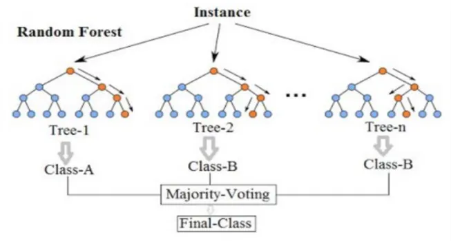
predictors randomly chosen at that node instead of splitting each node using the best split among variables as in standard decision trees. Decision trees are also prone to overfitting, especially when a tree is particularly deep, but trees in random forest are constructed based on a certain number of trees, and then results from all the trees are aggregated. Another disadvantage of the bagging tree method is that it uses the entire set of variables while creating splits, so if some variables are indicative of certain predictors, the forest could be comprised of correlated trees, thereby increasing biasness and reducing variance. Random forest aims to de-correlate and prune the trees by setting a stopping criterion for node splits. The random forest algorithm introduces extra randomness into the model while a tree is constructed, and instead of searching for the best variable when splitting a node, the algorithm, searches for the best feature among a random subset of features. This process creates diversity, which generally results in a better model as shown in Figure 3.2.
A random forest consists of a combination of classifiers where each classifier contributes a single vote for the most frequent class of the input vector (x) (Rodriguez-Galiano et al., 2012):
𝐶̂ = 𝑚𝑎𝑗𝑜𝑟𝑖𝑡𝑦𝑣𝑜𝑡𝑒 {𝐶𝑟𝑓𝐵 ̂(𝑥)}𝑏 𝐵, (3.4)
where 𝐶̂(𝑥)𝑏 is the class prediction of the random forest tree. Random forest increases randomness by building trees from training data subsets created by bagging or bootstrapping (Breiman, 1996). Bootstrapping aggregation creates a training data set by resampling original data with randomly chosen replacement data. Consequently, some data may be used more than once, while other data may never be used, leading to increased classifier stability (Breiman, 2001).
3.2.1 Random Forest Algorithm
The random forest algorithm consists of two steps. The first step creates the random forest, and the second step makes predictions from the created random forest. The process for the first step requires the following procedure:
1. Randomly select n features from total k features, where n << k. 2. Among the n features, calculate node d using the best split point. 3. Split the nodes into children nodes using the best split.
4. Repeat steps 1–3 until I number of nodes are reached.
5. Build forest by repeating steps 1–4 m number of times to create m number of trees. As shown in Figure 3.3, the second stage of the random forest requires the following steps:
2. Calculate votes for each predicted outcome.
3. Designate the highest voted predictors as the final prediction from the random forest algorithm.
Figure 3.3 Random forest voting process
3.2.2 Validation and Performance of Random Forest
CART selects the best set of predictors using a variety of impurity or diversity measures (e.g., Gini, twoing, ordered twoing, and least-squares deviation) (Kurt et al., 2008). The most commonly used metrics in the random forest are Gini impurity, which is used for classification problems, and variance reduction, which is used for regression problems (Degenhardt et al., 2017). Gini impurity is the measure of impurity of a set of variables; it calculates the probability of being wrong. The Gini impurity at node t, g(t) is defined as
where i and j are categories of the target variable. The Gini index equation can be written as
𝑔(𝑡) = 1 − ∑ 𝑝2(𝑗|𝑡)
𝑗 . (3.6)
Therefore, when node cases are evenly distributed across categories, the Gini index uses its maximum value of 1-(1/k), where k is the number of categories for the target variable. If all cases in the node belong to the same category, the Gini index equals 0 (Breiman, 2017; Kurt et al., 2008).
3.2.3 Mean Decrease Accuracy
The mean decrease accuracy index measures variable importance by permuting out-of-bag (OOB) error and computing the importance of the variables (Han et al., 2016). Breiman’s original implementation of the random forest algorithm trained each tree on approximately two-thirds of the training data (Breiman, 2001). Consequently, as the forest is built, each tree can be tested on the