Empirical modeling & Analysis of Tube Hydroforming process of Inconel 600 using Response Surface Methodology

Empirical modeling & Analysis of Tube

Hydroforming process of Inconel 600 using Response

Surface Methodology

B. Sreenivasulu

, Dr. G. Prasanthi

1 _{Assistant Professor, Department of Mechanical Engineering,}

Madanapalle Institute of Technology and Science, Madanapalle. Andhra Pradesh., INDIA. 2

Professor, Department of Mechanical Engineering, JNTUA College of Engineering, Anantapuramu, INDIA Email: [email protected]

Abstract— Tube hydroforming process (THFP) is one of new forming techniques having many applications in the area of automotive and aerospace industries due to its capability to produce very complex tubular parts in a single step. The other advantages of THFP are improved structural strength and stiffness, lighter products and less material wastage.

The main failures of THFP are bursting, buckling and wrinkling. These failures are to be avoided by proper selection of loading paths. The success rate of Hydroforming technique depends strongly on the selection of process parameter and the selection of loading path.

From literature survey and trial experiments, it is found that internal pressure, axial feed & Length of the tube has major effect on the accuracy of the process. Therefore, the internal pressure, axial feed and length of the tube are taken as the influencing variables and the range of these variables are found by conducting trail experiments on Inconel 600 tubes.

In consideration of the cost of process and materials, DOE (Design of experiments) is applied to minimize the total number of experiments required to complete the analysis with same accuracy. In continuation to that, the RSM (Response Surface Methodology) is applied to predict the mathematical models to estimate bulge ratio and thinning. Later the predicted models are utilized to optimize the tube hydroforming process.

Index Term— Tube Hydro forming process, Inconel 600, Response surface methodology.

1. INTRODUCTION

Automobile and aerospace industries are showing interest on THFP due to its capability to produce the complex tubular components in single phase with better mechanical properties. The components produced by THFP are structurally sound.

By the THF process, manufacturers are able to produce complex shaped parts with lightweight and fewer welds than alternative metal forming techniques.

The main benefit with THFP is to minimize the number of welds in the component and capable to fabricate the complex geometrical parts. The other merits of THFP over conventional metal forming process are diminution in product cost, tools cost, product weight, admirable utilization of material, fewer operations, and superior part quality, improved structural stability and stiffness [1].

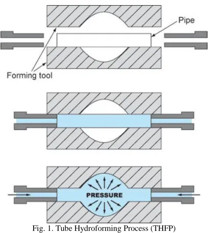
The major steps involved in THFP are placing a straight or pre-formed tube in a die, application of pressure

inside the tube and application of axial compressive force at two ends of the tube simultaneously, to deform into die to obtain die shape as illustrated in figure 1.The goal of THFP is to form the tubes to a desire shape with control of process parameter to avoid failures such as buckling, wrinkling, or bursting.

Fig. 1. Tube Hydroforming Process (THFP)

It is very much essential to study the effect of process parameters on product quality of the hydroformed part. Hence this process is chosen for investigation and further analysis. The main objective of the current investigation is to study the effect of process variables on hydroformability to improve the product quality.

formulation of objective function and can be solved using any evolutionary algorithms.

Fig. 2. Free Bulge Tube Hydroforming process.

Many of the researchers are working on development of THFP to make the process easy and convenient to industry. Honggang [2] et al, using square cross sectioned die for THFP, established a methodology to find the optimal process conditions.

Using LS-DYNA (FEA tool), simulations are conducted at various conditions to carry out the hydro-forming experiments. A sensitivity analysis was also carried out with analysis of variance. Necking/fracture, wrinkling, and thinning are considered as the parameters to formulate the multi objective function and RSM was used to find the most effective factor and to produce a defect-free hydroformed component. Carleer et al. [3] studied the effect of the anisotropy and hardening exponent on free expanded tubes and concluded that these factors having major effect on output responses. And also the anisotropy and friction have the considerable effect on strain distribution. Using Finite Element Method, Boudeau et al. [4] discovered the effect of material parameters and process conditions on process failures, such as necking and bursting. The quality of the hydroformed part depends on the geometry of the die. Ko and Altan [5] considered geometry of the die also as an influencing factor and studied the effect of process conditions along with geometrical parameters using 2D FEM tool and found that the pressure and length of the tube are the parameters showing major effect on the bulge of an axisymmetric part.

Yang et al. [6] investigated the effect of internal pressure and axial force on THFP and established a mathematical approach.

In economical point of view, conducting many number of trail experiments to investigate the effect of the process parameter on the process is more expensive. Due to this reason, to reduce the number of experiments without affecting quality of the analysis, Taguchi method was applied to metal forming area [7–10]. After considering the benefits of the Taguchi experimental design, in present research Taguchi L9 was selected for THFP analysis.

The proposed work is all about conducting the experiments by using Design of Experiments. Then using the experimental data modeling of the process is done with Response Surface Methodology (RSM). The models predicted using RSM is tested for its adequacy using ANOVA analysis. Based on the value of Regression Coefficient (R2), the models will be utilized further for optimization of the process. The effect of input process parameters on the output responses are

also plotted using Design Expert software. In this research work annealed INCONEL600 tubes are used for conducting experimentation. The novelty in this research is that only a few researchers worked on the super alloys.

2. EXPERIMENTAL WORK

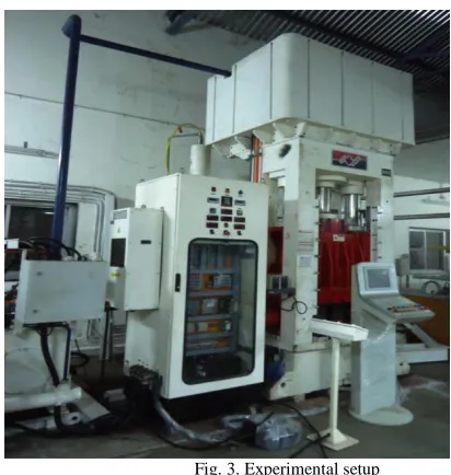
The experiments for the bulging of straight tube are performed by using the hydroforming press of capacity 200 tons, shown in figure 3. The setup was designed and developed by Electropneumatics and Hydraulics India Limited, pune. The tube hydroforming machine and the process variables such as pressure and axial feed to achieve the various loading paths during the operation can be controlled computer programming. The maximum dimeter of the die which can be accommodated is 57.15mm and length up to 300 mm for free bulge tube hydroforming. the setup having pressure intensifiers to get high pressure. The movement of the axial plungers can be controlled either independently or simultaneously. The free bulge tests as per the Taguchis L9 orthogonal array are carried out on the INCONEL 600.

Fig. 3. Experimental setup

INCONEL 600, which is a nickel based super alloy, is used as the work material due to its superior properties, such as resistant to corrosion, resistant to oxidation, and good tensile and creep properties. Inconel 600 alloy is widely used in gas turbines, rocket motors, space craft, nuclear reactors pumps and tooling. The chemical test was conducted to find the chemical composition of INCONEL 600 and is shown in Table I.

Table I

Chemical composition of annealed INCONEL 600

Element Ni Cr Fe Mn Cu Si S C

Percentage 72.31 16.54 9.90 0.14 0.017 0.4 0.001 0.012

Table II

Geometrical detail of the tube and die External Diameter of tube 57.00mm

Length of the tube 195, 210, 250 mm

Thickness 1.4mm

Table III

Properties of the tube material Tensile

test

0.2% proof load(K N)

Ultimat e load(K

N)

0.2% proof stress (MPa)

U.T.S (MPa)

Mod ulus (MP a)

%of elonga

tion

After Annealing

3.02 9.55 174 549 1530

84

41.64

The main objective of free bulging hydroforming process is to get the maximum bulge without any failures. The bulge ratio is one of the output responses and is specified by df/di. Thinning ratio is considered as another response. This study includes the variation of the thickness from initial tube thickness to the final thickness at the maximum bulge point. The thinning and the bulge ratio are selected as the quality characteristics. The thinning ratio is defined by

Thinning ratio=

Where t0is the original thickness of the tube and tf is the final thickness of the hydroformed tube at the bulge point as shown in Fig. 2. The bulge ratio is defined by

Bulge ratio=

Where df is the maximum bulge diameter of the hydroformed tube and di is the initial diameter of the tube as shown in Fig. 2.

From literature survey and the trail experiments, it is found that internal pressure, axial feed and Length of the tube are significant factors having major effect on the bulge ratio and thinning ratio. These three factors are considered as the decision variables and trial experiments were conducted on tube hydroforming equipment by varying one of the process variables to determine the working range of each process variable. The upper and lower limits of the factors were coded as +1 and -1 respectively. The coded intermediate values are calculated using the following relationship;





max min

2 2 ( )

( )

i

X X X

X

X X

 



 (1)

Here, Xmin and Xmax are lower and upper level of the variable respectively and Xi is the required coded value of a variable X. X is any value of the variable between Xmin to Xmax. Table IV includes the process parameters, units, notations and levels.

Table IV

Ranges of Input Process parameters

Process

parameters Units Notation

Low level

(-1)

Centre level (0)

High level (+1)

Internal

Pressure (P) Mpa x1 230 250 270

Axial Movement

(AM)

mm/sec x2 0.2 0.35 0.5

Length of

the Tube (L) mm x3 195 210 225

Taguchi L9 experimental design matrix was selected to conduct the experiments. The experimental design is showing in table 5.

Table V Experimental Planning

S.N

Internal Pressure (x1)

Axial Force (x2)

Length (x3)

1 230 0.2 195

2 230 0.35 210

3 230 0.5 225

4 250 0.2 210

5 250 0.35 225

6 250 0.5 195

7 270 0.2 225

8 270 0.35 195

9 270 0.5 210

3. METHODOLOGY

Figure 4 illustrates the overall schematic of the proposed methodology and various steps are discussed in the subsequent sections.

Among several process variables involved in tube hydroforming process, the significant parameters are found from previous investigations and based on pilot experiments. These significant factors are considered in the analysis. If all the factors are considered in the analysis may lead to computational complexity due to consideration of insignificant factors.

Fig. 4. Overall schematic of the proposed methodology

3.1. RSM- Response Surface Methodology

The Response Surface Methodology (RSM) is a statistical methodology to explore the relationships between influencing factors to response variables. RSM is used for empirical modeling. By applying the regression analysis on the experimental results, a model of outcome to some individual factors can be obtained.

All the independent process variables are represented in quantitative form as shown in the below expression

1 2 3 ( , , ... _n)

Y f X X X X 



Here X1 to Xn are the independent variables and Y, f are the response and its function respectively. All obtained outcomes of Y are planned to find the regression equation for the response. The form of f is unknown and approximating is very difficult. The main objective of response roughness methodology is approximating f using appropriate lower order polynomial in some region of the independent factors. If the extreme outcome is well defined by a linear model of the input parameters, the linear model function (1) can be revised as:

0 1 1 2 2 ... n n

YC C X C X  C X  (2) However, if a curvature appears in the system, then a higher order polynomial such as the quadratic model may be used and is given as

2 0

1 1

n n

i n i i

i i

Y C C X d X 

 

 





The main aim of response surface methodology is to investigate the response over the entire factor space and also to locate the region of interest where the response reaches its optimum or near optimal value.

3.2. RSM Procedure

The procedural steps which are involved in RSM are mentioned below [11-13]:

1. The experimental design is to be established to conduct sufficient experiments for reliable measurement of the response of interest.

2. Develop an empirical or mathematical model of the second order response surface with the best fittings.

3. Obtaining the optimal set experimental parameters that gives the maximum or minimum value of response.

4. Represent the direct and the interactive effects of process parameters through two and three dimensional plots.

3.3. Design of Experiments

Design of experiments is one of the major step in response surface methodology after deciding the problem.

Many of experimental designs are available from the literature and listed below

 Fractional Factorial Designs (FD)

 Full factorial designs (FFD)

 Latin-square designs (LSD)

 Central Composite Designs (CCD)

 Box-Behnken designs(BBD)

 D-Optimal designs (D-OD)

 V-Optimal designs (V-OD)

 A-Optimal designs (A-OD)

 G-Optimal designs (G-OD)

Depending on the constraint and requirement, one of the design of experiments may be selected. In present investigation CCD is opted to accomplish the experiments.

3.3.1. Central Composite Design

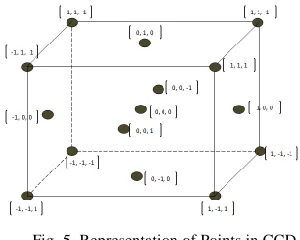
CCD is one of the most familiar experimental design of RSM. A central composite design contains three groups of design points such as factorial points, star or axial points and center points. Central composite designs are intended to approximate the coefficients of a quadratic model. All points are described in term of coded values

Fig. 5. Representation of Points in CCD

Factorial Points

In three level design, all levels of the considered factors are represented with -1, 0, 1. The 3-level factorial part of the design consists of all possible combinations of the -1, 0 and 1 levels of the factors. There are 8 design points possibility for three factor case in CCD as shown in figure 5.

(1, 1, 1) (1, 1, 1) (1, 1, 1) (1, 1, 1) (1, 1, 1) (1, 1, 1) (1, -1, 1) (--1, --1, 1)

Star or Axial Points

is also called as face-centered central composite design. By setting the alpha value equal to 1 or by selecting the points which are face centered. Position for the star points is at the face of the cube portion on the design. This design only requires three levels for each factor. The various possible combinations in this design are shown below

(-1, 0, 0) (1, 0, 0) (0, 0, -1) (0, 0, 1) (0, -1, 0) (0, 1, 0) Center Points

As the name indicates center points are the points with all level set to 0 that is midpoint of each factor: (0, 0, 0). By repeating center points for four to six times, it is possible to estimate the experimental error also called as pure error. To summarize CCD, require three levels of all factors and coded -1, 0, 1. The main characteristic of CCD is that its structure lends itself to chronological experimentation. CCD can be carried out in blocks.

4. RESULTS&DISCUSSION

After the completion of distinctive experiments, the bulge ratio and thinning ratio are calculated as per the equations and are shown in table 6.

Table VI Experimental outcomes

S.N

Internal Pressure (x1)

Axial Force (x2)

Length (x3) df/di (to-tf)/to

1 230 0.2 195 1.4326 0.1035

2 230 0.35 210 1.0182 0.1342

3 230 0.5 225 0.1225 0.3171

4 250 0.2 210 1.4542 0.1242

5 250 0.35 225 1.0046 0.2392

6 250 0.5 195 1.2135 0.2285

7 270 0.2 225 1.4389 0.125

8 270 0.35 195 1.4497 0.1095

9 270 0.5 210 1.1254 0.2925

4.1. Development of Empirical models

After completion of the experiments, the experimental data is collected which is relevant to output responses such as bulge ratio and thinning ratio and are used to employ the projected methodology.

The main objective of generating the numerical relationship between output responses to the input variables is to optimize THFP.

Design Expert 10 V is a statistical analysis tool [15], and is utilized to compute the regression coefficients of the proposed models.

4.2 Analysis of variance (ANOVA)

Analysis of variance (ANOVA) is carried out for the 2F1 response surface models. The statistical data of ANOVA for bulge ratio and thinning ratio are mentioned in the tables 7 and 8 respectively. Normally, if value of “Prob. > F” is less than 0.05, then that model is treated as significant. From the tables 7 and 8, it is noted that “Prob. > F” value are less than

0.05 in all instances for the given models, which indicates that the models [16] are significant and the following equations are obtained

(5)

Table VII

ANOVA [Partial sum of squares] for Df/Di

Source Sum of

Squares d. f.

Mean

Square F-Value Prob > F

Model 1.44 6 0.24 738.33 0.0014*

A-Internal pressure

0.036 1 0.036 110.82 0.0089

B-Axial

Force 0.28 1 0.28 863.10 0.0012

C-Length 0.061 1 0.061 188.31 0.0053

AB 0.049 1 0.049 149.34 0.0066

AC

1.278E-003 1

1.278E-003 3.92 0.1861

BC 0.070 1 0.070 216.21 0.0046

Residual

6.515E-004 2

3.257E-004 Core

Total 1.44 8

Std.

Dev. 0.018

R-Squared 0.9995

Mean 1.14 Adj

R-Squared 0.9982 * - Refers to Significant terms

4.3 Tests for Adequacy

The developed empirical models are tested for their adequacy using the following tests:

Multiple regression coefficients

Regression coefficient (R2) is computed to verify whether the fitted models actually describe the experimental data. R2 is used to deliberate the quality of the fit [16], and is defined as ratio between variability given by the model and total variability in the experimental data. If R2 is closer to 1, then the developed model fits to the experimental data. It is the proportion of variation in the dependent variable (response) that can be explained by the predictors (factor) in the model.

explain the variation in bulge ratio up to the extent of 99.95%. Similarly, from Table 8, it is found that R2 for thinning ratio is 0.9887. This shows that the 2nd –order model can explain the variation in thinning ratio up to the extent of 98.87%.

The adjusted R2 gives the possibility to get a more suitable value to estimate R2. The adjusted R2 value is calculated from the following expression

Adjusted R2= ₁ [(1 2)( 1)]

[ 1]

R N

N K

 



  (8)

Here, number of observations and number of predictors are denoted by N and K respectively. When N is small and K is large, it leads to large difference between R2 and adjusted R2 (since (N-1) / (N-K-1) << 1). Similarly, when N is very large and K is small, it leads to the value of R2 is much closer to adjusted R2 value (since (N-1) / (N-K-1) is closer to 1).From Table 7 and 8, it is found that the values of adjusted R2 of bulge ratio and thinning ratios 0.9982 and 0.9549 respectively.

From the ANOVA statistics, it is found that R2 and adjusted R2 values are closer to each other. This illustrate that the model which is developed can represent the process adequately.

Table VIII

ANOVA [Partial sum of squares] for (Ti-Tf)/Ti

Source

Sum of Squares d. f.

Mean

Square F-Value Prob > F

Model 0.069 6 0.012 29.26 0.0334*

A-Internal pressure

9.507E-003 1

9.507E-003 24.11 0.0391

B-Axial

Force 0.029 1 0.029 72.28 0.0136

C-Length

2.960E-003 1

2.960E-003 7.51 0.1114

AB

8.090E-003 1

8.090E-003 20.52 0.0454

AC 0.016 1 0.016 40.57 0.0238

BC

4.079E-003 1

4.079E-003 10.34 0.0846

Residual

7.886E-004 2

3.943E-004

Cor Total 0.070 8

Std. Dev. 0.020

R-Squared 0.9887

Mean 0.21 Adj

R-Squared 0.9549 * - Refers to Significant terms

Further, the adequacy of the developed model is verified for normal probability plot of residuals. The analytical graphs are drawn to verify where the data is normally distributed and for any assumption is violated. Thus the normal probability plots of residuals for bulge ratio and thinning ratio are plotted. These plots are useful for assessing the data whether data come from the normal distribution or not.

It is assumed that the normality is feasible when the data points are distributed nearer to the line in normal probability plot. If not, the points are spattered away from the line; the assumption of normality is treated as not feasible.

The normal probability plots of the residuals for bulge ratio and thinning ratio are shown in Fig.6 & Fig.7 respectively.

Fig. 6. Normal probability plot of residuals for df/di

Fig. 7. Normal probability plot of residuals for (to-tf)/to

From Fig.6 and Fig.7, it can be observed that, all residuals (data points) are scattered closer to the straight line, which means that the errors are distributed normally. Hence the developed empirical models are significant. Therefore these are used for optimization of process parameters.

5. CONCLUSIONS

parameter such as optimum internal pressure, axial feed and length of the tube for obtaining the desired product quality. The present investigation is mainly concentrated to develop the second-order polynomial models for the input process parameters by using the experimental data.

The R2 values for output responses are found to be 0.9995 and 0.9887 which are very close to unity indicates that the models can be used for further analysis and optimization. The normal plots are also plotted between the input factors and the output responses. Hence the tube hydro forming process can be automated by using this proposed methodology.

REFERENCES

[1] Ahmetoglu e Altan, 2000, Ahmetoglou, M., Altan, T., " Tube hydroforming: state-of-the-art and future trends ", Journal of Materials Processing Technology, vol. 98, 25-33, 2000.

[2] An Honggang, D.E. Green, J. Johrendt, (2010), Multi-objective optimization and sensitivity analysis of tube hydroforming simulations, Int.J. Advanced, Manufacturing Technology, DOI: 10.1007/s00170-009-2505-x

[3] Carleer B, Kevie G, Winter L, Veldhuizen B (2000) Analysis of the effect of material properties on the hydroforming process of tubes. J Mater Process Technol 104:158–166

[4] Boudeau N, Lejeune A, Gelin JC (2002) Influence of material and process parameters on the development of necking and bursting in flange and tube hydroforming. J Mater Process Technol 125–126:849–855

[5] Ko M, Altan T (2002) Application of two dimensional (2D) FEA for the tube hydroforming process. Int J Mach Tool Manuf 42:1285–1295

[6] Yang J, Jeon B, Oh S (2001) Design sensitivity analysis and Optimization of the hydroforming process. J Mater Process Technol 113:666–672

[7] Park K, Kim Y (1995) The effect of material and process variables on the stamping formability of sheet materials. J Mater Process Technol 51:64–78

[8] Lee SW (2002) Study on the forming parameters of the metal bellows. J Mater Process Technol 130–131:47–53

[9] Ko D, Kim D, Kim B (1999) Application of artificial neural network and Taguchi method to preform design in metal forming considering workability. Int J Mach Tool & Manuf 39:771–785

[10]Yang HJ, Hwang PJ, Lee SH (2002) A study on shrinkage compensation of the SLS process by using the Taguchi method. Int J Mach Tool Manu 42:1203-1212

[11]Jae-Seob Kwak., “Application of Taguchi and response surface methodologies for geometric error in surface grinding process”, Int J of machine Tools & Manufacturing, 45:327–334, 2005.

[12]Box G.E.P., Draper N.R., “Empirical model-building and response surfaces”, New York: John Wiley & Sons, 1987

[13]Myers R.H., Montgomery D.C., “Response surface methodology”, Wiley, New York, 1995.

[14]Montgomery D.C., “Design and analysis of experiments”, 5th edition, John Wiley & Sons, INC, New York, 2003.

[15]Design Expert, 7.1.3v, Stat-Ease Inc., 2021 E. Hennepin Avenue, Suite 480, Minneapolis, 2006.

[16]Myers R.H., Montgomery D.C., “Response surface methodology”, Wiley, New York, 1995.

ACKNOWLEDGEMENT