Fuzzy Logic Controller for Enhancement of Transient Stability in Multi Machine AC-DC Power Systems

(1)

IACSIT International Journal of Engineering and Technology, Vol.2, No.5, October 2010 ISSN: 1793-8236

423 Abstract—This paper discusses the impact of HVDC on Power System Stability and proposes a new control mechanism based on Fuzzy set theory to augment dynamic performance of a multi-machine power system. To have good damping characteristics over a wide range of operating conditions, deviations in speed and acceleration of the machines are chosen as the input signals to the fuzzy controller. These input signals are first characterized by a set of linguistic variables using fuzzy set notations .The fuzzy relation matrix allows a set of fuzzy logic operations that are performed on controller inputs to obtain the desired output. The effectiveness of the proposed controller is demonstrated by a multi-machine system example. The performance of this fuzzy controller, in comparison to the conventional fixed gain controller, demonstrates the efficacy of this new fuzzy PID controller.

Index Terms—HVDC, Eliminated variable method, Power System Stability, Multi–Machine Stability, Current controller, Fuzzy Logic Controller

I. INTRODUCTION

The choice between transmission alternatives is made on the basis of cost and controllability. The original justification for HVDC systems was its lower cost for long electrical distances, which, in the case of submarine (or underground) cable schemes, applies to relatively short geometrical distances. At present, the controllability factor justifies the DC alternative regardless of cost as evidenced by the growing number of back-to-back links in existence. HVDC systems have the ability to rapidly control the transmitted power. Therefore, they have a significant impact on the stability of the associated AC Power Systems. More importantly, proper design of the HVDC controls is essential to ensure satisfactory performance of overall AC/DC system [1].In recent years, the HVDC system models used are simpler models; such models are adequate for general purpose stability studies of systems in which the DC link is connected to stronger parts of the AC system. But the preference is to have a flexible modeling capability with a

Manuscript received July 27, 2010.

M.Uma Vani is with the Lakireddy Balireddy College of Engineering, Mylavaram, Andhra Pradesh, India (corresponding author, phone: 08659-222629; fax: 08659-222931; e-mail:[email protected]).

P.V.Ramana Rao is with the National Institute of Technology,Warangal, Andhra Pradesh, India (e-mail:[email protected]).

S.V.Jayaram Kumar is with the Jawaharlal Nehru Technological University, Hyderabad, Andhra Pradesh, India(e-mail: [email protected]).

required range of detail [2].

Supplementary controls are often required to exploit the controllability of DC links for enhancing the AC system dynamic performance. There are a variety of such higher level controls used in practice. Their performance objectives vary depending on the characteristics of the associated AC systems. The controls used tend to be unique to each system. To date, no attempt has been made to develop generalized control schemes applicable to all systems.

The supplementary controls use signals derived from the AC systems to modulate the DC quantities.

Some of the conventional controls that can be used are as follows:

• Rotor frequency of adjacent generator • Frequency at the converter bus

• Power or current in adjacent, parallel AC tie. • Phase angle changes in the AC system [3].

The above signals work satisfactorily for the single machine system case. However, in the case of multi machine system it may be necessary to employ control signals derived from relative angle deviation, speed deviation and acceleration and different combinations of these signals. Apart from linear controllers (like P, PI and PID controllers), adaptive controllers can also be employed which are known to give better performance. The particular choice depends on the system characteristics and the desired results.

Numerous modern control techniques are reported in literature and already used in several ac-dc systems for deriving the necessary modulation signals to respective control schemes [4]-[7]. Most of these techniques need accurate mathematical models of the system under consideration for designing the controller. However, the highly complex and non-linear nature of power systems causes the derivation of accurate models extremely difficult. Therefore, there exist some limitations for the mathematical model based schemes. In order to overcome these limitations, applications of new intelligent technologies such as fuzzy systems, neural networks, and genetic algorithms have been investigated in different areas of power systems for reliable and high quality power supply at low cost.

Design of a fuzzy logic controller does not need an accurate mathematical model of the system under consideration. A qualitative knowledge about the system behavior is adequate to design a fuzzy logic controller to achieve a desired control objective. In addition, it is easy to

Uma Vani Marreddy , Ramana Rao P.V. and Jayaram Kumar S.V.

Fuzzy Logic Controller for Enhancement of

Transient Stability in Multi Machine AC-DC

(2)

424 fuzzy logic controller is not significantly affected due to changes in system operating conditions and parameters.

The output of Fuzzy Logic Controller can be utilized to modulate the power order of the DC control, which in turn modulates the DC power. The stabilizing control is implemented through large signal modulation of power in response to a control signal derived from the AC system variables. The effectiveness of the control can be enhanced by increased overload rating of the converters which permit short – term overloads.

In this paper, apart from conventional controller, a fuzzy logic based controller is developed to modulate the power order of the DC control, which in turn modulates the DC power.、

II. AC/DCSTABILITY ANALYSIS

In transient stability studies, it is prerequisite to do AC/DC load flow calculations in order to obtain system conditions prior to the disturbance. The eliminated variable method proposed in [8] is used here, which treats the real and reactive powers consumed by the converters as voltage dependent loads. The DC equations are solved analytically or numerically and the DC variables are eliminated from the power flow equations. The method is unified, since the effect of the DC-link is included in the Jacobian. It is, however, not an extended variable method, since no DC variables are added to the solution vector.

A. DC system model

The equations describing the steady state behavior of a mono polar DC link of Fig 1 can be summarized as follows.

V_dr 3 2 a V_{r tr} cosα_r 3 X I_c _d

π π

= − (1)

3 2 3 cos V_di a V_{i ti} γ_i X I_c _d π π = − (2)

V_dr =V_di +r I_{d d} (3)

P_dr =V_{dr d}I (4)

P_di =V_{di d}I (5)

3 2 S_dr k a V I_{r tr} _d π = (6)

3 2 S_di k a V I_{i ti} _d π = (7)

2 2 Q_dr = S_dr −P_dr (8)

2 2 Q_di = S_di −P_di (9)

where k is assumed constant, k≈0.995.See Appendix-II. Fig. 1:Model of DC converter are written asfunctions of Vtr and Vti. The expressions for their partial derivatives with respect to Vtr and Vti [8] are computed and used in modification of Jacobian elements of the Newton Raphson power flow as shown below:

/

H

N

P

J

L

Q

V V

δ

⎡

⎤

Δ

⎡

⎤

⎡

⎤

= ⎢

⎥

⎢

_Δ

⎥

⎢

_Δ

⎥

⎣

⎦

⎣

⎦

⎣

Each DC system tends to have unique characteristics tailored to meet the specific needs of its application. Therefore, standard models of fixed structures have not been developed for representation of DC systems in stability studies. The current controller employed here (Fig 2) is a proportional integral controller and the auxiliary controller is taken to be a constant gain controller.

Fig. 2: Current controller and auxiliary controller

HVDC line is represented using transfer function model [9] as shown in the Fig 3.

Fig. 3: Transfer function model

In this case, the time constant of the DC link [9] Tdc (=

Ldc/Rdc))represents the delay in establishing the DC current

after a step change in the current order is given.

D. Generator Representation

(3)

425 speed, a normal and accepted assumption for stability studies, then M is constant. If the rotational power losses of the machine due to such effects as windage and friction are ignored, then the accelerating power equals the difference between the mechanical power and the electrical power [10]. The classical model can be described by the following set of differential and algebraic equations:

Differential:

(

)

2

m e

d

f

dt

d

f

P

dt

H

δ ω π

δ

ω π

= −

=

−

(15)

Algebraic:

E

'

=

E

_t

+

r I

_{a t}

+

jx I

_{d t}' (16)

Where, E′=voltage behind transient reactance Et=machine terminal voltage

It=machine terminal current

ra=armature resistance

x

_d' =transient reactance

Fig. 4: Generator Classical model

E. Representation of Loads

The static admittance Ypo used to represent the load at

bus-p, can be obtained from

_po po

p

I

Y

E

=

where, _po lp _* lp

p

P

jQ

I

E

−

=

(17)

where Ep is the calculated bus voltage, Plp and Qlp are the

scheduled bus loads. Diagonal elements of admittance matrix (Y–Bus) corresponding to the load bus are modified using the Ypo.

F. Steps of the AC-DC Transient Stability Study

Generally, the DC scheme interconnects two or more, otherwise independent, AC systems and the stability assessment is carried out for each of them separately, taking into account the power constraints at the converter terminal. If the DC link is part of a single (synchronous) AC system, the converter constraints will apply to each of the nodes containing a converter terminal.

The basic structure of transient stability program [11] is given below :

1) The initial bus voltages are obtained from the AC/DC load flow solution prior to the disturbance. 2) After the AC/DC load flow solution is obtained, the

machine currents and voltages behind transient reactance are calculated.

3) The initial speed is equated to 2

π

f and the initial mechanical power is equated to the real power output of each machine prior to the disturbance. 4) The network data is modified for the new

representation. Extra nodes are added to represent

the generator internal voltages. Admittance matrix is modified to incorporate the load representation. 5) Set time, t=0.

6) If there is any switching operation or change in fault condition, modify network data accordingly and run the AC/DC load flow.

7) Using Runge-Kutta method, solve the machine differential equations to find the changes in the internal voltage angle and machine speeds.

8) Internal voltage angles and machine speeds are updated and are stored for plotting.

9) AC/DC load flow is run to get the new output powers of the machine.

10) Advance time, t=t+Δt.

11) Check for time limit, if t ≤ tmax repeat the process from step 6, else plot the graphs of internal voltage angle variations and stop the process.

Basing on the plots, that we get from the above procedure it can be decided whether the system is stable or unstable. In case of multi machine system stability analysis the plot of relative angles is done to evaluate the stability.

III. CONVENTIONAL CONTROLLER

The WSCC 3-Machine, 9-Bus system [10] is considered for the stability analysis and is given in Fig 5.

Fig. 5: WSCC three-machine, nine-bus system

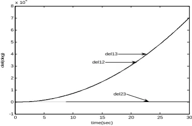
A HVDC line is assumed to be present between buses 4–5. A three phase to ground fault is assumed to occur on the line 4 – 6, near bus-6, at initial time zero. It is cleared after 4 cycles, by removing the line and to reflect this removal the admittance matrix is modified. Initially, HVDC line is assumed to maintain same control as it had in the normal condition. The power flowing through the HVDC link is maintained constant and equal to pre-fault value. Then the plot of relative angles is as shown in Fig 6.

0 5 10 15 20 25 30

-1 0 1 2 3 4 5 6 7 8x 10

4

time(sec)

de

l(

de

g) del13

del12

del23

(4)

426

0 5 10 15 20 25 30

-4 -3 -2 -1 0 1 2 3 4

time(sec)

del

(d

eg)

del1

del2 del3

Fig. 7: Plot of generator absolute angles without any control

From the Figs 6&7 it is clear that the system is unstable as the relative angles are increasing. It can be examined that the generator-1 is going out of step with respect to the generators 2 and 3. To stabilize the system it is necessary to make the accelerations of all the generators equal. So an error signal representing average difference in accelerations of the generators is considered. In case of multi-machine systems the relative angles are to be maintained within limits to maintain the stability of the system. So, error signals derived from the average difference in the relative angles and average difference in the relative speeds of the generators are considered. These error signals [2] are as shown below:

( ) ( )

(

)

(

( ) ( )

)

_{( ) ( )}

1

2 1 3 1

2 3

2

error=⎢⎡⎡⎢ ω −ω + ω −ω ⎤⎥ ⎣−⎡ω −ω ⎤_⎦⎤⎥

⎢⎢_⎣ ⎥_⎦ ⎥

⎣ ⎦

(18)

( )

(

)

(

( )

)

_{( )}

2

2 1 3 1

2 3

2

del del del del

error del del

⎡⎡ − + − ⎤⎤

=⎢⎢ _{⎥ ⎣}⎥−⎡ − ⎤_⎦

⎢⎢_⎣ ⎥_⎦⎥

⎣ ⎦

(19)

( )

( ) ( )( ) ( )

( )

3

_ 3 _ 2

3 2 _ 1

2 1

P mis P mis

H H P mis

error

H

⎡ ⎤

+

⎢ _{⎥ ⎡} _⎤

⎢ ⎥

=_⎢ _{⎥ ⎣}− ⎢ ⎥

⎦

⎢ ⎥

⎣ ⎦

(20) When all the three signals given by (18), (19) and (20)are considered, the plot of the relative angles is as shown in Fig 8. It can be seen that the stability of the system is improved and by the end of the study time the action of AGC will come into picture which will further improve the system stability.

0 5 10 15 20 25 30

-40 -20 0 20 40 60 80 100 120

Time(sec)

De

l(

d

e

g

)

del12

del23 del13

Fig. 8: Plot of relative angles with control signal Kp*error1+ Ki*error2+Kd*error3.

Control signal is given by the following expression:

error = Kp*error1+ Ki*error2 + Kd*error3 (21)

Here, the signal error2 is the equivalent to the integral of

the signal error1, and the signal error3 is equivalent to the

differential of the signal error1.Hence, the controller

proposed above is equivalent to a PID controller. Then the control signal can be equivalently represented as in (22).

error = Kp*e(t)+Ki*Ie(t)+Kd*De(t) (22)

IV. FUZZY LOGIC CONTROLLER

Here a fuzzy logic controller is used with the error1(∆ω)

and error3(∆ώ) [12] as its inputs and the resultant error of the

PID control scheme has been adopted as input for the purpose of enhancing the stability of multi-machine power systems, utilizing HVDC power modulation. In this scheme, the error signals error1 and error3 control signals, as specified in the

previous section, are fuzzified at every sampling interval, in accordance with a set of linguistic control rules and in conjunction with fuzzy logic. And output fuzzy value is defuzzified using min-max method. This feature is desirable because as the operating conditions of a system begin to change, deterioration in performance will result if a fixed gain controller is applied. Consequently, the proposed control scheme has the advantages of a conventional PID controller and that of a fuzzy logic controller.

A. Fuzzy Relation

Let A and B be two fuzzy sets with membership functions

µA(x)and µB(x), respectively. A fuzzy relation R from A to B

can be visualized as a fuzzy graph and can be characterized by the membership function µR(x,y) which satisfies the

composition rule as follows:

µB(y)=maxx(min(µR(x,y)µA(x))) (23)

In many cases it is convenient to express the membership function of a fuzzy subset of the real line in terms of a standard function whose parameters may be adjusted to fit a specified membership function in a suitable fashion.

B. Design of the Fuzzy Controller for Power System Stability

To determine the controller output from the measured system variables error1 and error3, a fuzzy relation matrix R,

which gives the relationship between the fuzzy set characterizing inputs and the fuzzy set characterizer output, is computed as follows:

Step 1: Use membership functions to represent controller inputs error3 and error1 in fuzzy set notation.

Step 2: Use the composition rule in (23) to determine the membership function of the resultant error output.

Step 3: Determine a proper resultant error output from the membership function of the output signal.

(5)

427 following discussions.

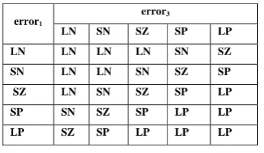
C. Establishment of the Fuzzy Relation Matrix

A fuzzy relation matrix must be set up and stored in computer memory. A set of decision rules relating inputs to the output are first compiled. These decision rules are expressed using linguistic variables such as large positive (LP), medium positive (MP), small positive (SP), very small (VS), small negative (SN), medium negative (MN), and large negative (LN).

For example, a typical rule reads as follows:

Rule-1: If error1 is LP and error3 is LN, then errorres should

be VS. (24)

Fig. 9: Membership function for 7 variables

Through the combination of the two input signals error3

and error1, there will be 49 decision rules in all. The most

convenient way to present these decision rules is to use a decision table as shown in Table-I. It is observed from Table-I that each entry represents a particular rule.

TABLE I: DECISION TABLE FOR SEVEN MEMBERSHIP VARIABLES

error3

LN MN SN VS SP MP LP

LP VS SP MP LP LP LP LP

MP SN VS SP MP MP LP LP

SP MN SN VS SP SP MP LP

VS MN MN SN VS SP MP MP

SN LN MN SN SN VS SP MP

MN LN LN MN MN SN VS SP

LN LN LN LN LN MN SN VS

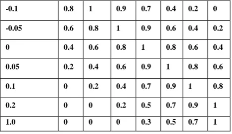
Using these normalized quantities, controller inputs can be described by membership functions for the linguistic variables, as shown in Table-II. Note that only the membership functions for nine different values of error3 and

error1 are given in Table-II. For a value of error3 or error1

which is not listed in Table-II, linear interpolation must be employed to determine the membership function.

TABLE II: MEMBERSHIP FUNCTIONS FOR INPUTS

Normalized

error1 and

error3

Membership functions

LN MN SN VS SP MP LP

-1.0 1 0.7 0.5 0.3 0 0 0

-0.2 1 0.9 0.7 0.5 0.2 0 0

-0.1 0.8 1 0.9 0.7 0.4 0.2 0

-0.05 0.6 0.8 1 0.9 0.6 0.4 0.2

0 0.4 0.6 0.8 1 0.8 0.6 0.4

0.05 0.2 0.4 0.6 0.9 1 0.8 0.6

0.1 0 0.2 0.4 0.7 0.9 1 0.8

0.2 0 0 0.2 0.5 0.7 0.9 1

1.0 0 0 0 0.3 0.5 0.7 1

Let us demonstrate the use of Table-II by an example. At a particular sampling instant, let the sampled controller inputs be, say error1 =0.2 and error3 = - 0.1. From Table-II, the two

controller inputs can be described by the following fuzzy sets:

error1:{(LN,0),(MN,0),(SN,0.2),(VS,0.5),(SP,0.7),

(MP,0.9),(LP,1)} (25)

error3:{(LN,0.8),(MN,1),(SN,0.9),(VS,0.7),(SP,0.4),

(MP,0.2),(LP,0)} (26)

D. Determination of the Resultant Error Output

Once the membership values for controller output have been computed, a suitable algorithm must be employed to determine the resultant error output signal. The algorithm adopted in this work is the ‘maximum algorithm’ in which the signal with largest membership value is chosen as the resultant error output signal. The resultant error output expressed in linguistic terms must be converted back to numerical values before it can be fed into the controller. The conversion table as shown in the Table-III has been compiled based on the controller signals obtained in the conventional controller design. A different set of numerical values can be selected and different dynamic responses will be obtained. The difference will however be insignificant since the error signal must be within the narrow range from -7.5 to 7. The table is stored in computer memory as a look-up table. It is observed from Table-III that the numerical value of the stabilizing signal for our example is 1.8.

TABLE III: CONVERSION TABLE FROM 7 LINGUISTIC VARIABLES TO NUMERICAL VALUES

errorres

LN MN SN VS SP MP LP

-7.5 -5 - 2.25 0.5 1.8 4.5 7

Similarly, the above fuzzy controller is implemented by using 5 membership functions, with the rule and conversion tables as shown in Tables: IV &V.

.

Fig. 10: Membership function with 5 fuzzy sets

(6)

428

LN LN LN LN SN SZ

SN LN LN SN SZ SP

SZ LN SN SZ SP LP

SP SN SZ SP LP LP

LP SZ SP LP LP LP

TABLE V: CONVERSION TABLE FROM 5 LINGUISTIC VARIABLES TO NUMERICAL VALUES

errorres

LN SN SZ SP LP

-8 -3 0.5 3 8

Figures: 11&12 denote the variation of relative rotor angles with seven, and five membership functions respectively.

0 5 10 15 20 25 30

-40 -20 0 20 40 60 80 100 120 140 160

time(sec)

de

l(

deg)

del13

del12

del23

Fig. 11: Plot of relative angles with proposed fuzzy logic controller (7 membership function)

0 5 10 15 20 25 30

-50 0 50 100 150 200

time(sec)

de

l(

deg)

K1=0.0006 K2=0.003

del 13 del 12

del 23

Fig. 12: Plot of relative angles with proposed fuzzy logic controller (5 membership function)

V. CONCLUSIONS

Considering the HVDC current controller and line dynamics, it is observed that the transient stability of the multi-machine system is improved when the combination of all the three signals derived from relative speed, phase angle and average acceleration is used.

The paper presents a new approach to the design of a supplementary stabilizing controller for an HVDC transmission link using fuzzy logic. Results from this work reveal that, under disturbance conditions, better dynamic performance can be achieved using the proposed fuzzy controller than a conventional supplementary controller. Further improved performance can be obtained by suitably

output feedback control law developed in this paper requires only local measurements within each generating unit.

Research is being carried out to design a Hybrid Neuro-Fuzzy supplementary controller for two-terminal HVDC-AC systems for improvement of multi machine transient stability.

APPENDIX I

DC Line Data

rd = 0.017pu , Xc = 0.6pu , Ld = 0.05pu

alfamin = 5º , alfamax = 80º

tapr,min = 0.96 , tapr,max = 1.06

tapi,min = 0.99 , tapi,max = 1.09

Initial Conditions

alfa = 0.2094c_{, I}

d=0.3691pu, Pdi=0.406pu

Vdi=1.1pu , gama=0.3142c, PM[1]=0.756646pu PM[2]=1.63pu,

PM[3]=0.85pu, δM[1]=2.388448º δM[2]=18.603189º , δM[3]=12.314856º

APPENDIX II

List of Symbols

Vd Direct voltage

Id Direct current

a Converter transformer tap ratio

α Firing angle u Overlap angle

γ Extinction angle

Pd Real power consumed by the converter

Qd Reactive power consumed by the converter

Sd Magnitude of complex power consumed by

converter and transformer PL = RdId2

QL= (3/Π) Xc Id2

k = (Iac/Id)*(Π/3√2) , k≈ 0.995 ka = k/cosα

kγ= k/cosγ

Xc Commutating reactance

Rd DC line resistance

V Vector of nodal voltage magnitudes

Θ Vector of nodal voltage angles

∆P Vector of real power mismatches

∆Q Vector of reactive power mismatches Ptspec Specified real power at converter terminal

Qtspec Specified reactive power at converter

terminal

Ptac Real power transmitted by the ac network Qtac Reactive power transmitted by the ac network

All quantities are given in p.u. Subscript t refers to the converter ac terminals. Subscript r refers to the rectifier and i to the inverter.

REFERENCES

[1] Prabha Kundur, “Power System Stability and Control”, McGraw- Hill, Inc., 1994.

(7)

429

[3] “IEEE Guide for Planning DC Links Terminating at AC Locations Having Low Short-Circuit Capacities”, The Institute of Electrical and Electronics Engineers, Inc., 1997.

[4] Y.Y. Hsu, and L. Wang, “Damping of a parallel ac-dc power system using PID power system stabilisers and rectifier current regulators”, IEEE Trans. Energy Conversion, vol. 3, no. 3, September 1988, pp. 540-547.

[5] A.S. Emarah, M.A. Choudhry, and G.D. Galanos, “Design of Optimal Modulation Controllers for Multi- area AC/DC Systems using eigen value sensitivities”, IEEE Trans. Power System, vol. PWRS-2, no. 3, August 1987, pp. 522-528.

[6] P.K. Dash, A.C. Liew, and A. Routray, “High performance Controllers for HVDC Transmission Links”, IEE Proc.-Gener.Transm.Distrib., vol. 141, no. 5, September 1994, pp. 422-428.

[7] K.W.V. To, A.K. David, and A.F. Hammad, “A robust coordinated control scheme for HVDC transmission with parallel ac systems”, IEEE Trans. Power Delivery, vol. 9, no. 3, July 1994, pp. 1710-1716. [8] T. Smed, G. Anderson, G.B.Sheble, L.L.Grisby “A New Approach to

AC/DC Power Flow”,IEEE Trans. on Power Systems., Vol. 6, No. 3, pp1238- 1244, Aug.1991.

[9] K. R. Padiyar, “HVDC Power Transmission Systems”, New Age International (P) Ltd.,2004.

[10] P.M.Anderson and A.A.Fouad, “Power System Control and Stability”,1st_{ed.,Iowa State University Press,1977.}

[11] Stagg and El- Abiad, “Computer Methods in Power System Analysis”,International student Edition, McGraw- Hill, Book Company, 1968.

[12] Y.Y.Hsu & C.H.Cheng, “Design of fuzzy power system stabilizers for multi-machine power systems”,IEE Proceedings,vol.137,No.3,May 1990.

Uma Vani Marreddy received her B.Tech and M.Tech degrees from

V.R.Siddhartha Engineering College Vijayawada, A.P., India and NIT Warangal, A.P., India respectively, all in Electrical Engineering. Pursuing Ph.D from JNTU, Hyderabad, A.P., India. Currently, she is an Associate Professor in the Electrical and Electronics Engineering Department at Lakireddy Bali Reddy College of Engineering, Mylavaram, A.P., India and pursuing her Ph.D. from JNTU Hyderabad. Her major research interests include Power System Stability, AI techniques applications to Power System problems, HVDC controls and FACTS devices.

Ramana Rao P.V. born in 1946, India. Received his B.Tech., M.Tech., and

Ph.D degrees from IIT Madras, IIT Kharagpur and REC Warangal, India respectively, all in Electrical Engineering. Currently, he is a Professor in the Electrical Engineering Department at NIT Warangal , A.P., India. His major research interests include Power System Protection and Stability, HVDC controls , FACTS devices , Artificial Intelligence & Wavelet techniques applications to Power Systems.

S.V. Jayaram Kumar received his M.E. degree in power systems in 1979