Computational Fluid Dynamics Simulation of the Flow Field of Direct Methanol Fuel Cells

Computational Fluid Dynamics Simulation of the

Flow Field of Direct Methanol Fuel Cells

N. H. Maslan

, M. I. Rosli

, C. W. Goh

, M. S. Masdar

1

Fuel Cell Institute, Universiti Kebangsaan Malaysia, 43600 UKM Bangi, Selangor, Malaysia

2 _{Department of Chemical and Process Engineering, Faculty of Engineering and Built Environment, Universiti Kebangsaan}

Malaysia, 43600 UKM Bangi, Selangor, Malaysia *Corresponding author: [email protected]

Abstract--

Index Term-- Direct methanol fuel cell (DMFC); flow field; methanol mole fraction; velocity; pressure

1. INTRODUCTION

In a direct methanol fuel cell (DMFC), the anode flow field has two functions. The first function is to provide a channel for methanol to flow on the membrane electrode assembly (MEA) surface. Continuous supply of methanol to cell and uniform methanol distribution on the MEA surface are important for DMFC efficiency [1]. The design of flow field plays an important role in meeting both of these requirements. The second function is to provide a passage for the removal of CO2 produced from the reaction [2]. The efficient removal of

CO2 is essential in DMFC design [3]. A number of studies

demonstrated that the geometry of the flow field affects the mass transport of methanol to the diffusion layer and DMFC performance [1, 4-6]. CO2 gas bubbles and pressure drop are

also affected by the geometry of the flow field. Thus, optimizing the anode flow field is significant to achieve an optimal design of DMFC. In this study, five different flow field geometries, namely, a zigzag flow, a parallel flow, and three different serpentine flows with different flow channels, were investigated.

Computational fluid dynamics (CFD) is a fluid mechanic branch that uses numerical methods and algorithms to solve and analyze problems related to fluid flow [7]. CFD is used in fuel cell development to investigate the physical and chemical processes that occur in a fuel cell numerically, particularly the efficiency of multi-component transport in reactants and oxidants and its effects on the electrochemistry kinetics and performance of a fuel cell. CFD analysis can provide the performance characteristic of fuel cells under various operating conditions, catalysts, and membranes, among others. This analysis reduces the development cost by reducing the operating cost.

This study focused on the CFD simulation development of DMFC by using ESI CFD-ACE+ software. The flow field design that can optimize DMFC performance was determined based on the distributions of velocity, pressure, and methanol concentration in DMFC. The flow field patterns used were serpentine, zigzag, and parallel. The effects of anode channel width on DMFC performance were also investigated to determine its optimal performance. The widths of serpentine flow field channels used were 1.0, 1.5, and 2.0 mm. CFD simulations of DMFC were conducted using ESI CFD-ACE+ software to describe and analyze the flow pattern distributions of velocity, pressure, and methanol mole fraction by changing the anode flow field patterns and channel widths.

2. METHODOLOGY

CFD simulation in DMFC was developed by conducting three main steps, namely, pre-processing using CFD-GEOM, solutions and calculations using CFD-ACE-GUI, and post-processing using CFD-VIEW.

2.1. Pre-processing: CFD-GEOM software

NOMENCLATURE Abbreviations

J Current density, A m-2 CFD Computational fluid dynamics

J0 Reference exchange current density, A m

-3

DMFC Direct methanol fuel cell

p Pressure, Pa IGL Ideal gas law

S/V Surface to volume ratio, m2 m3 MEA Membrane electrode assembly

T Temperature, K MKT Mixed kinetic theory

Greek letters MOR Methanol oxidation reaction

α Transfer coefficient ORR Oxygen reduction reaction

Γ Mass diffusivity, kg m-1s-1 PFF Parallel flow field

γ Concentration parameter Sc Schmidt number

ɛ Porosity SSFF Serpentine flow field

κ Permeability, m2 Zigzag Zigzag flow field

μ Viscosity, kg m-1s-1 Subscripts

ρ Density, kg m-3 a Anode side of the membrane

σ Electrical conductivity, Ω-1

m-1 c Cathode side of the membrane

τ Bruggeman factor CH3OH Methanol

O2 Oxygen

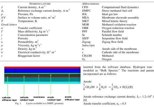
Fig. 1. Layers available in a DMFC geometry

Table II shows the depth of each layer. All five DMFC geometries were created. A triangular mesh was used for mesh generation (meshing). The dimension of each geometry was 40 mm × 40 mm. The operating parameters used are shown in Table III.

2.2. Solution and calculation: CFD-ACE-GUI software

After DMFC geometry was created, CFD-ACE-GUI was used to complete the calculation based on operating conditions and the reaction of chemical species in DMFC. Flow, chemistry, and electric modules were activated in CFD-ACE-GUI software to begin the calculation based on the selected modules. The chemical species available in DMFC were

inserted from the software database. Hydrogen ions were modeled as “Bulk Species.” The reactions and parameters incorporated are as follows.

Anode:

(1)

Anode reference exchange current density, J0 = 1.2×106 A m-3

[8]

Anode transfer coefficient, αa = 0.5 [8]

Cathode:

(2)

Cathode reference exchange current density, J0 = 1407 A m-3[8]

Cathode transfer coefficient, αc = 1.55

The parameter settings for each volume, porous medium volume, boundary, and initial conditions are shown in Tables IV, V, VI, and VII, respectively. When all parameters were set, the simulation was run using CFD-ACE-GUI.

Table I

Geometry dimensions of selected anode flow fields

Flow Field SSFF1 SSFF2 SSFF3 PFF Zigzag

Channel width (mm) _{2.00 1.50 1.00 2.00 1.50}

Channel depth (mm) _{2.00 2.00 2.00 2.00 2.00}

Cross section area (mm2) _{4.00 3.00 2.00 4.00 3.00}

Channel length (mm) _{425.00 569.00 843.40 422.40 562.50}

Value of exposed channel to

membrane area (mm2) 850.00 858.00 847.40 844.80 851.25

Table II

List of thickness for each layers [8]

Layer Thickness (mm)

Anode currentcollector 0.500

Anode channel 2.000

Anode diffusion layer 0.190

Anode catalyst layer 0.030

Membrane 0.127

Cathode catalyst layer 0.030

Cathode diffusion layer 0.190

Cathode channel 2.000

Cathode current collector 0.500

Table III

Operating parameter used in DMFC [1]

Operating parameter Value

Methanol concentration 1 M

Operating temperature 333 K

Active area dimension 4.0×4.0 cm Methanol inlet flow rate 2.0 ml min-1

2.3. Post-processing: CFD-VIEW software

In the last stage, CFD-VIEW was used to visualize and analyze CFD images. The distributions of velocity, pressure, and methanol mole fraction in the anode channel were determined.

Table IV

List of parameter setting for each volume conditions [9, 10]

Volume Name ρ (kg/m3) μ (kg/m.s) σ (Ω-1 m-1) Γ (kgm-1s-1)

Anode catalyst layer IGL MKT 4.2 Sc = 0.7

Anode channel 960 3.49×10-4 1.0×10-20 Sc = 0.7

Anode collector 2698.9 - 3703 -

Anode diffusion layer IGL MKT 1.0×10-20 Sc = 0.7

Cathode catalyst layer IGL MKT 1.0×10-20 Sc = 0.7

Cathode channel IGL MKT 1.0×10-20 Sc = 0.7

Cathode collector 2698.9 - 3703 -

Cathode diffusion layer IGL MKT 1.0×10-20 Sc = 0.7

Membrane IGL MKT Membrane model Sc = 0.7

Table V

List of porous media setting for each volume condition [9, 11]

Volume Name ε κ Reaction S/V Pore Diffusivity σ

Anode catalyst layer 0.3 1.0×10-14 MOR 1000 1.5×10-6 Bruggeman (1.5) 53

Anode diffusion layer 0.7 2.0×10-12 - - 1.0×10-6 Bruggeman (1.5) 53

Cathode catalyst layer 0.3 1.0×10-14 ORR 1000 1.5×10-6 Bruggeman (1.5) 53

Cathode diffusion layer 0.7 2.0×10-12 - - 1.0×10-6 Bruggeman (1.5) 53

Membrane 0.3 2.0×10-18 - - 1.0×10-6 Bruggeman (5) 0.7

Table VI

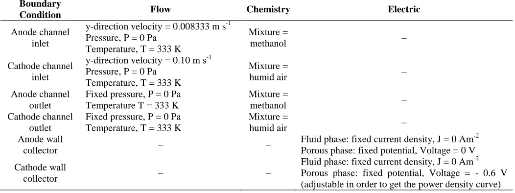
List of parameter setting for boundary conditions

Boundary

Condition Flow Chemistry Electric

Anode channel inlet

y-direction velocity = 0.008333 m s-1 Pressure, P = 0 Pa

Temperature, T = 333 K

Mixture =

methanol –

Cathode channel inlet

y-direction velocity = 0.10 m s-1 Pressure, P = 0 Pa

Temperature, T = 333 K

Mixture =

humid air –

Anode channel outlet

Fixed pressure, P = 0 Pa Temperature T = 333 K

Mixture =

methanol –

Cathode channel outlet

Fixed pressure, P = 0 Pa Temperature, T = 333 K

Mixture =

humid air –

Anode wall

collector – –

Fluid phase: fixed current density, J = 0 Am-2 Porous phase: fixed potential, Voltage = 0 V Cathode wall

collector – –

Table VII

List of parameter setting for initial conditions

Initial Volume

Conditions Flow Chemistry Heat

Anode catalyst layer Pressure = 90 000 Pa Mixture = humid air Temperature = 333 K

Cathode channel Pressure = 90 000 Pa Mixture = humid air Temperature = 333 K

Anode channnel – Mixture = methanol Temperature = 333 K

Anode catalyst layer – Mixture = nitrogen Temperature = 333 K

Anode diffusion layer – Mixture = nitrogen Temperature = 333 K

Cathode diffusion layer – Mixture = nitrogen Temperature = 333 K

Membrane – Mixture = nitrogen Temperature = 333 K

3. RESULTS AND DISCUSSION

3.1 Comparisons of power density curve between

experiment and simulation

The power density curve was plotted for comparison by using the simulation data of single-serpentine flow field (SSFF) 1 geometry and the experimental data by Yang and Zhao [1] (Figure 2). The simulation results and experimental data in Figure 2 present the same patterns in power density curve from cell voltages of 0 V to 0.5 V. According to Yang and Zhao [1], DMFC has a maximum power density of 54 mW cm−2 at a cell voltage of 0.27 V. In SSFF1 simulation, a maximum power density of 45 mW cm−2 was reached at a cell voltage of 0.55 V. The maximum power density difference was 9 mW cm−2. The simulation results were not 100% consistent with the experimental data. However, Figure 2 shows that the simulation results are similar to the experimental data in a fuel cell operating at low cell voltages from 0 to 0.5 V. Therefore, the DMFCs operated at a cell voltage of 0.261 V were used to visualize the velocity, pressure, and methanol mole fraction distributions in CFD. The same parameters were used in all simulated geometries.

Fig. 2. Comparison between simulation and experiment of SSFF1

3.2 Effects of anode flow field design on DMFC

performance

In this study, three different flow fields with the same open ratio, that is, 53%, were simulated at a voltage cell of 0.261 V to investigate the velocity, pressure, and methanol mole fraction distributions by using CFD.

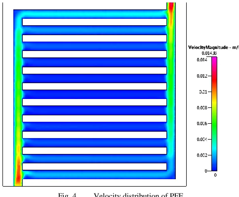
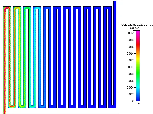
3.2.1 Velocity distribution of different flow fields

Figures 3, 4 and 5 show that the velocity distribution of SSFF1 was uniform and had a high magnitude along the channel while at PFF showed highly non-uniform velocity distribution. These conditions at SSFF1 benefit the removal of produced CO2 and increase the mass transport of methanol from the

flow channel to the diffusion layer [4], which increases DMFC performance. Meanwhile, the velocity in PFF shows a stagnant zone in the central regions but high values at lateral channels [3]. This affects the collected CO2 gas in the PFF

anode channel. Thus, the effective contact area between methanol and the diffusion layer becomes small [1]. The flow velocity of PFF decreases drastically and differs in each channel because of the free excess methanol. This phenomenon affects DMFC performance. The zigzag flow field is a combination of serpentine flow field and PFF. The results obtained were similar to PFF because the velocity distribution was not uniform in the zigzag flow field.

Fig. 4. Velocity distribution of PFF Fig. 5. Velocity distribution of zigzag

3.2.2 Pressure distribution of different flow fields

Figures 6, 7, and 8 present the pressure distributions of SSFF1, PFF and zigzag flow field, respectively. The SSFF1 design showed a uniform pressure distribution. SSFF1 exhibited the highest pressure drop (7.506 Pa). The pressure drop values for the zigzag flow field and PFF were 1.554 and 0.4961 Pa, respectively. These results show that PFF is only 1/15 of SSFF1. SSFF1 and zigzag flow fields require high pressure drop but not the PFF [12]. SSFF1 is expected to have a better

DMFC performance because its higher pressure drop contributes to increased efficiency of methanol transport. Hence, the removal of CO2 gas becomes easier. Its higher

pressure drop also contributes to a uniform fluid velocity distribution, which leads to increased DMFC performance. The pressure drop in the zigzag flow field was higher than that in PFF; thus, the former is expected to perform better than the latter.

Fig. 8. Pressure distribution of zigzag

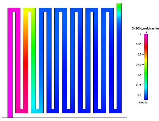
3.2.3 Methanol mole fraction distribution

The methanol mole fraction distribution along the channel is given in Figures 9, 10 and 11. As shown in Figures 9, the methanol mole fraction at SSFF1 decreased from 1 to 0.864 at the anode channel outlet, whereas that along the PFF channel was considered high because it decreased from 1 to 0.9281

only (Figure 10). Hence, only a small amount of methanol reacted to generate electricity. The zigzag flow field exhibited the highest drop of methanol mole fraction, which is from 1 to 0.6518. This result may be due to the methanol crossover. The methanol concentration is declined along the channel due to the electrochemical reaction [3].

Fig. 11. Methanol mole fraction distribution of zigzag

3.2.4 Comparisons of SSFF1, PFF and zigzag flow field

Based on the comparisons of the velocity, pressure, and methanol mole fraction distributions in SSFF1, PFF, and zigzag flow field, SSFF1 showed the most uniform velocity distribution, the highest pressure drop, and the most uniform methanol mole fraction distribution. Thus, SSFF1 is assumed to have the highest DMFC performance. The power densities simulated from all flow fields are shown in Figure 12. SSFF1 had the highest power density, which is 44.76 mW cm−2 (Figure 12). The zigzag flow field produced a power density of 38.41 mW cm−2, and PFF showed the lowest performance of 37.81 mW cm−2. These results fit with the expected results based on the CFD simulation indicated earlier.

Fig. 12. Power density comparisons of SSFF1, PFF and Zigzag at voltage of 0.261 V

3.3 Effects of channel width

The serpentine flow field exhibited the best DMFC performance among other flow fields. For the subsequent simulation, three serpentine flow field designs with different channel widths (i.e., 2.0, 1.5, and 1.0 mm) were studied. All of these designs have an open ratio of 53%, which indicates that the total contact area between methanol and the anode diffusion layer is similar.

3.3.1 Velocity distribution

Figures 13, 14, and 15 show that the SSFF1 design with the highest width of 2.0 mm had the most uniform fluid velocity distribution. The fluid velocity of the SSFF2 and SSFF3 rapidly decreased along the channel. This phenomenon may be due to the channel length, which increased the friction between the liquid and wall. The high flow velocity in the wide channel increased the methanol potential to penetrate the anode diffusion layer effectively and hence increased the overall DMFC efficiency. Even velocity distribution is proportional to the performance of fuel cell [2].

Fig. 14. Velocity distribution of SSFF2 (channel width = 1.5 mm) Fig. 15. Velocity distribution of SSFF3 (channel width = 1.0 mm)

3.3.2 Pressure distribution

The pressure drop and its distribution are significant in order to decide the pump capacity in DMFC system [2]. Figures 16, 17, and 18 show that the pressure distributions in SSFF1 and SSFF2 were uniform and had pressure drop values of 7.506 and 6.354 Pa, respectively. The pressure drop for SSFF3 was 17.21 Pa. The pressure distribution of SSFF3 was not constant, and the pressure dropped significantly before reaching the

anode outlet. This phenomenon caused an ineffective removal of CO2 gas. Both SSFF2 and SSFF3 had high pressure values

near the anode channel inlet. A high pressure drop and a uniform pressure distribution ensure a high and uniform distribution of flow velocity along the channel to maintain DMFC performance. Hence, SSFF1, which has a constant pressure distribution and a moderate pressure drop, that is, 7.506 Pa, is expected to perform well.

Fig. 16. Pressure distribution of SSFF1 (channel width = 2.0 mm)

Fig. 18. Pressure distribution of SSFF3 (channel width = 1.0 mm)

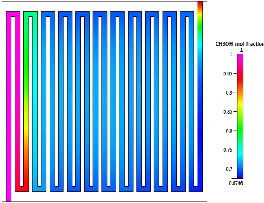
3.3.3 Methanol mole fraction distribution

SSFF1 had a constant distribution of methanol mole fraction of 1 to 0.864 at the anode channel outlet (Figures 19, 20, and 21). This result shows that methanol reacted to generate electric current. The methanol mole fraction distributions of SSFF2 and SSFF3 were not uniform. The mole fraction of methanol dropped significantly before reaching the anode channel outlet. Analysis of pressure and velocity distributions showed that both SSFF2 and SSFF3 had a non-uniform

distribution. Based on this situation, a high possibility exists that SSFF2 and SSFF3 encountered methanol crossover because of the poor methanol transport along the anode channel. Therefore, the SSFF1 design with a channel width of 2.0 mm has the best DMFC performance. The presence of the CO2 in the channel also lead to the limited diffusion rate of

methanol [8] and hence contributes to the non-uniform distribution in the anode channel.

Fig. 19. Methanol mole fraction distribution of SSFF1 (channel width = 2.0 mm)

Fig. 21. Methanol mole fraction distribution of SSFF3 (channel width = 1.0 mm)

3.3.4 Power density comparisons

Comparison of power density shows that SSFF1 had uniform velocity, pressure, and methanol mole fraction distributions. Therefore, SSFF1 is expected to have the highest performance of DMFC. The simulated power densities for all flow fields are shown in Figure 22. In this figure, SSFF1 had the highest value of power density (44.76 mW cm−2), followed by SSFF3 (40.26 mW cm−2) and then SSFF2 (38.19 mW cm−2). These results fit with the expectations based on the CFD indicated earlier, that is, SSFF1 with an optimum channel width of 2.0 mm exhibited a better performance than those with channel widths of 1.0 and 1.5 mm.

Fig. 22. Power density comparisons of SSFF1, SSFF2 and SSFF3 at voltage of 0.261 V

3.3.5 Comparisons of methanol mole fraction distribution at anode catalyst layer

The methanol mole fractions in the anode catalyst layer were compared among SSFF1, SSFF2, and SSFF3 to investigate the cause of high power density production in small channel width of SSFF3 compared to SSFF2. Figures 23, 24, and 25 show the methanol mole fractions in the anode catalyst layers for SSFF1, SSFF2, and SSFF3, respectively. The methanol mole fraction values in SSFF1 were the highest among the three flow fields (Figure 23). This result indicates that a considerable amount of methanol react to generate electricity; thus, the power density was significantly high (Figure 23). The methanol mole fraction of SSFF2 (Figure 24) was lower than that of SSFF3 (Figure 25), which implies that SSFF3 has a higher power density than SSFF2. Compared to Figures 19, 20 and 21, methanol mole fraction distributions at flow field is much higher than in catalyst layer of Figures 23, 24 and 25.

Fig. 24. Methanol mole fraction at anode catalyst layer of SSFF2 Fig. 25. Methanol mole fraction at anode catalyst layer of SSFF3

3.4 Comparisons of power density for all simulated

geometries

Based on the previous analysis, the simulation results showed that SSFF1 with an optimum channel width of 2 mm had the best DMFC performance. The power densities of all simulated geometries were compared. Figure 26 shows the simulation data for the comparisons. SSFF1 obtained the highest power density of 44.76 mW cm−2, followed by SSFF3. The power densities produced in the zigzag flow field and SSFF2 were 38.42 and 38.19 mW cm−2, respectively. PFF exhibited the least power density of 37.81 mW cm−2. These simulation results reveal that PFF is not appropriate for DMFC flow field. The designs developed in this study are suitable for the fundamental understanding of the flow field in DMFC and its visualization of velocity, pressure and methanol mole fraction distributions.

Fig. 26. Power density comparisons of different flow fields at a voltage of 0.261 V

4. CONCLUSIONS

The results show that serpentine flow fields had uniform velocity and methanol mole fraction distributions and a high pressure drop. Such flow fields exhibited the best DMFC performance compared with PFF and zigzag flow field. The serpentine flow field with 2 mm channel width had the best DMFC performance based on its velocity, pressure, and methanol mole fraction distributions, and it is the best flow field simulated in this study. Furthermore, non-uniform distribution of velocity, pressure and methanol mole fraction in PFF and zigzag flow fields confirm the importance of the flow-field in a DMFC design.

ACKNOWLEDGMENT

The authors gratefully acknowledge the financial support of this work by Dana Lonjakan Penerbitan of Universiti Kebangsaan Malaysia (DLP-2014-007) and Fundamental Research Grant Scheme of Ministry of Higher Education Malaysia (FRGS/1/2013/TK07/UKM/02/1).

REFERENCES

[1] H. Yang and T. S. Zhao, "Effect of anode flow field design on the performance of liquid feed direct methanol fuel cells,"

Electrochimica Acta, vol. 50, pp. 3243-3252, 5/30/ 2005. [2] K. Minsu, L. Wonsub, L. Minhye, and M. Il, "3-dimensional CFD

simulation modeling for optimal flow field design of direct methanol fuel cell bipolar plate," in ICCAS-SICE, 2009, 2009, pp. 5463-5468.

[3] V. A. Danilov, J. Lim, I. Moon, and H. Chang, "Three-dimensional, two-phase, CFD model for the design of a direct methanol fuel cell," Journal of Power Sources, vol. 162, pp. 992-1002, 11/22/ 2006.

[4] C. W. Wong, T. S. Zhao, Q. Ye, and J. G. Liu, "Experimental investigations of the anode flow field of a micro direct methanol fuel cell," Journal of Power Sources, vol. 155, pp. 291-296, 4/21/ 2006.

[6] A. S. Aric , . Cret , . Baglio, E. Modica, and V. Antonucci, "Influence of flow field design on the performance of a direct methanol fuel cell," Journal of Power Sources, vol. 91, pp. 202-209, 12// 2000.

[7] T. J. Chung, Computational Fluid Dynamics. United Kingdom: Cambridge University Press, 2010.

[8] Y.-C. Park, P. Chippar, S.-K. Kim, S. Lim, D.-H. Jung, H. Ju, et al., "Effects of serpentine flow-field designs with different channel and rib widths on the performance of a direct methanol fuel cell,"

Journal of Power Sources, vol. 205, pp. 32-47, 5/1/ 2012. [9] ESI-CFD, "CFD-ACE+ V2014.0 User Manual," ed. Huntsville,

AL: ESI-CFD, Inc., 2014.

[10] B. Yu, Q. Yang, A. Kianimanesh, T. Freiheit, S. S. Park, H. Zhao, et al., "A CFD model with semi-empirical electrochemical relationships to study the influence of geometric and operating parameters on DMFC performance," International Journal of Hydrogen Energy, vol. 38, pp. 9873-9885, 8/6/ 2013.

[11] W. W. Yang, Y. L. He, and Y. S. Li, "Modeling of dynamic operating behaviors in a liquid-feed direct methanol fuel cell,"

International Journal of Hydrogen Energy, vol. 37, pp. 18412-18424, 12// 2012.

[12] M.-s. Hyun, S.-K. Kim, D. Jung, B. Lee, D. Peck, T. Kim, et al., "Prediction of anode performances of direct methanol fuel cells with different flow-field design using computational simulation,"