Watermarking Algorithm Using Sobel Edge
Detection
P. Ramesh Kumar
Department of Computer Science and Engineering, V.R.Siddhartha Engineering College, Vijayawada, INDIA Email: [email protected]
K.L.Sailaja
Department of Computer Science and Engineering, V.R.Siddhartha Engineering College, Vijayawada, INDIA Email: [email protected]
---ABSTRACT--- Digital Watermarking is a process of embedding information into a digital signal. The efficiency of the watermarking process depends on the protection of visually significant information. For that we embed the watermark transparently at the edges of digital image where deformation is less identifiable. To identify the edges we used Sobel edge detection algorithm since it is inexpensive in terms of computations and on the other hand, the gradient approximation which it produces is relatively crude, in particular for high frequency variations in the image.
Keywords – Watermarking, Wavelet Transform, Edge Detection.
--- Date of Submission 14 July 2010 Revised: 02 November 2010 Date of Acceptance: 29 December 2010 ---
1. INTRODUCTION
I
n today's Internet environment, Digital images facilitate efficient distribution, reproduction, and manipulation over networked information systems. However, these efficiencies also increase the problems associated with copyright enforcement [1]. The recent growth of networked multimedia systems has caused problems relative to the protection of intellectual property rights. This is particularly true for image and video data. Adequate protection of digital copies of multimedia content is a prerequisite to the distribution over network. The growth of networked multimedia systems has magnified the need for image copyright protection. One approach used to address this problem is to add an invisible structure to an image that can be used to seal or mark it.In visible watermarking, the information is visible in the picture or video. Typically, the information is text or a logo which identifies the owner of the media where as in invisible watermarking, information is added as digital data to audio, picture or video, but it cannot be perceived as such (although it is possible to detect the hidden information). An important application of invisible watermarking is to copyright protection systems, which are intended to prevent or deter unauthorized copying of digital media.
Fig 1: Visible and Invisible watermarked Images
The digital image watermarking techniques in the literature are typically grouped in two classes: Spatial domain techniques [2] [3] [4]: which embed the watermark by modifying the pixel values of the original image and the transform domain techniques which embed the watermark in the domain of an invertible transform. The discrete cosine transform (DCT) and the discrete wavelet transform (DWT) [5]-[13] are commonly used for watermarking purposes.
The transform domain algorithms modify a subset of the transform coefficients with the watermarking data and generally achieve better robustness than spatial domain methods.
A. Discrete Cosine Transform (DCT)
The following equation computes the DCT coefficients of an m x n image
(
)
( )
0 11 0 1
0 1 0
,
2
1
2
cos
2
1
2
cos
≤≤≤≤−−−
= −
=
+
∏
+
∏
=
∑
∑
PMN q N
n mn M
m q p pq
N
n
M
P
m
A
B
α
α
(1)0
1 1
1
2
=
− ≤ ≤
=
P
M P M
M P
α
(2)0
1 1 1
2
=
− ≤ ≤
=
q
N q N
N q
α
(3)Where M and N are the row and the column size of A respectively.
B. Discrete Wavelet Transform (DWT)
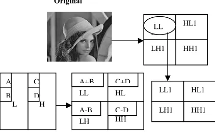
Initially, the input image is decomposed into four levels by a DWT, resulting in an approximation subband with low frequency components and 12 detail subbands with high frequency components.
Fig 2: 1-Level Decomposition of Input Image
Fig 3: 2-Level Decomposition of Input Image
2. ALGORITHMSFOREDGEDETECTION
A. Introduction to Fundamentals of Edge Detection
Since edge detection is in the forefront of image
processing for object detection, it is crucial to have a good understanding of edge detection algorithms. Edges in images are areas with strong intensity contrasts. Edge detection refers to the process of identifying and locating sharp discontinuities in an image. The discontinuities are abrupt changes in pixel intensity which characterize boundaries of objects in a scene. Classical methods of edge detection involve convolving the image with an operator. There is an extremely large number of edge detection operators available, each designed to be sensitive to certain types of edges. Variables involved in the selection of an edge detection operator include:• Edge orientation: The geometry of the operator determines a characteristic direction in which it is most sensitive to edges. Operators can be optimized to look for horizontal, vertical, or diagonal edges.
• Noise environment: Operators used on noisy images are typically larger in scope, so they can average enough data to discount localized noisy pixels. This results in less accurate localization of the detected edges.
• Edge structure: Not all edges involve a step change in intensity. Effects such as refraction or poor focus can result in objects with boundaries defined by a gradual change in intensity. The operator needs to be chosen to be responsive to such a gradual change in those cases.
B. Various Methods to perform Edge Detection
A variety of Edge Detectors are available for detecting the edges in digital images. However, each detector has its own advantages and disadvantages. The basic idea behind edge detection is to find places in an image where the intensity changes rapidly.
Edge detecting an image significantly reduces the amount of data and filters out useless information, while preserving the important structural properties in an image. There are many ways to perform edge detection. The edge Detection methods may be grouped into two categories, Gradient and Laplacian each designed to be sensitive to certain types of edges.
• Gradient: The gradient method detects the edges by looking for the maximum and minimum in the first derivative of the image. Roberts, Prewitt and Sobel come under Gradient method.
• Laplacian: The Laplacian method searches for zero crossings in the second derivative of the image to find edges. An edge has the one-dimensional shape of a ramp and calculating the derivative of the image can highlight its location. Marrs-Hildreth edge detection comes under Laplacian.
LL1 HL1
HH1 LH1
LL
LL1 HL1
HH1 LH1 L H
A B
C
D LL HL
HH LH
A+B C+D
A-B C-D
Original
3. SOBELEDGEDETECTIONTECHNIQUE
A. Sobel Operator
The Sobel operator is used in image processing, particularly within edge detection algorithms. Technically, it is a discrete differentiation operator computing an approximation of the gradient of the image intensity function. At each point in the image, the result of the Sobel operator is either the corresponding gradient vector or the norm of this vector. The Sobel operator is based on convolving the image with a small, separable, and integer valued filter in horizontal and vertical direction.
B. Simplified Description
The operator calculates the gradient of the image intensity at each point, giving the direction of the largest possible increase from light to dark and the rate of change in that direction. The result therefore shows how smoothly the image changes at that point and therefore how likely it is that part of the image represents an edge, as well as how that edge is likely to be oriented.
Mathematically, the gradient of a two-variable function is at each image point a 2D vector with the components given by the derivatives in the horizontal and vertical directions. At each image point, the gradient vector points in the direction of largest possible intensity increase, and the length of the gradient vector corresponds to the rate of change in that direction. This implies that the result of the Sobel operator at an image point which is in a region of constant image intensity is a zero vector and at a point on an edge is a vector which points across the edge, from darker to brighter values.
C. Formulation
The operator consists of a pair of 3×3 convolution kernels as shown in Figure 3.3.1. One kernel is simply the other rotated by 90°.
These kernels are designed to respond maximally to edges running vertically and horizontally relative to the pixel grid, one kernel for each of the two perpendicular orientations. The kernels can be applied separately to the input image, to produce separate measurements of the gradient component in each orientation (Gx and Gy). Mathematically, the operator uses two 3×3 kernels which are convolved with the original image to calculate approximations of the derivatives - one for horizontal changes, and one for vertical. If we define A as the source image, and Gx and Gy are two images which at each point
contain the horizontal and vertical derivative approximations, the computations are as follows:
− − − + + + = 1 2 1 0 0 0 1 2 1 8 1 y
G * A and
− + − + − + = 1 0 1 2 0 2 1 0 1 8 1 x
G * A
Where * here denotes the 2-dimensional convolution operation.
The x-coordinate is here defined as increasing in the "right"-direction, and the y-coordinate is defined as increasing in the "down"-direction. At each point in the image, the resulting gradient approximations can be combined to give the gradient magnitude, using:
G
=
(
G
x2+
G
y2)
(4)
Using this information, we can also calculate the gradient's direction:
=
x yG
G
arctan
θ
(5)Where Θ is 0 for a vertical edge which is darker on the left side.
Since the intensity function of a digital image is only known at discrete points, derivatives of this function cannot be defined unless we assume that there is an underlying continuous intensity function which has been sampled at the image points. With some additional assumptions, the derivative of the continuous intensity function can be computed as a function on the sampled intensity function. It turns out that the derivatives at any particular point are functions of the intensity values at virtually all image points. However, approximations of these derivative functions can be defined at lesser or larger degrees of accuracy.
The Sobel operator uses intensity values only in a 3×3 region around each image point to approximate the corresponding image gradient, and it uses only integer values for the coefficients which weight the image intensities to produce the gradient approximation.
D. Technical details
The Sobel operator can be implemented by simple means in both hardware and software: only eight image points around a point are needed to compute the corresponding result and only integer arithmetic is needed to compute the gradient vector approximation. Furthermore, the two discrete filters described above are both separable:
[
1 0 1]
1 2 1 1 0 1 2 0 2 1 0 1 − + = − + − + − +
[
1 2 1]
1 0 1 1 2 1 0 0 0 1 2 1 − + = − − − + + +
and the two derivatives Gx and Gy can therefore be
computed as -1 0 +1
-2 0 +2 -1 0 +1
[
]
(
A)
Gx * 1 0 1* 1
2 1
− +
= Gx *
(
[
1 2 1]
*A)
1 0
1
− + =
This separable computation may be advantageous since it implies fewer arithmetic computations for each image point. The result of the Sobel operator is a 2-dimensional map of the gradient at each point. It can be processed and viewed as though it is itself an image, with the areas of high gradient (the likely edges) visible as white lines.
Fig 4: Detection of edges using Sobel method
E. Sobel Explanation
The mask is slid over an area of the input image, changes that pixel's value and then shifts one pixel to the right and continues to the right until it reaches the end of a row. It then starts at the beginning of the next row.
The example below shows the mask being slid over the top left portion of the input image represented by the green outline. The formula shows how a particular pixel in the output image would be calculated. The center of the mask is placed over the pixel you are manipulating in the image. And the I & J values are used to move the file pointer so you can multiply, for example, pixel (a22) by the corresponding mask value (m22).
The pixels in the first and last rows, as well as the first and last columns cannot be manipulated by a 3x3 mask. This is because when placing the center of the mask over a pixel in the first row (for example), the mask will be outside the image boundaries.
The GX mask highlights the edges in the horizontal direction while the GY mask highlights the edges in the vertical direction. After taking the magnitude of both, the resulting output detects edges in both directions.
Input image Mask
Output Image 4. EXISTINGSYSTEM
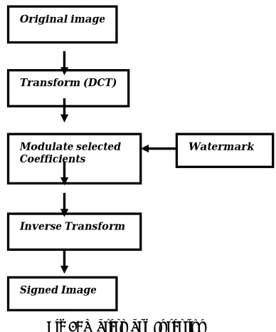
The Existing system of digital watermarking uses DCT with which we first perform DCT on the original image to get the modulated coefficients on which the watermark is inserted and apply IDCT in ordered to generate the signed version of the original image that contains the watermark.
Fig 5: Watermark Insertion
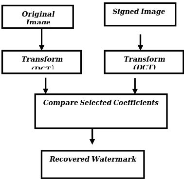
In the recovery of the watermark we perform DCT on the original image as well as on the signed image and then compare the selected Coefficients. If the coefficients contain same value then watermark is recovered.
a11 a12 a13 … A1n
a21 a22 a23 … A2n
a31 a32 a33 … A11
m11 m12 m13
m21 m22 m23
m31 m32 m33
b11 b12 b13 … b1n
b21 b22 b23 … b2n
b31 b32 b33 … a11
Original image
Transform (DCT)
Modulate selected
Coefficients Watermark
Inverse Transform
Fig 6: Watermark Detection
5. THEPROPOSEDALGORITHM
A. The Watermark Insertion Process
In the watermark insertion process, we apply a 2-level DWT decomposition on the original input image I. The important wavelet coefficients at the edge of the input image are detected by Sobel edge detector.
Fig 7: Watermark Insertion Process
The original input image is subjected to 2 level DWT to obtain the Co-efficients and apply Sobel Edge Detection method to obtain the Edge Co-efficients. Insert the Watermark to the selected Edge coefficients. Adding the watermark to these edge coefficients makes the insertion
invisible to the human visual system as distortions are less noticeable at edges.
When inserting the watermark a series of coefficients are extracted from the image’s DWT domain. Let the image be denoted by I and the series of coefficients be C = c1, c2,….cn where n is the length of watermark. Before watermarking the image I it has to be subjected to a 2 Level DWT transformation. Then significant coefficients are obtained. These coefficients are subjected to pass through Sobel Edge detection then edge coefficients are obtained. The watermark can be inserted by altering the coefficients by the following formula:
C
N i =C
O i+G W
i (6)Where • CNi - i
th
wavelet coefficient of watermarked Image.
• COi - ith Edge wavelet coefficient of Original
Image by Sobel methods
• G – Gradient value range from 0 to 1
• Wi –
ith Watermark coefficient to be inserted.
B. The Watermark Extraction Process
Watermark detection is performed by extracting wavelet coefficient from the Watermarked image using DWT and subtracting original edge wavelet co-efficient to get the exact watermark. Fig. 8 shows
Fig 8: Watermark Extraction Process
Original Image
Transform
(DCT)
Signed Image
Transform (DCT)
Compare Selected Coefficients
Recovered Watermark
Watermark
1st Level
DWT
2nd Level
DWT
Co-efficients of Input image
Sobel Edge Detection
method
Watermark Insertion
Process
Watermarke d Image Input
Image
Edge Co-efficients of
Input image
Watermark
1st Level
DWT
2nd Level
DWT
Co-efficient of watermarked
image Sobel Edge
Detection method
Watermark Detection Process
Watermarke d Image Input
Image
Edge Co-efficient
of
1st Level
DWT
2nd Level
From equation (6) we can take the logarithm of Edge wavelet coefficient of original image to get:
C
O i =C
O iexp ( G W
i ) (7)From equation (7) an inverse insertion function can easily be found to be:
W
i*= ( CN i*- C
O i) / ( G W
i ) (8)Where
C
N i*are the extracted wavelet coefficients from the watermarked images DWT domain. From equation (8) we see that the original Edge wavelet coefficients CO i are needed therefore we need the original image and W i *extracted watermark [6].
6. EXPERIMENTALRESULTS
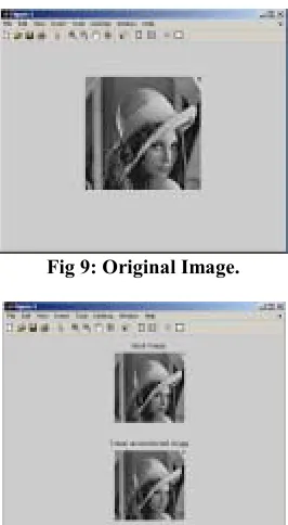
The proposed method is evaluated on the image: “Lena”, which is an image with large smooth regions. The performance measures are the invisibility of the inserted watermark and the robustness of the method against various types of attacks.
Fig. 9 shows the original image of “Lena” and its watermarked copy, whereas Fig. 10 shows their difference. The watermarked copy is undistinguishable from the original image. In the difference, which is suitably scaled for display, it is evident that watermark data are added to the edges where they are perceptually invisible.
Fig 9: Original Image.
Fig 10: Image after applying 1 Level DWT
Fig 11: Image after applying 2 Level DWT
Fig 12: Detecting the Edges by applying Sobel Edge Detection Algorithm
Fig 14: Watermark Extracted.
7.CONCLUSION
In the article, a method for image watermarking has been presented. The method inserts the watermarking data on the Edge coefficients of the input image. Edge coefficients are formed after detecting the edges using a Sobel edge detection method. Since the watermark is inserted at the Edges of the input image, the distortions in the watermarked image are less noticeable.
The watermark extraction method needs the original input image to extract the watermark. The proposed method shows good performance as far as invisibility is concerned. References
[1] John N. Ellinas “A Robust Wavelet-Based Watermarking Algorithm Using Edge Detection” Proc.world Academy Science, Engineering and Technology, 2007, Vol.25, pp 439-443.
[2] R. Schyndel, A. Tirkel, and C. Osborne, “A digital watermark,” in IEEE Proc. Int. Conf. Image Processing, 1994, vol. 2, pp. 86–90.
[3] W. Bender, D. Gruhl, N. Morimoto, and A. Lu, “Techniques for data hiding,” IBM Systems Journal, vol. 35, no. 3-4, pp. 313-336, 1996.
[4] R. B. Wolfgang and E. J. Delp, “A watermark for digital images,” in IEEE Proc. Int. Conf. Image Processing, 1996, vol. 3, pp. 219–222.
[5] M. D. Swanson, B. Zhu, and A. H. Tewfik, “Transparent robust image watermarking,” in IEEE Proc. Int. Conf. Image Processing, 1996, vol. 3, pp. 211–214.
[6] J. Cox, J. Kilian, T. Leighton, and T. Shamoon, “Secure spread watermarking for multimedia,” IEEE Trans. Image Processing, vol. 6, no. 12, pp. 1673– 1687, Dec. 1997.
[7] M. Barni, F. Bartolini,a and A. Piva, “Improved wavelet-based watermarking through pixel-wise masking”, IEEE Trans. Image Processing, vol. 10, no. 5, pp. 783–791, 2001.
[8] X. Xia, C. G. Boncelet, and G. R. Arce, “A multiresolution watermark for digital images,” in IEEE Proc. Int. Conf. Image Processing, USA, 1997, pp. 548-551.
[9] J. R. Kim, and Y. S. Moon, “A robust wavelet-based digital watermarking using level-adaptive thresholding,” in IEEE Proc. Int. Conf. Image Processing, Japan, 1999, pp. 226-230.
[10] T. Hsu, and J. L. Wu, “Hidden digital watermarks in images,” IEEE Trans. Image Processing, vol. 8, no. 1, pp. 58–68, Jan. 1999.
[11] R. Dugad, K. Ratakonda, and N. Ahuja, “A new wavelet-based scheme for watermarking images,” in IEEE Proc. Int. Conf. Image Processing,USA, 1998, pp. 419-423.
[12] R. B. Wolfgang, C. I. Podilchuk, and E. J. Delp, “Perceptual watermarks for digital images and video,” in SPIE Proc. Int. Conf. Security and watermarking of multimedia contents, USA, 1999, pp. 40-51.
[13] J. N. Ellinas, D. E. Manolakis, “A robust watermarking scheme based on edge detection and contrast sensitivity function,” in VISAPP Proc. Int.Conf. Computer Vision Theory and Applications, Barcelona, 2007.
Authors Biography
Ramesh Kumar .P received B.Tech (CSE), M.Tech (CSE). He is currently serving as Sr.Lecturer in the Department of Computer Science and Engineering, V.R.Siddhartha Engineering College. His research interest lies in the area of Ear Biometrics and Cryptography, Parallel Computing and Key Management. Member of CSI, IETE and ISTE.
K.L.Sailaja received her B.Tech (CSE), M.Tech (CSE). She is currently working as