Intermolecular interactions using molecular quantum electrodynamics

INTERMOLECULAR INTERACTIONS USING MOLECULAR QUANTUM ELECTRODYNAMICS

by

Agha Akbar SALAM

A thesis submitted in partial fulfilment of the requirements of the University of London for the

degree of Doctor of Philosophy, October, 1993.

P roQ uest Num ber: 10017782

All rights reserved

IN F O R M A T IO N T O ALL U S E R S

T h e quality of this reproduction is d ep en d en t upon the quality of the copy subm itted.

In the unlikely event that the author did not send a com plete m anuscript

and there are missing pages, these will be noted. Also, if m aterial had to be rem oved, a note will indicate the deletion.

uest.

P roQ uest 10017782

Published by P roQ uest LL C (2016). Copyright of the Dissertation is held by the Author.

All rights reserved.

This work is protected against unauthorized copying under Title 17, United States C ode.

Microform Edition © P roQ uest LLC.

ProQ uest LLC

789 East E isenhow er P arkw ay

"Mathematics is the tool specially suited for dealing with abstract concepts of any kind and there is no limit to its power in this field. For this reason a book on the new physics, if not purely descriptive of experimental work, must be essentially mathematical. All the same the mathematics is only a tool and one should learn to hold the physical

ideas in one’s mind without reference to the mathematical form."

P.A.M. Dirac,

ABSTRACT

The physical theory describing the interaction of electromagnetic radiation with atoms and molecules, molecular quantum electrodynamics, is applied to problems in intermolecular interactions and optical activity.

After an outline of the basic Coulomb gauge theory in Chapter 1, the quantum electrodynamical Maxwell field operators in the vicinity of a molecule are derived in Chapter 2 in both the multipolar and minimal-coupling frameworks in the Heisenberg picture. The electromagnetic field operators are expanded in powers of the transition moments, correct up to second order in the sources with the interaction Hamiltonian including electric dipole and quadrupole, magnetic dipole and diamagnetic coupling terms.

The Maxwell field operators in the multipolar form are then used in Chapter 3 to calculate the Thompson energy density and the Poynting vector associated with the electromagnetic field. The equivalence of the expectation value of both these operators obtained using the minimal-coupling Maxwell fields in the electric dipole approximation is demonstrated.

The near- and far-zone behaviour is also examined.

ACKNOWLEDGEMENTS

I express my sincerest thanks to Dr T. Thirunamachandran for his stimulating teaching, throughout the duration of my studies at the Department of Chemistry, in addition to his patience and generosity while supervising this research.

I also thank the many members of staff, most notably Dr S.H. Walmsley, past and present occupants of the G25 Theoretical Laboratory, and finally, many friends, too numerous to mention, all of whom have made the six years that I have spent at UCL most enjoyable.

CONTENTS

Page

ABSTRACT 3

ACKNOWLEDGEMENTS 5

CONTENTS 6

CHAPTER 1

COULOMB G\UGE QUANTUM ELECTRODYNAMICS

1.1 Introduction 8

1.2 Basic Theory 10

1.3 Applications 24

CHAPTER 2

ELECTROMAGNETIC FIELDS IN THE NEIGHBOURHOOD OF A MOLECULE

2.1 Introduction 26

2.2 Maxwell Fields From Multipolar Hamiltonian 28 2.3 Maxwell Fields From Minimal-Coupling Hamiltonian 53

Appendix 77

CHAPTER 3

ENERGY DENSITIES AND POYNTING \TCTOR

3.1 Introduction 81

3.2 Energy Density Using Multipolar Maxwell Fields 88 3.3 Energy Density Using Minimal-Coupling Maxwell Fields 112 3.4 Energy Flux Using Multipolar Maxwell Fields 118 3.5 Energy Flux Using Minimal-Coupling Maxwell Fields 131

CHAPTER 4

INTEPu^CTION OF TWO POL\RIS.\BLE MOLECULES

4.1 Introduction 137

4.2 The Interaction Between Two Electric Dipole 141 Polarisable Molecules

4.3 The Interaction Between A Chiral Molecule And An 151 Electric Dipole Polarisable Molecule

4.4 The Interaction Between An Electric Dipole Polarisable Molecule 154 And An Electric Dipole-Quadrupole Polarisable Molecule

4.5 The Interaction Between Two Chiral Molecules 157 4.6 The Interaction Between An Electric Dipole Polarisable 163

Molecule And A Magnetic Dipole Polarisable Molecule

4.7 The Interaction Between An Electric Dipole Polarisable 168 Molecule And An Electric Quadrupole Polarisable Molecule

4.8 The Interaction Between Two Electric Dipole-Quadrupole 173 Polarisable Molecules

4.9 The Interaction Between An Electric Dipole Polarisable Molecule 176 And A Magnetic Dipole-Electric Quadrupole Polarisable Molecule

4.10 The Interaction Between A Chiral Molecule And An Electric 179 Dipole-Quadrupole Polarisable Molecule

4.11 Contribution From The Diamagnetic Coupling Term 182 4.12 Near-Zone Limit To The Dispersion Interaction 184

Appendix 191

CHAPTER 5

MOLECULE INDUCED CIRCUL<U)LY POLARISED LUMINESCENCE

5.1 Introduction 201

5.2 Evaluation Of Matrix Element In The Schrodinger Picture 203 5.3 Evaluation Of Matrix Element In The Heisenberg Picture 209 5.4 Evaluation Of Differential Emission Rate 212

CHAPTER 1

COULOMB GAUGE QUANTUM ELECTRODYNAMICS

1.1 INTRODUCTION

Quantum electrodynamics (OED) is the physical theory that describes the interaction of matter with electromagnetic fields and the interaction between atoms and molecules.

The origins of OED lie in the fundamental paper by Dirac [1] in which the radiation field is treated quantum mechanically. This process, known as second quantisation, gives rise to the quantised particle of radiation called the photon. The need for a quantum field theory arose from the singular failure of semi-classical theory to account for spontaneous emission. The quantum theory of radiation not only enabled the Einstein A- and B-coefficients to be derived in a straightforward manner, but further accounted for previously inexplicable phenomena such as the anomalous magnetic moment of the electron, and the Lamb shift, where the agreement between theory and experiment has been excellent. Of the theories currently available, QED, either formulated using traditional field theory or the alternative space-time approach due to Feynman [2,3], provides the most accurate description of photon-electron interactions known so far.

field alone and a small term representing the coupling energy of the particles and the field.

In chemical physics, where the problem is the coupling of radiation with particles of low energy, a non-covariant formulation of QED is sufficient. A theory of the emission and absorption of radiation and of the reaction of the radiation field on the system has been built up on the basis of a dynamics which is not relativistic [1,4]. This is on account of the time being treated throughout as a c-number instead of symmetrically with the space coordinates. Molecular QED is the non-relativistic limit of QED, and is applied to systems involving bound electrons of low binding energies moving with velocities insignificant to that of light, making it ideally suited to the study of problems of chemical interest. To facilitate the use of molecular QED in the non-covariant version, the Coulomb gauge condition is employed throughout, allowing separation of the dynamic and static aspects of the sources of the field.

QED may be formulated in either the Schrodinger or Heisenberg representations. Almost all the applications of molecular QED to date have been investigated in the more familiar Schrodinger picture. In this thesis, the alternative Heisenberg viewpoint is employed in dealing with radiation-molecule interactions.

those by Power [5], Craig and Thirunamachandran [6,7], Healy [8], Andrews et al. [9], Woolley [10], Cohen-Tannoudji et al, [11] and the compilation by Schwinger [12].

After a brief outline of the basic QED theory in the subsequent Section, a detailed exposition in the Heisenberg framework is given in Chapter 2.

1.2 BASIC THEORY

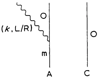
Consider a collection of slowly moving charged particles ot of charge e^, mass m^ with position q^ and velocity q^, interacting with the radiation field of vector potential a(r) subject to the Coulomb gauge condition

'7, a( r ) = 0. (1.2.1)

Classically, the total system is described by the Lagrangian [13]

-j. £ ^

L = 1/22 "V + ja(r)“-c“(^>^a(r) )“jd“r + Jj (r).a(r)dr (1.2.2)

in which V is the electrostatic potential energy and j'*’(f) is the transverse part of the total current density

j(r) = • (1.2.3)

a

Lagrangian is a function of the coordinates and velocities of the particle and a functional of the corresponding field "coordinates and velocities". In the absence of interaction, only the particles Lagrangian and the free field Lagrangian remain, with the dynamics of one system not affecting that of the other. The two systems move independently and have equations of motion that are not coupled to one another. When the particles and field interact, the coupling appears as an interaction term in the Lagrangian. The specific choice of Lagrangian is such that it leads to the correct equations of motion. By invoking Hamilton's principle through the calculus of variations, the solutions of which are Lagrange's equations of motion [14], it can be shown, that in this case the equations of motion lead to the Lorentz force for particles (1.2.4) and to Maxwell’s equations, with sources, for the radiation field (1.2.5).

v i a " - (1.2.4)

e( r ) P(r)

u.b(r) = 0

(1.2.5)

at

e'*"(r) = — à(r) (1.2.6)

^(r) = V*â(r). (1.2.7)

The transverse component of e(r) is a consequence of the gauge condition (1.2.1). The charge density is

p(r ) = ^e^0(i;-q^). (1.2.8)

a

The equations of motion may be written in an alternative manner by starting from an arbitrary gauge with the introduction of the electromagnetic potentials [15,16], which also aid the subsequent quantisation of the electromagnetic field. From the second equation of

(1.2.5) it is seen that the definition of the vector potential (1.2.7) still holds. Substituting this into the third equation of (1.2.5) and noting that a vector whose curl is zero can be defined as the gradient of a scalar function,

e(r) + a(r) = -V#(r) , (1.2.9)

where 0(r) is the scalar potential. The electromagnetic potentials as defined by (1.2.6) and (1.2.7) are not unique, being determined up to an additive gauge function X, expressed in the gauge transformation

a(r) ^ a(r) + ?X i $(rl =» <t>(r) - i

the treatment of atoms and molecules requires an explicit Coulomb potential term in the Hamiltonian, the choice of X given by

leads to the Coulomb gauge defined earlier. The equations of motion in terms of the potentials are obtained from the remaining Maxwell equations after decomposition of the electric field into longitudinal and transverse parts [17], and are

a(r) = ---- ^j'*’(r) (1.2.12)

V “0(?) = -p(?)/Eg. (1.2.13)

The choice of Coulomb gauge thus separates the Coulombic fields from the transverse fields;

e‘*'(r) = -à(r) ; é” (r) = -'^0(r). (1.2.14)

The electrostatic field due to the charged particles is given by e"(r) and described by the scalar potential while the radiation field e^(r) is described by the transverse vector potential.

The Lagrangian function expressed in terms of the electromagnetic potentials which leads to the equations of motion (1.2.12) and (1.2.13)

is

and is known as the Coulomb gauge Lagrangian. The scalar potential 0(r) may be eliminated from (1.2.15) in favour of the electrostatic potential energy V by employing the relationship of the latter to the longitudinal electric field. This results in the Lagrangian (1.2.2), which is known as the minimal-coupling Lagrangian.

It is possible in an alternative formulation to describe the equations of motion using the Hamiltonian function [14], defined in terms of the Lagrangian by

H = ^ Pg.q^ + Jrt(r).a(r)d^r - L. (1.2.16)

Of

The dynamical variables are then the generalised coordinates and the canonically conjugate momenta, which for particles and field are respectively given by

P« = ; rt(r) = ^ , (1.2.17)

(1.2.18)

= ih5^:(r-r'), (1.2.19)

where 5"^-(f^r') is the transverse delta-dyadic [5]. Thus the minimal-coupling Hamiltonian [6]

'«IN = I "MOl'CI + «RAD + I ^I N T E R ’ (1.2.2 0)

with

+ V(C) (1.2.2 1)

, ^ 1

RAD 2 (1.2.2 2)

-

2

a a

(1.2.23)

and

ViNTER -

1

(1.2.24)

vector potential while the second order term, quadratic in the electric charge depends on the square of the vector potential. The potential term appears explicitly in the Hamiltonian and is separated into intra- and inter-molecular contributions.

The application of molecular OED to problems in chemical physics is facilitated by the use of the multipolar Hamiltonian [20]. In this framework radiation-molecule interactions are described solely by the coupling of molecular multipoles to the electric displacement and magnetic fields. The multipolar Lagrangian, used to determine the multipolar Hamiltonian, is obtained from the minimal-coupling Lagrangian by the addition of a total time derivative of a function of the coordinates [21]. The transformation uses the property that the equations of motion derived from a Lagrangian are unaltered by just such an addition. Lagrangians so related are said to be equivalent, but give rise to Hamiltonians differing in form. Thus

^«ULT = L„in - (1.2.25)

where p(r) is the electric polarisation field and is a function of the particle coordinates. The multipolar Lagrangian is then written as

^ U L T = 2 - V C ) } + C ' a

-Jp'*’( r ).à(r)d^r + J^9xW(r)j.a(r)d^r - 2 ^ (1.2.26) C<C'

where p(r), and the magnetisation field M(r), are defined by

p(r) = y p(C;r); M(r) = ^ M(C;r) (1.2.27)

with

p(Ç;r) = J e^(q^(C)-S-)| 6(r-t--X(q^(Ç)-R.))dX , (1.2.28)

oc

and

M( Ç;?) = 2 >^^(r-3ç-X(q„(Ç)-Sç))dX . (1.2.29)

These fields allow the total charge density associated with each ensemble to be partitioned into true and polarisation charge densities, and the total current density into true, polarisation and magnetisation current densities [22,23]. This division of the sources necessitates the introduction of a reference vector which may conveniently be taken as the centre of mass, an inversion centre or a local chromophore centre.

The multipolar Hamiltonian [24], evaluated in the usual manner gives

"MULT = 1 + «RAD + 1 + "sELF '1'^ '^0>

c

c

with unchanged from (1.2.21)

H - 1

“r a d 2 + G„c"b"(?))>d"r (1.2.31)

0

(r) ^ , 22 -O " ' '■ J

and the interaction terms now given by

j p ( r ). d'*’( r )d“r - J m ( f). b( r )d^r

+ ^|o^--(r,r')b^(r )b .(r')d^rd^r'. (1.2.33)

It should be noted that in the multipolar framework it is the transverse electric displacement vector field d'*’(r) that appears explicitly, rather than the transverse electric field e^(r) as found in The displacement vector is defined as

d(r) = Egéfr) + p(r). (1.2.34)

The quantum mechanical mode expansions for the electromagnetic fields d (r ) and b(r) are

k, k

(1.2.35)

k,X

(1.2.36)

The creation and annihilation operators are subject to the commutation relation

= X' ' (1.2.38)

The first term of (1.2.33) denotes the interaction of the electric multipoles with the transverse electric displacement field. The second term represents the interaction of the magnetic multipoles with the magnetic field. The modified magnetisation field is defined as

m(r) = 2 m(C;r) (1.2.39)

w i th

f \

m(C;r) = 2 “ P«(C)*n^(r;r)j. (1.2.40)

In (1.2.40) the vector field n(C;r) for a molecule

C

n(r) = ) n(C;r) (1.2.41)

n^(C,r) = > e^(a (C)-R.) X0{ r-R-->-( q^( O ) )dX . (1.2.42)

OC t _ O C J C ^ 0 s

oc

defined as

Oy^.(r,r') = 2 ; r» r') (1.2.43)

C,C'

<)ylC,C';r,?'l = >• (1.2.44)

(X

The term is independent of the electromagnetic field and does not play an important role in radiative processes and for this reason is usually neglected. It must however be incorporated into self energy calculations as in the treatment of the Lamb shift.

The particular choice of the total time derivative in (1.2.25) leads to the elimination of the intermolecular Coulomb interactions in the resulting multipolar Hamiltonian describing neutral systems, a characteristic feature of this approach. Molecules couple entirely to the electric displacement and magnetic fields and all intermolecular interactions are mediated by the exchange of transverse photons. Thus retardation is a natural occurrence in the multipolar formalism with signals propagating at the speed of light.

It has been demonstrated how the multipolar Hamiltonian may be obtained from the minimal coupling Lagrangian by the addition of a total time derivative followed by the construction of the Hamiltonian

from L„.,,^. An alternative method of obtaining H^,,, ^ is to start with

M U L T M U L T

the minimal coupling Hamiltonian H^^^, found from L, and then to apply

MIN MIN

a canonical transformation [20,25-29] on H^,^, to find

MIN MULL

quantum analogues of contact transformations in classical theory [14,18]. The transformation which results in when applied to

M U L l M I N

is

H « u l t = - (1-2-4 5)

with the particular choice of generator

S = l/hjp^(r).a(r)d"r . (1,2.46)

It is clear that q and à(r) remain unaltered by the transformation with only the corresponding momenta changing. The resulting multipolar Hamiltonian is that given by (1.2.30). It should be noted that although the partitioning of the minimal- and multipolar-coupling Hamiltonians is different in both cases, identical matrix elements are obtained for processes where conservation of energy hold. This is a consequence of the two forms of Hamiltonian being equivalent, thus giving equal matrix elements "on the energy shell".

The interaction terra of the Hamiltonian (1.2.33) is conveniently expanded in terms of multipole moments to simplify its subsequent use in the applications to be considered. The leading contributions to the multipolar series of the polarisation and magnetisation fields, and the ones emnloyed in this thesis are

p.(C;D = (u.(Ç) - Q;;(C)V- + . ..)5(r-a_) (1.2.47)

e r 'i

«D1A<^> = z 8 y ' 9 « ' 0 - R g ) x b ( R ^ ) j . (1.2.49) (Y

In (1.2.47) and in the rest of this thesis, the Einstein summation convention is used. The electric dipole, electric quadrupole and magnetic dipole moments of molecule C are respectively given by

= 2 (1.2.50)

8 ^ / 0 = i I (1.2.51)

\

Using the definitions above in (1.2.33) and performing the volume integral, the multipolar interaction Hamiltonian becomes

= - £'’m(C).3-"(Sç) - e'’Q^^(C)V <j;J;(Sç) - mlC).b(g^l

+ y 5 ^ |(q^(C)-fiç)xb(Rç)| (1.2.53) - -’"a

a

including all terms of a similar origîfi. Assuming that the coupling between radiation and matter is small enough to be considered as a perturbation on the system, both the minimal-coupling and the multipolar Hamiltonians may be suitably divided as

with

H,NT = 2 + V,NTER' '1-2-56)

c

remembering that is absent in the multipolar case. The base states are then given by the eigenstates of which are the products of the eigenstates of the unperturbed molecular and radiation field Hamiltonians, whose solutions are taken to be known. For processes dependent upon time, the perturbation causes transitions between the unperturbed states. The transition rate is given by the Fermi golden rule

r = (

2

%/h)|M_.|-p

(

1

.

2

.

57

)

with p the density of final states, where is the matrix element linking the initial state |i> and the final state jf>, and is given by

M fi =

II I

^ ^ Z L (E,„-EJ(E,,-Ep(E,-E^)

III II I

1.3 APPLICATIONS

In the preceding Section, the construction of the minimal-coupling and more commonly used multipolar Hamiltonians of molecular OED originating from the classical charged particle-electromagnetic field Lagrangian function, was described. Both forms of Hamiltonian are applied to the resolution of problems occurring in the areas of intermolecular forces and optical activity.

In the following Chapter the Heisenberg representation of QED is employed in the determination of the Maxwell fields in the vicinity of a molecule in both the multipolar and minimal-coupling frameworks. In this treatment both the radiation and electron wavefields are second quantised with the fermion and boson operators explicitly dependent upon the time. The electromagnetic radiation field operators are evaluated in series of powers of the transition moments and the derivation given is correct up to second order in the sources with the interaction Hamiltonian including electric quadrupole and magnetic dipole couplings,

in addition to the electric dipole interaction term.

The electric displacement and magnetic field operators of the multipolar formalism are then applied in Chapter 3 to the calculation of the Thompson energy density and the Poynting vector associated with the electromagnetic field. The equivalence of the matrix element obtained for both these processes in the electric dipole approximation of the minimal-coupling approach is demonstrated. The rate of flow of electromagnetic energy is then compared with the spontaneous power.

the interaction energy of molecules in electronically excited levels. Results valid for all separation distances beyond electronic overlap for molecules with fixed relative orientations and possessing a variety of multipole polarisability characteristics, are obtained. The limiting near- and far-zone behaviour of molecules in the fluid phase is also examined. This work is compared and contrasted with previous studies carried out in the Schrodinger picture.

CHAPTER 2

ELECTROMAGNETIC FIELDS IN THE NEIGHBOURHOOD OF A MOLECULE

2.1 INTRODUCTION

As in quantum mechanics [18], QED may be formulated in, and calculations carried out in, either the Schrodinger or Heisenberg points of view. The time development in the former is governed by Schrodinger’s wave equation and its solutions are time-dependent wavefunctions. In the Heisenberg picture the states correspond to fixed vectors and the dynamical variables to moving linear operators. The variation with time of any dynamical variable is governed by the Heisenberg equation of motion for the operator. The two representations are related by a time-dependent unitary transformation and identical results are obtained with the use of each formalism.

In Chapter 1 the quantum mechanical minimal-coupling Hamiltonian was obtained from its classical origins through the use of the Lagrangian function and the principle of minimal-electromagnetic interaction, and its relationship to the multipolar Hamiltonian was discussed. The minimal-coupling form of the theory was converted to its multipolar counterpart by the addition of a total time derivative to the Lagrangian, or by the application of a quantum canonical transformation to the Hamiltonian. Similarities and differences between the two approaches were examined by treating the charges within the framework of first quantisation.

consequence of second quantisation was the resulting change in the equations of motion for the total system. The electron wave-field now had Schrodinger’s equations in the presence of the electromagnetic field. This was in direct contrast to the conventional particle description of matter, where the equation of motion for the charges was given by the Lorentz force law. The electromagnetic fields themselves obeyed Maxwell’s equations in both cases. The multipolar form of the theory, advantageous for situations involving bound systems as sources of the electromagnetic field, was then shown to follow from the underlying quantum electrodynamical theory based on the principle of minimal-electromagnetic coupling.

In the Heisenberg approach L„,„_ was obtained from L, by a change

M U L i M I N

in the generalised coordinate of the electron field, amounting to the application of a point transformation. however, was converted directly into through the application of a quantum canonical transformation. After extension of the theory to include molecular assemblies, it was found that the elimination of the intermolecular electrostatic terms in the multipolar Hamiltonian in favour of couplings via the exchange of transverse photons was again possible, a characteristic feature of the multipolar formalism as noted previously. Maxwell fields in the vicinity of the sources were then derived within the electric dipole approximation. Applications using the Heisenberg picture included the study of intermolecular interactions and energy transport phenomena.

2.2 MAXWELL FIELDS FROM MULTIPOLAR HAMILTONIAN

The electromagnetic field in the proximity of a molecule is first determined using the multipolar formalism of non-relativistic QED in Heisenberg form. The multipolar Hamiltonian describing the radiation-molecule and molecule-molecule interactions is written in second quantised form. The theory is extended by including the interaction term electric dipole, magnetic dipole, electric quadrupole and diamagnetic couplings. The Maxwell fields of atoms and molecules are found in the Heisenberg picture, in which the operators contain all the time dependence. The electric displacement and magnetic field operators are conveniently expanded in power series involving the transition moments. A complete derivation of the Maxwell fields to second order in the sources correct to diamagnetic coupling and including all terms of comparable order, is presented. This provides an extension of the theory by going beyond the electric dipole approximation in the evaluation of the quadratic fields [31] and the earlier work by Thirunamachandran [35] where the higher order multipole moments were used to obtain the first order fields only. The importance of the inclusion of higher multipole moments is seen when applications involving chiral molecular species are examined.

The Heisenberg field operators are found to be complicated functions of the creation and annihilation operators for both electrons and photons. Consequently the Maxwell field operators can either act solely in the fermion space, or solely in the boson space or in unison in the composite photon-electron space. The fields derived exhibit the expected causal behaviour for distances r > ct, r being the distance from the source of the field point.

M U L T *lq)|- + V(qj|*(qld^q + |o2 J

C i i ! . cV,;,

f<f»(q) r ' ) - e ^ Q - r ' ) - m , b ( r') + |-(qxb(r'))“ #(q)d^q

J 0 O ^ 2 Olu

{2.2,1)

correct up to the first diamagnetic coupling term, with self energies being ignored, and with the point molecular multipoles located at position r' . In the second quantised form the electron wavefield is expressed as

=

y

0 (q,t) = )b (t)0 (q) (2 .2 .2 )

where #^(q) is the orthonormal electron field mode and b^(t) is the time-dependent fermion annihilation operator for the state ] n>, of energy E^. The time-dependent mode expansions of the electromagnetic

fields are

d^(r.t) = 1 k,X

b(r,t) .V r hk 1 - 1/, l2E,cvJ1

k,X

(2.2.3)

(2.2.4)

’(?',t) (2.2.5)

while the fermion operators satisfy the anticommutation relation

(2.2.6)

With the aid of the expansions (2.2.2)-(2.2.4) the second quantised multipolar Hamiltonian becomes

M U L T Ly b+b E + y a+abw n n n L

^ k,x

.V V fhck

■‘li

m,n

-‘II

m,n

bk 1 2c_cV

1 / 2

-I I P " ’

k,x m,n

2

1 / 2

,t -»mn ik.r r ^ -ik.r b b m .(bae - ba e

m n

b^b ( ( ik)eae^^* ^ - (-ik)ea^e m n

(^Eqcvj

\2CoCV' k;,x'

k,X m,n

•'v 4. •'r •'r> 4. -Ÿ'

(b.aeik-r - b^-a )(b^a'e^*^ - b^a'^'^*' ) (2.2.7)

c (2.2.8)

with similar definitions for the matrix elements for the magnetic dipole and electric quadrupole transition moments.

The time development of the operators a and are found from the Heisenberg equations of motion

ihâ = (2 .2 .9 )

and

ihb» = . (2 .2 .10)

Using the Hamiltonian (2.2.7), the relations (2.2.5) and (2.2.6) and introducing the operators «(t) and 0^(t) in the interaction representation through the substitutions a(t) = a(t)e and b^(t) = 0^(t)e ^^n^, and after performing the time integral, it follows that

0 ' m,n

p+,t')# (t')

m n

-

1 1 1

A ' ." "

+w)t' mn k' ,X

m,n

,p^,t')(bf«'(t')eik'• " ' -r'+i"'t',

(2 .2 .1 1 )

p It) = p (0 ) -

n n

k,X " 0

- +-ni^"*b •+(-ik«)0^?e •)« ( t')e

5',X' k,X,m

(b.a(t- b / ( t ' ,x

tb^a'(t' leik'-r'-i'"mn+"'**'- b^a' + ( t ' ) e ' ^ ^ ' ’^' ). (2.2.12)

For the present the diamagnetic contribution is ignored but will be considered separately later. The calculation of the electric displacement field is given first with the derivation of the magnetic field following.

The transverse electric displacement vector d^ at time t in the Heisenberg picture is

[^°]

which is evaluated as a power series in the transition moments as

d^(r,t) = d|^^(r,t) + dj^^(r,t) + dj^^(r,t) + ... (2.2.14)

■ V _{I y ^} k,X

(2.2.15)

This is the free field operator independent of the source. It can create or destroy a single photon, operating entirely in the boson space. The term linear in the transition moments is

&

1 / 2

(2.2.16)

a^^^(t) is found by integrating (2.2 .11) with respect to t' subject to 0^\t') = 0^\o) and 0 (t') = 0 (0 ), giving

ra m n n

«(l)(t) hck

1 /2

( ^^^e.+-m^"byt(-iko )o'Jlee ■ )e ^ / i(w +u)t 1

V u-^ T u ) . ^ ran

(2.2.17)

This is inserted into (2.2.16) to obtain

(r-?' ) k,X

ni.n

' i(J t -iut e mn — e

i (u +w) ran

(2.2.18)

polarisation vectors and the definition (1.2.37), it can be shown that the following polarisation sums hold [6 ]

’(S) = y b f (i^)bf’(S) = 6 -k k (2.2.19)

L ^ ^ L ^ i

X X

and

yej^'(k)bj^'(k) = E^.^k^ . (2 .2 .2 0)

X

In the continuum approximation, the number of allowed values of k Î5 dense enough for the mode sum to be replaced by the integral

Ay ---- » f ^ (2 .2 .21)

f v-w (2it) k

with d k = k dkdO in spherical polar coordinates with dO an element of solid angle. The angular integrals which are given below and are used in the rest of this work are derived by noting that

1_

47T.Fe-ik'TdO = kr (2 .2 .22)

and by using the relation

^ v J e " ^ ^ ‘^dQ = ±ijk^e"^^*^d0. (2.2.23)

Thus

= il[G^/kr)+G..<kr)] (2.2.25)

= ï|[H..^(kr)-H..^(kr)J (2.2.26)

1 r +ik r i

(2.2.27)

The Cartesian tensors used above are defined by

ikr

F; .(kr) = 4-(-Vg. .+9 ? = f..(kr)e^'"" (2.2.28) t 2 r

Gi^(kr) = = Si/kr)e'kr (2.2.29)

ikr

"t^)g'kr) = j V ^ ^ ( k r ) = )V^2 = h^^^(kr)e""‘ (2.2.30)

■^iÿX'kr) = g % / k r ) = - = ji^g'kr)e'kr. (2.2.31)

The geometric tensors defined above are also repeatedly used in subsequent applications and their explicit forms are given in an Appendix at the end of this Chapter.

Returning to (2.2.18) and performing the appropriate polarisation sum and angular integral using the relations given above,

fX> f 3

d “ ’ ( P , t ) = ^ y p ^ o e ( o f d J l ^ p ^ l F . . ( k p ) F . j ( k p ) ]

-m , n 0

|j ^m™[ G^^( kp) +G^^( kp) l- ^ J 2 [ % i ' k P ' - % i ' k p ) | j ^ L

where p = r— r' . Since the replacement of k by -k in the Hermitian-conjugate term gives essentially the same contribution as the first term but with the limits (-‘^’,0 ), the limits of the integral can be changed from (0,'^’) to Illustrating explicitly for the p—dependent part of (2.3.32)

<x<

T 1

87t“i ^ “ 1 k-k

m,n nm

(kPle-ikPe-iknmCt + ^ ,^p,^-ik(P+ct)

= '2.2.33,

4-4 m,n

the contribution obtained being independent of the way the pole is displaced. The other source-dependent terms are similarly evaluated with the result that the first order electric displacement field, linear in the transition moments is

m, n

t > P / C

= 0 , t < p/c, (2.2.34)

and is strictly causal. Retardation is a natural occurrence of the formalism with signals propagating at the speed of light. It is seen that the first order field is the analogue of the classical field [15]. It operates entirely in the electron Fock space, changing only the molecular state.

first integrated with respect to t' as in (2.2.17), substituted into the field mode expansion (2.2.16), followed by the conversion of the mode sum to an integral over dk, which finally results in (2.2.34). It should be noted however, that it is possible to evaluate d"*‘(r,t) by changing the order of integration. The first order field (2.2.34) can be obtained by inserting (2.2 .11) directly into the mode expansion (2.2.16), carrying out the sum over modes and then finally performing the time integral. This also leads to the introduction of causality without the need for any further assumption [36].

The transverse displacement vector d"^(r,t) has higher order contributions and the second order term that depends quadratically on the transition moments is now evaluated. This takes the form

k,x

1 / 2

(2.2.35)

( 2 )

To determine « (t) it is necessary to use the solution (2.2.12) in addition to (2.2.11). Thus

hck m,n

1 / 2

.mn— . 1

mnr-( /J"" e^.+ -m'""b.+ mnr-(-ik, )OT%e. ) e

• y • t mn— , -ik.r

(2.2.36)

n

- - Ï ) )

hck' 1 / 2

k ,A

y o )

a ' (0)

-i(w +w')t 1

e pn -1

— i ( (i) +(i)' ) pn

and taking the Hermitian conjugate of {2.2,37)

r ,y D

i((j +0)' ) pn

(2,2.38)

The last two expressions are substituted into (2,2,36) and after {2 )

integrating with respect to t', cx (t ) is found to be

k ' , X '

^ 1P J ^ f +

(0)j3 (0) m p

/ i (o +ü>-o')t 1 i (u +u)t _ 'x e mp_________21 e mn_____-1 I (w + u')(w + w-w' ) (w + w')(w +{J)

^ pn mp pn mn ^

a (0)x

i(u +u)t pn

' . + (0)x

i ( G ) + O J + G } ) t ^ i ( G ) + G ) ) t ^

e mp e mn_____-1

( G) — G ) ) ( G ) + G )+ G > ) ( G ) — G ) ) ( G) + G ) ) ]

^ pn rap pn mn ^J J

r ,pm%,

i ( G ) + G )+ G 3 ) t

i k ' , r ' _ , t

/ 1 I TU e pn

[^— ( G ) + G ) ) (

ei'"mn+"'t -1 ]

) ( G ) + G ) + G ) ) — ( G ) + G) ) ( G ) + G ) )

J

-1

pm pn pm

- [/jÇ™e«+-mÇ'”bD+( ik' )0§ ” e^Je^^ ' ^ «'(0 )% mn

i ( G ) + G J - G ) ' ) t

e on -1 e i ( G) ran + G ) ) t -1^ -X -I I —(C J — G) ) ( G) + G ) —G ) ) — ( G ) — G ) ) ( G) + G ) ) I

^ pm pn pm mn •^■‘1

with o£ (t) given by the Hermitian conjugate of (2.2.39). Substituting 19 )

for « (t) into (2.2.35)

= - - 1 ^ fhck Thck'! U^nVj

1 / 2

«'(0) X

J

/ i(w +w—w )t ,

e mp _______ -1 _ ____ ___

1(0) + W ' ) ( W + 0)-0)' ) (0) + u ' ) ( w +0))

^ pn mp pn ran

_1 'I

i i ' . P

iic .p -ie t

( P ? " e ^ + 4 f “b^+ ( i

)

| ”

1 [

ie^e^k^o”;;^ i Pp ( 0 ) ( 0 ) :

/ i ( 0) +0)—0)' ) t ,

e pn -1 i (0) +0)) tmn -1

(0) - w ' ) ( w + (0-0)' ) (0) - 0)' ) (0) +(0)

pm pn pm mn ^

ik'.r' ik.p-iwt'

/ — i ( ( J + ( o + ( o ) t

m p -1

— ( (0 — (0 ) ( (0 +(0+0) j — ( (0 — (0 ) ( (0 +0) )

pn mp pn mn

e — l] ik'.r' -ik.p+io)t

e e

n m , 1 — , n m . . — nm ,r mp , ^ 1 mp, ,

/ - i ( (0 + ( o + ( o ) t ,

e p n - 1

I — ((0 + (0

- i ( (0 +(0 ) t 1 e mn — 1

pm ) ( (0 pn +0)+(0 ) — ( (0 pm + (0 ) ( (0 mn+(0 )

ik'.r\-lk.g+iwth +

(2.2.40)

k' ,>/ m,n,p

1/2

.T»/

•,,

4

- r +

J dke-1 ^ V ( 0 )Pp(0 )v.

k"[F.^.(kp)-F. .(kp) ip”" - ^ [G^.(kp)+G. .(kp) lm”"-k ^H .^.jg (kp |-H ^.^(k p )lQ ™

{ i ( w +w—(i) ) t e mp

Pp( 0 )P^( 0 ) ( ik;^)Q^e^]x

- 1

( W + (t) ) ( (i) + GJ— Cl) ) ({jJ + (i) ) ( Cl) +(i) )

^ pn mp pn ran ^

k " [ F I k p l - F . .(k p ) ] p ™ - |

IG

f i (w +(0—w' )t 1

e pn -1

( G ) — Cl) ) ( Cl) + Cl)~ Cl) ) { ( i ) — ( i) ) ( W + C J )

^ pra pn pm ran ^

+ H.C. (2.2.41)

The molecular state labels are now changed so that 0 (0)0 (0) is common. m p

From (2.2.41) are extracted the F;-(kp) dependent terras as follows

87i“hc Ÿ> ' K ) ^ m , n , p

dkk f • -(kp)

i(k -k')ct ikp ik(p-ct)

e 22 e -e

(k +k')(k -k'+k)

pn mp

I' i(k -k')ct -ikp -ik(p+cth\

-f,,(kp)|^— ^ ^ ’

I

- f ; ; ( k p )

I' ik ct ikp ik(p-ct) e mn e — e

(k +k')(k +k)

pn mn

+ f . .(kp)

(k +k')(k -k'+k)

pn mp

z' ik ct -ikp -ik(p+ct) e mn e — e

f . ,(kp) .

(k +k')(k +k)

pn mn

r i(k -k')ct ikp ik(p-ct)

e mp e -e

- f ; ; ( k p )

(k -k')(k -k'+k)

mn mp

r i(k -k')ct -ikp -ik(p+ct)^

e mp e -e

f. .(kp)

/ ik ct ikp ik(p-ct)^ e np e -e

(k -k')(k +k)

mn np

+ f-.(kp)

(k -k')(k -k'+k)

mn mp

I' ik ct -ikp -ik(p+ct)yi

e np e -e ‘

(k -k')(k +k) JJ

mn np

Integrating the above with respect to k for p < ct and with m = p gives

i é

12'oVJ

k,X

k^'f..(kpteik'P-ct) j^3 ptei^nrn'P nm nm

k -k

nm k -k nm

k^f.-lkple^klP ctl 1^3 f (_k p)e ik^m'P-ctl

mn nm

k +k k +k

nm nm

JJ

\ + H.C. (2.2.43)

Returning to (2.2.41) and picking up the terms, changing the molecular labels and performing the k-integral subject to the usual conditions results in

__i_

Y Y

L L

f hk 11 / 2 2 ,n

k,X

k - k k -k

nm nm

,mn , nm

k'g^jlkpleik'P-ctl^ k^^g..(-k^_^p)e~^‘^nm'P~’^*^’ k +k

nm k +k nm

1

+ H.C. (2.2.44)

i V V fhck ' k,x

1/2

k*h;;g(kp)e^^^^ h;;4 (k p)e^^nm^^ k -k

nm k —k nm

k<h;.,(kpleik'P-ct) k< h ,k p,e-iknm'P-ct)

^ mn mn

îiü. k +k

nm k +k nm

+ H.C. (2.2.45)

The total electric displacement field to this order is obtained by adding the last three expressions. For the applications considered later on it is useful to write the second order field as quadratic in the transition moments. Extracting the individual terms for a source located at the origin so that r' = 0 and p = r,

nV nm nm 1

ct )

mn nm ik (r-ct) T ,3

n nm n nm

+ H.C.

i}

(2.2.46)

(2)

,,.mn nm p ■ mo

Ï - ^ ^ ^ ik^f. :(kr)e 4 2|E -hw ■*■ E +hu( -c/

'-n V nm nm 1

ik(r-ct)

mn nm mn nm

_X J J i . k"_f;Xk ^ ! L _ 4 k" f. .(k.

-2

nm mn.nm

nm

.ran nm

ik (r-ct). V ”1^ , . 3 _ ,, _i.ik_(r-ct) + 2 C T W

+ H.C.

n nm

}

(2.2.47)

r t>k 1 2^cV-,

1 / 2 r

-.t

b»a(0 )P (0 )P (0 )x

« m m

, ran nm ran nm. m . m^ rao ra: '

k"g,,(kr)e'k'r-ct) Z( 1E ~ b(i) E + hw (

"nv nm nm V

mn nm mn nm

n nm n nm

+ H.C. (2.2.48)

L Z { ? 1 ^

^n V lira nm ;

ik(r-ct)

^ , 3

- ) _{E— -f^} n nm

^ u r

ik ( r - c t ) _ y _ * i ^ j ^ 3 f (k r)e‘~™nik (r-ct) Z, E +hw ran ran

n nm

i}

- I

4n

tick 2£„V

1 / 2

e.a(0 )p^(0 )p (0 )x

^ m m

k^X

^ ^ ^ C t ^ i U . . . ( k r ) e - - - c t ) /|E -tiw E +ti(J( M

^n V nm nm / ^mn nm

n nm

^ran^nm

- 1 Ë^“ TÊ5 '^m„‘'iJê^<'‘_.-r)e‘“mn n nm

ik (r-ct) mn

mn.nm .mn^niiL m ; Qûp QgfM- I

V °

ik(r-ct) le

Lnv nm nm ;

mn^niu a*ui

n nm n nm

L_ ^ f^ck '

4Ttc J 12£^VJ

i/2 r +

b.a(0 )j3 (0 )P (0 )x

i m m

,^mn nm mn.nm.

ik(r-ct) -n V nm nm

,mn nm mn.nm

n nm n nm

+ H.C. (2.2.50)

I t Æ

•

Lnl nm nm J

k(r-ct )

.mn.nm .mn.nm .

n nm n nm

J

+ H.C. (2.2.51)

the evaluation of higher order terms in the expansion of d(r,t).

The magnetic field bu(r,t) for a source of charges and currents can also be found in the Heisenberg picture. The mode expansion for the magnetic field is

= i I (2.2.52)

and like the electric displacement field, may also be expanded as a series in powers of the transition moments

bu(r,t) = b|^^(r,t) + bj^^(r,t) + b|^^fr,t) + ... (2.2.53)

The first term b|^^(r,t) is obtained from (2.2.52) by making the substitution «(t) = «(0), and is the free field operator. The first and second order magnetic field terms are determined in a manner identical to that used to obtain the displacement fields with a^^^(t) and oc^^^(t) derived earlier and respectively given by the expressions (2.2.17) and

(2.2.39) being re-employed. The results are now given with only the most important steps highlighted.

For the term linear in the moments, the first order magnetic field is obtained by inserting (2.2.17) into (2.2.52)

k,x m,n

iw t -iut.

i " L ) + H-C-l- '2.2.54)

After performing polarisation sums and angular integrals and integrating with respect to k

, t > P/c

= 0 , t < p/c. (2.2.55)

It is seen that the first order magnetic field (2.2.55) is the quantum analogue of the familiar classical field. Further, comparing (2.2.55) with the first order displacement field (2.2.34), the associated symmetry between the two becomes apparent: the electric field of a magnetic dipole is the negative of the magnetic field of an electric dipole and the electric field of an electric dipole is the same as the magnetic field of a magnetic dipole, with replaced by m""^ in both cases.

For the second order magnetic field, after substituting (2.2.39) into (2.2.53) and performing the usual polarisation sums and angular averages, the analogue of (2.2.41) is

^ 0^k',X' -<T. ^

m,n,p

3

[ G . .( kp ) + G . .( kp ) ] [ F . .( kp ) - F . . ( kp ) 1 m”"

/ i

(w

(w +w)t ,

( U + ( J ' ) ( { J + W - W ' ) (C O + U ' ) ( W + CO)

^ pn mp pn mn

0 )P^(o )

[k^[G. (kp)+G. .(kp) |p^"+- [F. (kp)-F. (kpllm™

! A A A C * A.A A.A ''.

i ( (J +(i)—(i) ) t -,

e pn -1 e i ( G) +Ü) ) t mn -1-, ^

( G ) — w ' ) ( W + G ) - G ) ' ) ( G ) - G ) ' ) ( u + G ) )

^ pm pn pm mn

+ H.C. (2.2.56)

By changing the molecular state labels as before to ensure that +

is common and performing the k-integral subject to the usual requirements, the following g - - , f-- and .i

obtained

dependent terms are

y y

1 / 2

k, X

k3g,.(kp,eik'P-ct'

k - k k - k

nm nm

nm

k"g..,lkpleik'P-ctl k" g,,(-k p)e-iknm'P-ct) lii

k +k nm

mn nm

knm+k

> + H.C. (2.2.57)

.2 z Z 12

e

cV\

k,X

1/ 2

k^f..(kP)e'k(P-ctl j^3 p)e‘*‘nm*^ nm nm

k - k k - k

nm nm

ik(p-ct) ^3 r p,e-ik„„(P-ct) ,

* ' " ' i ' , r

]

nm nm

(2.2.58)

4JI£

_f

u

(■-

k —k

nm k -k nm

k +k

nm k +k nm

JJ

\ + H.C. (2.2.59)

The total magnetic field to this order is obtained by adding (2.2.57)-(2.2.59). As for the displacement operator, the individual source fields quadratic in the moments are extracted for a source situated at the origin, and are

(2 ),TtT>

bt <PP;r,t) = ^

mn.nm . .mn..nm

r hk

1

k.x m

1/2

e,a(0)P (0)P (0)*

4 m m

-nv nm nm /

- I

mn nm

^

n nm

mn nm

_ E +hu ran ran n nm

4Tt£oC a(0 )p (0 )p (0 )x m m , mn nm mn, nnL

+ M . k % X k r ) e : k ( r - c t ) Z> 1E —fit») E + h(i) I -L4

‘-nv nm nm V mn nm

n nm n nm

mn, nm

. 3

, mn,,nm ,,mn nm.

•

^K'«

'-nv nm nm J

- I

• (kr)e

_____ (r-c ____

E -hu ^nra^-i^'“'nm^ L E +hw ^mn^-i-^'^mn mn,.nm

"j ^4

mn nm

f; ;(k T k^ f..;(k

n nm n nm

+ H.C.

I

JJj

(2.2.61)

, mn nm mn nm. m ; mo mo m ; 5 LzÆ ^

^nV nm nm v mn nm

m : m;

- 2 (k,^,,,r)e-nm

n nm

mn nm

n nm

+ H.C. (2.2.62)

b ‘2 >(^;?,t) = ^ J [2^ ] |e^k^«(0 ) P ^ 0 )p^(0 )x k.x

m ^ « ! g > n

-\J_i

L|E -hw E +hw| -4,4

L nl nm nm )

k^g.-Xkrleiklr-ctl j,mngnm

+ I kLsi^<knm'‘’'^'‘'"'"‘''*''^’+ \ k^,^g-^(k,^,^r)e"k„,„(r-ct)

n nm n nm

k*k

.mn. nm ..mn^^nm

V 4 . ,

- Z e T Ï 3 n nm

.mn^nm

n nm

+ H. C •

j}

(2.2.63)

b f ’(3;?,t) = ^5^ J [2^ ) k.X , mn^nm _mn nnt

(kr)eik'r-ctl ZlE -t>u E +hw|K U /

nv nm nm J

mn.nm _mn nm

n nm n nm

,^mn nm mn„nnL [ZlE -ho ^ E +hol ‘-nv nm nm J

^mn nm

Qjfmu m a Q ;mn.nm

n nm n nm

+ H . C .

ik (r-ct) mn

(2.2.64)

b ‘2>(ô3;r,t) ^V I h k

2£.cV e»k a(0 )P (0 )p (0 )x 'C m m m k.X

m .mn^nm .mn^n

Lnl nm nm J

-1

.mn^nm

, 4 . ik (r-ct) T , 4 — “---- k Jjjolk r )e nm - ' -^ E -hu ^nm'^t^'^ nm

n nm ) E +hw

ik (r-ct) n nm

I

+ H . C . (2.2.65)

= «(0)

P V Y f hk W I '/z mn +

4hm Mfi Z Z IZE^cvj Ue^cvJ p^(0 )p^(0 )b^ k',x'

/ i ( (i) +(i)—(i) ) t b^«'(0 ) e mn - 1

i ( (i) +(i)-(i3 )

mn ^

- bp«'’^(0 )

/ i {ti) +W+W ) t 1

e mn - 1

i(Cl) +(i)+(i)' )

^ mn

(2.2.66)

It should be noted that in the diamagnetic contribution there is no terra linear in the molecular variables, the leading molecular dependent part being quadratic in the electric charge. Substituting (2.2.66) into the mode expansion for d^(r,t), the diamagnetic coupling contribution to the electric displacement vector is

ra, n k,X

r hk' 1 / 2 ü ik.f. mn

ft (0 )P (0 )a'(0 )b'

m n '771

f' i ( w —w ) t - i(i)t e mn — e

i ( (i) +(i)—(i) ) mn

+ H.C. (2.2.67)

After performing the usual sum over polarisations and angular average

167Ï me

T T r±k'

2

L L

hk'

dkk [G^^(kr)+G^^(kr)j

.m,n ^ 0 ^ k' ,X'

( i{k -k')ct -ikct e mn — e

mn

(qyqf) P_(0 )P_(0 )a'(0 )blx m n

(k +k-k') mn

-| + H.C.

m

(2 .2 .6 8 )

Integrating subject to the usual restrictions results in

8%mc ‘tm./p, ^ J (^EgCVj m m k|x

Similarly, for the diamagnetic contribution to the magnetic field, after substituting (2 .2.66) into the mode expansion for b(r,t) and following the usual procedure,

“ k,x

+ H.C. (2.2.70)

2.3 MAXWELL FIELDS FROM MINIMAL-COUPLING HAMILTONIAN

In this Section, the minimal-coupling version of the quantum electrodynamical radiation-molecule Hamiltonian is used as the starting point in the derivation of the Maxwell fields in the neighbourhood of a molecule. As mentioned previously, in minimal-coupling the momentum conjugate to the vector potential is proportional to the transverse component of the electric field. This is in contrast to the multipolar case where the conjugate momentum is proportional to the transverse component of the displacement vector field [30]. Therefore, instead of evaluating the displacement field in the vicinity of a molecule as in the multipolar case, in the minimal-coupling approach the transverse electric field operator is determined. Further, for a neutral system the total electric field is equal to the transverse displacement field outside the source since the longitudinal component of the displacement field is zero. Also, since the transverse electric polarisation field is non-local, 3^(r) ^ e^e'*’(r) outside the sources. From (1.2.34) it is seen

-^TOT ^TOT ^ ^TOT

that d (r) = £^e (r) + p (r). This has the important consequence that e'*'(r) is unretarded, in contrast to e^°^(r) which is fully retarded

This treatment extends previous work in which the total electric field was obtained to first order within the electric dipole approximation [31], by including magnetic dipole and electric quadrupole couplings, and by the evaluation of the magnetic field. The derivation given takes into account the leading correction terms arising from the inclusion of the first derivative of the vector potential. The evaluation of the field operators is similar to that of the preceding Section, but with several important and subtle differences which will be

indicated where they occur.

The starting point in the derivation of the Maxwell fields is the minimal-coupling Hamiltonian in second quantised form

“min = I +

k,X - yffl

k,X m,n

2£^ckVj

1 / 2

i m

k",X",n

.2£„ck"V

0

1 / 2

e^e"a'a" (l+ik^q^"-ik^q^") + e^e^a' a"fl-ik^q^"+ik^q^") +inn, • 1 If inn ^

i i

e^eVa'^a"*^( l-ik^q^^-ik^q^^)] (2.3.1)

where use has been made of the mode expansion of the vector potential

The time dependence of the boson and fermion operators in (2.3.1) is implicit as is the mode dependence of the photon creation and annihilation operators and electric polarisation vectors. It should be noted that in the Hamiltonian (2.3.1), the spatial variations of the vector potential to first order have been partially accounted for by including the first derivative of a(q). This is essential for the inclusion of magnetic dipole and electric quadrupole moments in the evaluation of the electromagnetic radiation fields. In previous studies [31] within the electric dipole approximation, where the radiation wavelength is large compared with molecular dimensions, the variation of the vector potential over the extent of the molecules is ignored. Thus a(q) is replaced by a(&), 3 being the molecular centre, usually taken to be the origin, so that the electric dipole is the only resulting molecular multipole interaction term. By taking the first derivative, the field derived will include electric quadrupole and magnetic dipole couplings as well as the contribution from the electric dipole interaction term.

The Heisenberg equations of motion for the electron and photon field operators are evaluated using the analogues of (2.2.9) and (2.2.10) along with the relations (2.2.5) and (2.2.6). Thus

,2e^ckV

X 1/2 r h

1

IzEoCk'vJ

1/2 ^ _ b b e • X

m n 2

and

k,X

ZEoCkVj bmiCja[Pj^+ik6(iyq4)"^]+e^a^[p^"-ik

nm

(2.3.4)

In (2.3.4) the term of order e“ has been ignored since this will not be required in the derivation of the fields for terms up to m, and 5. By employing the interaction representation and integrating the last two expressions with respect to time, it is found that

«(t) = a(0) + ^ j J i r S k v ) m, n ^ 0

ihm I (zEgCkv]

1/2

k ,X ,m,n

l2E^ck'Vj

1/2

r i(Ci) +(J-(i) )t ,

[e:a'(0)(l+ikgq%"-ikgq%") ® )--- +

. + i ( w +(i)+(i) ) t

e\«' (0,(l_lkaq2"-lk*q%", "

mn

(2.3.5)

and

ihm^Z, [2 c ckV l A

-1

+ e (2.3.6)

approximation may be extracted from the spatial variation of the vector potential [37]. For the mnth matrix element,

+ C(p^q^)"" - (qiP^)“"]| • (2.3.7)

Using the fundamental commutator relationship between position and momentum,

(2.3.8)

results in

mn im„ mn

(2.3.9)

so that the first term within curly brackets of (2.3.7) becomes

2[pi

] ' 2 M

(2.3.10) ran

The second term of (2.3.7) can be written as

mn

(2.3.11)

Adding the last two expressions results in (2.3.7) becoming

explicitly involving multipole moments advantageous for future use

=2e^[p^Tik.(p^q^)]‘"" = (2.3.13)

where p, m and Q have the usual definitions of the electric dipole, magnetic dipole and electric quadrupole moments, and the orthogonality of e, b and k- has been used.

Before going on to derive the magnetic field, the total electric field in the neighbourhood of a molecule is obtained. Its transverse component is proportional to the canonical field momentum in the minimal-coupling approach, and is given by the mode expansion

^(?,t) = (2.3.14)

k,X

To evaluate the transverse electric field in series of powers of the transition moments up to and including the electric quadrupole moment, the operator equations (2.3.5) and (2.3.6) together with the relation (2.3.13) are used. The first order field, linear in the transition moments, is obtained after substituting the first order term of the operator equation a^^^(t). This is given by the first term of (2.3.5), that part linear in the electric charge. Inserting (2.3.13) into the first part of (2.3.5),

1 / 2

^ ' '^.3.15)

electric field is

h i

i(i) t -iwt\ e mn — e

W +Ü) mn

+ H.C.j.

(2.3.16)

After performing the polarisation sura and angular integration, the electric dipole dependent contribution is found to be

m,n 0

1 r# _ -ik ct_ -ikct

^ J d k k [F^.(kr)-F. (kr)]^--- + H.C. (2.3.17)

o ”"*

It is convenient when working in the minimal-coupling formalism to use the definitions of the tensor fields F--(kr), G--(kr) etc., since the occurrence of additional poles are then easily visible. Evaluating the k-integral for r < ct gives

(eikr_e-ikr,(e-iknmCt_e-ikct) k(k-knm)

iith (2.3.18)

Coe%(r't) = -PÏ(r,t) = p^(?,t) = ^ . ra,n

(2.3.19)

Noting that for r ^ 0,

5^,(r) = — ^ (5 j-3r r.) (2.3.20)

47(r ^ ^

it follows from (2.3.19) that the first order electric dipole dependent contribution is

ÏS I (2.3.21)

By adding (2.3.21) to the transverse electric field (2.3.18), the total electric field to this order of approximation is found to be [31]

which is fully retarded. Returning to (2.3.16) and evaluating the magnetic dipole contribution to the first order transverse electric field, after performing the sum over polarisations and angular averages.

^ . . . . _

0 ra,n

/_ikr _-ikr^^^-ik_ ct _-ikct k-k

-cc

4 TTC _ _

<Olm*"k- ï^.(k rte'^nrn'^-ctl = ej'’''^’(m)= p

47TE c L m n ^ nm ^ c ^

0 m,n 0

(2.3.23)

which is entirely retarded. Physically a magnetic dipole has no static electric field and hence é” = 0. Algebraically this is due to the absence of the pole occurring at k = 0 in the integrand above.

The electric quadrupole dependent part is evaluated in a manner similar to that used for the electric dipole dependent term, and its contribution is found to be

(eikr_e-ikr,,^-ik^^ct_^-ikct, Jdk

k (k-k ) nm

4 ^ +

Q m , n

4 i r i. ,2.3.24)

From (2.3.19), the first order longitudinal electric field component due to a quadrupole source is

4 ^ 7 <2-3-25,

This completes the derivation of the first order total electric field in the proximity of a molecule in terms of the source moments p, m and Q in the minimal-coupling formalism. The transverse component of e(r) was obtained directly from the mode expansion for the canonical momentum while the longitudinal part was found from the electric polarisation field. The addition of these two contributions, giving the retarded total electric field, is found to be equal to the transverse displacement field operator of the multipolar formalism. The first order contribution to the electric field was derived using the first term of (2.3.5), that part linear in the electric charge.

To determine the second order electric field, quadratic in the multipole moments, both the terms linear and quadratic in the electric charge are needed. From (2.3.5)

^ I [2^

m , p ^ 0

1 / 2

rap-J d p in u

+

-ihm 2e^ckV

1 / 2

2e^ck'V

0

1 / 2

y O ) P p ( 0 ) e . X

i(w )t

-1

+G>—(1) mp

i ( Ü) +W+W ) t - , . 1 mp_.,, mp\e^'~mp'~'~ '^— 1

. (2.3.27)

of the interaction Hamiltonian, (2.3.27) becomes after carrying out the t-integrai,

ihm

_{J ; I}

k ,m,n,p

ZEgCkV

^1/2

r h 1

J IZE^ck'vJ

1/2

rr

1_

[ [ ( O ) + ( t ) - ( i ) ' ) { ( i ) - w ' ) J [ ( w + w ) ( w - w ' ) J

V “ '* -1 ' mp ' mn ' ^ np mn [p”"p7-ik^(p.q^)“ p f + i k ^ p ™ ( p ^ q ^ ) " P ] X

[(

i (g) + w — w ' ) t ^ ^

e jng -1

( ( i ) + ( i > - ( i ) ' ) ( G ) + G ) ' ) ( G ) + G ) ) ( G ) + G )

mp pn

f i ( G) + G ) ) t

mn

pn

N ]

i ( G ) + G ) + G ) ' ) t

e mp

( W + G ) + G ) ) ( W + G ) )J 1 ( G ) + G ) ) ( G ) + G ) )

^ mp mn ' ^ ’ np mn '-* [p™pf-ik^(p.q^)”“p f - i k > “ (p^q^)"P]

' i ( G ) + G ) + G ) ) t . A

e mp -1

( G) + G ) + G ) ) ( G ) — G) ) J

-1

r i ( G ) + G > G ) ' ) t

-ftm5 Je^«'(0)(l-ik^q;gP+lkj^q|P)^ °P +

t mp

a . i ( G ) + G ) + G ) ) t ^ 1 -I

ei“ ' (0)(l-ik^q|P-ik^q|P)^ - )---

1]

mp / -*

( G ) + G ) ) ( G ) - G ) ' ) J

^ ran pn

(2.3.28)

(2 ) +