IJEDR1903105 International Journal of Engineering Development and Research (www.ijedr.org) 600
Credit Risk Forecasting using Deep Learning
1Shikhar Parikh, 2Dr. Jagannath Nirmal 1Student, 2Professor
1K.J Somaiya College of Engineering, 2K.J Somaiya College of Engineering
_____________________________________________________________________________________________________
Abstract - Credit risk is the probability of incurring a loss due to a debtor's inability to repay debt. In this paper, we propose to create a Deep Neural Network Classifier (DNN) to forecast the credit risk. We also aim to study the performance of Deep Learning systems for Credit Risk Management on structured data. A comparative study of Credit Risk Forecasting systems using DNN, Logistic Regression, Linear Classifier and Random Forest classification models is conducted. The objective of the classification models is to identify and label the debtors associated with higher credit risk. The DNN Classifier achieves an accuracy of 91.57% and the area under the Receiver Operating Characteristics (ROC) Curve is 89.53%. Since the model is trained on data, which is updated periodically, the model can be utilized to predict future credit risk exposure as well.
keywords - Area Under Curve, Deep Neural Network, Linear Classifier, Precision, Recall, Receiver Operating Characteristics
_____________________________________________________________________________________________________
I.INTRODUCTION
Credit Risk Forecasting refers to the process of mitigating losses by predicting the propensity of default. The United States economy experienced a major financial bubble in 2008 which led to a period of financial uncertainty that had a catastrophic impact globally. Credit Risk can be indicative of such events and can help in assessing the health of the economy. Since 2008, several approaches have been adopted for Credit Risk Management that involve the use of Machine Learning algorithms for forecasting the likelihood of default. Current research has not fully explored the power of deep learning algorithms on structured data and for credit risk management. Whereas, our research efforts are aimed at creating a new and robust credit risk model using Deep Learning.
The paper of K. Y. Tam and M. Y. Kiang [1] introduces a neural network approach to perform discriminant analysis in business research. Using bank default data, the neural network approach is compared with linear classifier. Although, the neural network model is a promising method of evaluating risk, in terms of predictive accuracy, adaptability and robustness, it lacks interpretability and is difficult to explain.
The objective of the paper of T. S. Lee, C. C. Chiu, C.J. Lu and I. F. Chen [2] is to explore the performance of credit scoring by integrating the back propagation neural networks with traditional discriminant analysis approach. This approach is inconsistent in mapping complex non-linear relationships within the data.
Z. Huang, H. Chen, C. J. Hsu, W. H. Chen and S. Wu [3] introduce support vector machines (SVM), in attempt to provide a model with better explanatory power. However, it suffers from poor testing accuracy and a subpar Area under ROC curve. Current research techniques involve the use of Artificial Neural Networks, Support Vector Machines and Decision Trees for Credit Risk Assessment. However, there has been an absence of a unifying model with superior performance and interpretability.
The approach that we have opted for Credit Risk Forecasting is different from current research in the following ways: 1) The proposed Deep Neural Network model makes use of its excellent ability to map complex and non-linear relationships in the training data thereby allowing better pattern recognition
2) We have evaluated the predictions of the Risk model by the means of the Area under the Receiver Operating Characteristics (ROC) Curve instead of Accuracy due to an inherent class imbalance in the dataset.
3) A comparative study is made among four families of Machine Learning algorithms to show that Deep Neural networks are better equipped for Credit Risk Management.
The paper is organized in the following manner: Section I provides a brief introduction on Credit Risk Forecasting and Credit Risk Management. Section II provides detailed explanation on the methods used for creating the risk model. Section III explains the evaluation metric used in assessing the model. In Section IV, the neural network approach is studied. Section V covers The Implementation, Optimization. Results are discussed in sections VI. Conclusions are covered in section VII.
II.METHODOLOGY
IJEDR1903105 International Journal of Engineering Development and Research (www.ijedr.org) 601 credit inquiries made, the days past default and the ratio of income to total debt obligations for that applicant. Another crucial predictor in the data is the “delinquency”. Delinquency keeps track of all occasions when the applicant has missed the deadline to pay his installments. Among these 74 variables, the “loan_status” is the target variable that the risk model will try to predict. The model performs the task of binary classification and labels each applicant on their creditworthiness.
The label definition is as follows: 0 – Low Default Risk, Eligible for Loan 1 – High Default Risk, Not Eligible for a Loan A) Exploratory Data Analysis
Exploratory Data Analysis encompasses the cumulative task of cleaning, transforming, visualizing and morphing the data to extract valuable insights. Anomalies and outliers in the data can affect prediction and they need to be transformed in such a way that they don’t interfere with predictions. The target variable is analyzed during Exploratory Data Analysis. It is observed that there is an imbalanced distribution among the binary classes. This is referred to as a Class Imbalance. Class Imbalance can negatively impact the model by imparting a bias. Due to a Class Imbalance, the model will be biased towards identifying borrowers associated with a low Default Risk. Table1. shows the percentage of data belonging to each class of the target variable.
Table 1 Class Imbalance Table
LABEL 0 1
PERCENT OF INSTANCES
92.41% 7.59%
The bias will throw off the accuracy of predictions. Class Imbalance can be rectified either by Under sampling, Oversampling or training the model on a well-balanced training data set. In this paper, we train the model on a slightly well-balanced dataset, to offset the bias caused by class imbalance.
B) Data Preparation
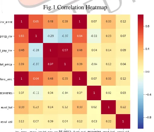
Every Machine Learning model is only as good as the data it is trained with. To ensure optimum and precise predictions, it is essential to train the model on a dataset that is not riddled with redundancies. Data Cleaning refers to the task of purging the data of missing values by either omission or imputation. Columns with more than 50% missing values are dropped. Since the amount of data sacrificed doesn’t explain most of the variance, it won’t affect the predictions. Variables like description of the loan, URL of the website from which the loan was granted, employment title and zip codes are removed since these columns contain an enormous number of categories and will not aid the predictions. Correlation is a statistical measure to assess how a pair of variables are related to each other. A feature correlated with the target variable is important as it aids the predictions. Multi-collinearity increases harmful bias, thereby limiting accuracy. Figure 1 shows the Correlation heatmap for a few features from the dataset.
Fig.1 Correlation Heatmap
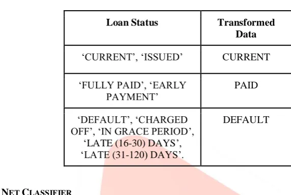
IJEDR1903105 International Journal of Engineering Development and Research (www.ijedr.org) 602 used for dealing with categorical data. Label Encoder basically changes the data type of characters to integers. “Term” is the feature that describes the duration of the loan period, i.e. ‘36 months’ or ‘60 months.’ Similarly, the ‘verification_status’, ‘payment plan’ and ‘application type’ columns are Label Encoded as well. Label Encoding cannot be performed for all categorical features in a dataset. Features with many categories can be treated by grouping them, if they retain their individual properties in a parent group. ‘Loan_status’, ‘homeownership’ and ‘employment length’ are some of the features in which the data is grouped together. Purpose of loan indicates the reason for which the loan request is being issued. It has 13 different categories which are grouped into debt consolidation, educational, small businesses and others. Table 2 indicates how data in the Loan Status column is aggregated.
Table 2
Grouping Status of Loan Column
Loan Status Transformed
Data
‘CURRENT’, ‘ISSUED’ CURRENT
‘FULLY PAID’, ‘EARLY PAYMENT’
PAID
‘DEFAULT’, ‘CHARGED OFF’, ‘IN GRACE PERIOD’,
‘LATE (16-30) DAYS’, ‘LATE (31-120) DAYS’.
DEFAULT
III.DEEP NEURAL NET CLASSIFIER
Neural networks are modelled to function like the human brain. A neural network aims to replicate the cognitive skills which humans possess [4],[5]. Neural networks consist of multiple layers. The layers are made up of neurons, which resemble the ones in the human brain. First, the data is fed to an input layer, which is connected to a single or multiple hidden layer(s) and these hidden layer(s) are connected to the output layer by the means of weights [6]. When the neural net is trained, the weights constantly change in order to fit the training data and minimize training loss.
A Deep Neural Network is essentially a neural network with several hidden layers. Due to its complex architecture and ability to map complex relationships, DNNs are better at pattern recognition, as compared to the traditional machine learning algorithms. Neural networks possess an activation function, a cost function and an Optimizer. Activation Functions are used to determine the output of a neural network. An Optimizer is used to specify, analyze and update the hyperparameters of a neural network in order to generate the best fitting model. The cost function is a metric to evaluate the loss incurred during predictions. The objective is to arrive at a minimum value of loss to achieve accurate predictions. In our research, we have selected the Gradient Descent Algorithm for evaluating cost functions. After applying and comparing the Deep Neural network on various activation functions and optimizers, the minimum amount of loss was obtained when a Rectified Linear Unit (ReLu) activation function [7] was used along with an AdaGrad Optimizer. Adagrad is an optimizer which stresses specifically on parameterized learning rates, which are computed relative to the frequency of updating parameters during training. Higher frequency of updates implies that the update size is smaller [8]. A Deep Neural network classifier is deployed using TensorFlow’s Estimator API in accordance with the above-mentioned parameters. The DNN will use the variables from the dataset as feature vectors and periodically update its weight according to the expected output. The performance of the DNN is evaluated by the Area under ROC Curve. We have also compared the performance of Deep Learning system with traditional Machine Learning algorithms to ascertain if the former performs better than the latter, both in practice and theory.
DNNs have been extensively used for image, audio and video data. However, it’s uses in determining creditworthiness on default loan data has been limited. Our proposed DNN model aims to improve the existing loan disbursal systems and minimizes the cash shortfalls associated with high risk debtors.
IV.IMPLEMENTATION AND OPTIMIZATION
IJEDR1903105 International Journal of Engineering Development and Research (www.ijedr.org) 603 of the model. The report also generates precision, recall and F1-scores for the model. Table V is the classification report for the model before optimization. The DNN achieves an AUC of 60.65%. The DNN performed poorly because the hyperparameters were not fine-tuned to aid the model’s predictions. Table 3 presents the initial results for the unoptimized DNN.
Table 3
Classification Report for Unoptimized DNN
Accuracy 92.43%
Area Under ROC Curve 60.65%
Precision 0.86
Recall 0.92
F1-Score 0.89
Global Steps 5000
Optimization is the process of altering the hyperparameters of the model in order to improve performance and robustness of a system. Optimization is carried out using GridSearchCV, which uses loops to determine the best possible hyperparameters over a wide range of values for number of layers, units in each layer and the number of epochs. Although the process is time consuming, we have observed that it returns the best possible values for tuned hyperparameters.
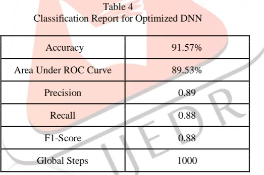
The data split has been changed to 80% for training, 15% for testing and 5% for validation. The number of epochs is increased to 2000 from the original 1000. The number of folds for validation is kept unchanged. The units in the DNN are reduced to 32 per layer. The number of hidden layers is changed to 32. Training is carried over for 1000 steps and the loss is measured every 100 steps. The model not only took lesser time to train but also had a reduced loss. Table 4 shows the report of the optimized Deep Neural Network model.
Table 4
Classification Report for Optimized DNN
Accuracy 91.57%
Area Under ROC Curve 89.53%
Precision 0.89
Recall 0.88
F1-Score 0.88
Global Steps 1000
Although there was a small drop in the accuracy, the optimized DNN has achieved a significantly greater Area under ROC curve. The hyperparameter tuning ensured a reduction in the number of False Positives that were being predicted by the model, thereby augmenting the precision. However, a tradeoff occurs with a drop in the number of false positives. The number of false negatives is observed to increase, thereby decreasing the recall score. Opting for a higher precision implies that the model won’t approve the loan to high risk clients, thereby saving the company a lot of money, which would’ve been lost on a possible Non-Performing Asset (NPA). However, the consequent increase in false negatives implies that a debtor who could be eligible for a loan, won’t be approved by the model. This could adversely affect the approval ratings for the company. The trade-off can be resolved by appropriately deciding if a corporation want’s a higher precision or recall score. In the next section, we discuss why Area under ROC curve has been chosen to evaluate the performance of the model.
V.EVALUATION OF THE MODEL
IJEDR1903105 International Journal of Engineering Development and Research (www.ijedr.org) 604 Table 5
Confusion Matrix
ACTUAL LABELS
0 1
PREDICTED LABELS
0 TRUE
POSITIVE(TP)
FALSE POSITIVE(FP)
1 FALSE
NEGATIVE(FN)
TRUE NEGATIVE(TN)
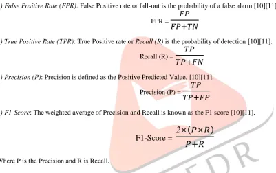
The following statistical parameters are obtained from the confusion matrix:
1) False Positive Rate (FPR): False Positive rate or fall-out is the probability of a false alarm [10][11].
FPR =
𝐹𝑃
𝐹𝑃+𝑇𝑁
2) True Positive Rate (TPR): True Positive rate or Recall (R) is the probability of detection [10][11].
Recall (R) =
𝑇𝑃
𝑇𝑃+𝐹𝑁
3) Precision (P): Precision is defined as the Positive Predicted Value, [10][11].
Precision (P) =
𝑇𝑃
𝑇𝑃+𝐹𝑃
4) F1-Score: The weighted average of Precision and Recall is known as the F1 score [10][11].
F1-Score =
2
×(𝑃×𝑅)
𝑃+𝑅
Where P is the Precision and R is Recall.
The implicit goal of the Area Under Curve (AUC) is to deal with cases in which the target distribution is highly skewed and to avoid overfitting of a single class. Since the target variable that the algorithm will train against is biased towards ‘0’, extremely high accuracy can be achieved if all cases are predicted as ‘0’. Hence, accuracy can be misleading while evaluating a classifier trained on skewed data. Therefore, the AUC is used to evaluate the model.
VI.COMPARATIVE STUDY OF ALGORITHMS
The approach of this paper advocates the use of some traditional Machine Learning algorithms along with a Deep Learning model. Another driving force behind this paper is to observe the performance of Deep Neural Networks on structured data, in the Retail Banking domain. The families of classification algorithms that were selected are Generalized Linear models, Discriminative Classifiers, Ensemble methods [12] and Deep Neural Networks.
Out of the four families of classification algorithms presented in this paper, an algorithm from each category was chosen. Logistic Regression, an algorithm belonging to the generalized linear models [13] is chosen as the baseline model. Apart from the Random Forest Classifier and A Deep Neural Net classifier, a Linear Classifier, belonging to the family of Discriminative Classifiers [14] is also used to forecast credit risk. From the results presented in Table 6, it can be concluded that the Deep Learning model that has been created is best suited for predicting Credit Risk. The model achieves an accuracy of 91.57% and an AUC of 89.53%. Table 6 demonstrates how the algorithms performed in predicting the Credit Risk based on the Area under the ROC.
IJEDR1903105 International Journal of Engineering Development and Research (www.ijedr.org) 605 Performance of Classification Algorithms
Model AUC
Logistic Regression 74.03%
Linear Classifier 71.51%
Random Forest 86.57%
Deep Neural Network 89.53%
VII.CONCLUSION
The Credit Risk Forecasting model was created and trained on a Deep Neural Network model and Lending Club’s data. Based on the results of the classification report, the risk model showed potential to predict Credit Risk precisely.
The ability to analyze, predict and make informed decisions about the implications surrounding Credit Risk will have a widespread influence. If Credit Risk, a measure of the propensity of default can be measured to a high level of precision, creditors will end up making statistically sound decisions. By knowing the credit risk of a debtor, creditors can adjust their lending policies and select their approach towards Credit Risk Management in the light of economic fluctuations and the general instability in the financial markets.
Due to the influence of the Credit Risk model on lending firms, the model needs to be continuously improved. Lending firms need to provide a greater number of data points to train the credit risk model. By providing new features and by researching new machine learning algorithms, the performance of the model can be significantly improved.
Additionally, this model can be used to generate a probability score [0 to 1] to estimate Credit Risk. Automated Lending firms can also use this model to allow debtors to create personal non-collateralized loans and get them approved instantly without having to fill forms or standing in long queues. This greatly improves the customer experience while ensuring the absence of cash shortfalls associated with high default risk.
VIII.ACKNOWLEDGMENT
The authors would like to thank the Department of Data Science at Mahindra & Mahindra Financial Services Limited, headquartered in Mumbai for hosting the research group and allowing access to its resources for the duration of the project. The authors would also like to thank Mr. Rohit Pandharkar, the Head of Data Science for his guidance and consummate tutelage. REFERENCES
[1] K. Y. Tam and M. Kiang, “Managerial Applications of Neural Networks: The Case of Bank Failure Predictions,” Management Science, Vol. 38, No. 7, 1992, pp. 926-947.
[2] T. S. Lee, C. C. Chiu, C. J. Lu and I. F. Chen, “Credit Scoring Using the Hybrid Neural Discriminant Technique”, Expert System with Applications, Vol. 23, No. 3, 2002, pp. 245-254
[3] Z. Huang, H. Chen, C. J. Hsu, W. H. Chen and S. Wu, “Credit Rating Analysis with Support Vector Machines and Neural Networks: A Market Comparative Study,” Decision Support System, Vol. 37, No. 4, 2004, pp. 543-558.
[4] McCulloch, W.S. & Pitts, W. Bulletin of Mathematical Biophysics (1943) 5: 115. https://doi.org/10.1007/BF02478259 [5] Elman, Jeffrey L. (1998). Rethinking Innateness: A Connectionist Perspective on Development. MIT Press. ISBN 978-0-262-55030-7.
[6] Y. Bengio, A. Courville and P. Vincent, "Representation Learning: A Review and New Perspectives," in IEEE Transactions on Pattern Analysis and Machine Intelligence, vol. 35, no. 8, pp. 1798-1828, Aug. 2013.
doi: 10.1109/TPAMI.2013.50
[7] Vinod Nair and Geoffrey E. Hinton. 2010. Rectified linear units improve restricted Boltzmann machines. In Proceedings of the 27th International Conference on International Conference on Machine Learning (ICML'10), Johannes Fürnkranz and Thorsten Joachims (Eds.). Omnipress, USA, 807-814.
[8] Duchi, John; Hazan, Elad; Singer, Yoram (2011). "Adaptive subgradient methods for online learning and stochastic optimization".
IJEDR1903105 International Journal of Engineering Development and Research (www.ijedr.org) 606 [10] Powers, David M W (2011). "Evaluation: From Precision, Recall and F-Measure to ROC, Informedness, Markedness & Correlation" (PDF). Journal of Machine Learning Technologies. 2 (1): 37–63.
[11] Stehman, Stephen V. (1997). "Selecting and interpreting measures of thematic classification accuracy". Remote Sensing of Environment. 62 (1): 77–89. doi:10.1016/S0034-4257(97)00083-7
[12] Opitz, D.; Maclin, R. (1999). "Popular ensemble methods: An empirical study". Journal of Artificial Intelligence Research. [13] Nelder, John; Wedderburn, Robert (1972). "Generalized Linear Models". Journal of the Royal Statistical Society. Series A (General). Blackwell Publishing.