Analysing convergence, consistency and trajectory
of Artificial Bee Colony Algorithm
Jagdish Chand Bansal,
Member, IEEE,
Anshul Gopal and Atulya K. Nagar
Abstract
Recently, swarm intelligence based algorithms gained attention of the researchers due to their wide applicability and ease of implementation. However, much research has been made on the development of swarm intelligence algorithms but theoretical analysis of these algorithms is still a less explored area of the research. Theoretical analyses of trajectory and convergence of potential solutions towards the equilibrium point in the search space can help the researchers to understand the iteration-wise behaviour of the algorithms which can further help in making them efficient. Artificial Bee Colony (ABC) optimization algorithm is swarm intelligence based algorithm. This paper presents the convergence analysis of ABC algorithm using theory of dynamical system. Convergent boundaries for the parameters of ABC update equation have also been proposed. Also the trajectory of potential solutions in the search space is analysed by obtaining a partial differential equation corresponding to the position update equation of ABC algorithm. The analysis reveals that the ABC algorithm performs better when parameters of the update equation are in the convergent region and potential solutions movement follows 1-Dimensional advection equation.
Index Terms
Artificial Bee Colony (ABC) Algorithm, advection equation, convergence analysis, finite difference scheme, swarm intelligence.
I. INTRODUCTION
I
N the recent past, researchers have shown interest in algorithms inspired from natural phenomena. To name a few we have Particle Swarm Optimisation (PSO) algorithm [23] taking inspiration from birds flocking, Artificial Bee Colony (ABC) optimization algorithm [21] inspired by foraging behaviour of honey bees, Gravitational Search Algorithm (GSA) [28] taking inspiration from law of gravity and interaction between the masses, Harmony Search Algorithm (HSA) [12] inspired by improvisation done by jazz musician, Differential Evolution (DE) algorithm [30] inspired by theory of evolution and Spider Monkey Optimization (SMO) [4] algorithm taking inspiration from foraging behaviour of spider monkeys. Recently various variants of ABC algorithm have been proposed which includes modified global best artificial bee colony for constrained optimization problem [3], artificial bee colony algorithm with multiple search strategies [11], an adaptive artificial bee colony algorithm for global optimization [35], hybrid artificial bee colony with differential evolution [18][34], simulated annealing based artificial bee colony algorithm for global numerical optimization [6] and escalated convergent artificial bee colony [17]. Study has shown that these algorithms are considered as an efficient solver of complex optimization problems. Artificial Bee Colony (ABC) optimization algorithm and its variants has been applied to various optimization problems such as solving partition and scheduling problem in codesign [24][14], artificial neural networks [25], forecasting stock markets [15], automatic software fault localization [16], parameter identification for Van Der Pol - Duffing oscillator [10], network topology design [29] and structural engineering [8].Since the inception of ABC algorithm, its different characteristics have been analyzed and investigated, numerically. However, a little work has been done in the theoretical analysis of this class of algorithms.
Jagdish Chand Bansal is with the Department of Mathematics, South Asian University, New Delhi, India, e-mail: ([email protected]). Anshul Gopal is with Department of Mathematics, South Asian University, India and Atulya K. Nagar is with Department of Mathematics and Computer Science, Faculty of Science, Liverpool Hope University, Liverpool, L16 9JD, UK.
Study of stability and convergence behavior of Particle Swarm Optimization (PSO) algorithm is carried out using Z-transformation [19][26][33]. Stability analysis of Differential Evolution (DE) algorithm [7][13], Bacterial Foraging Optimization (BFO) algorithm [5], Ant Colony Optimization (ACO) algorithm [1] and Gravitational Search algorithm (GSA) [9] is done using von Neumann stability criteria and Lyapunov’s stability theorem. Recently, authors’ have performed stability analysis of Artificial Bee Colony (ABC) optimization algorithm using von Neumann stability criteria for two- level finite difference scheme [2]. One of the important aspects is to find the conditions under which the algorithm converges and to study the propagation of potential solutions in the search space using position update equation of the algorithm. Hence, this analysis plays a significant role in the theoretical study of the algorithm. Upto authors’ knowledge no attempt has yet been made for such kind of analysis of ABC algorithm.
In this paper, we investigate the behaviour of ABC algorithm within the convergent boundaries of the parameters. The consistency of finite difference scheme corresponding to position update equation of ABC algorithm with generated partial differential equation is investigated. Trajectory of potential solutions is proposed by investigating the obtained partial differential equation. Then inferences are made by observing the obtained partial differential equation and results obtained from numerical experiments.
Rest of the paper is organized as follows: on the backdrop of original ABC algorithm in Section II, the paper is followed by analysis of trajectory of potential solutions in Section III. Convergence analysis of ABC algorithm is performed in Section IV. Numerical experiments are carried out in Section V, outcomes are discussed in Section VI and findings are concluded in Section VII.
II. ARTIFICIALBEE COLONY(ABC) OPTIMIZATIONALGORITHM
Artificial Bee Colony (ABC) optimization algorithm [21] is a population-based optimization algorithm and makes use of iterative method in order to reach global optima. It consists mainly of four phases. After initialization, exploitation of search space is done employed and onlooker bee phase while exploration is done in scout bee phase. In Artificial Bee Colony (ABC) optimization algorithm employed bees and onlooker bees are present in equal number.
The ABC algorithm has four phases; initialization, employed bee, onlooker bee and scout bee [2].
A. Intialization
Artificial Bee Colony (ABC) optimization algorithm initiates with randomly generated potential solu-tions. For employed bees initial solutions are generated by using the equation:
xi,j =xminj +µ(x
max
j −x
min
j ), i= 1,2, ..N, j = 1,2, ..D (1)
where, xi,j representsjth dimension of theith employed bee.xmaxj is the upper bound andxminj represents
the lower bound of the jth parameter respectively. µ represents uniform random number in the interval
[0,1]. N represents the swarm size and D is the dimension of considered problem. Also, in this phase of the algorithm abandonment counter (AC) is reset for each employed bee.
B. Employeed Bee Phase
A new candidate solution is generated corresponding to each employed bee in this phase. First, the solution of the employed bee is copied to new candidate solution (vi = xi). Then, a randomly selected
parameter ‘j’ of the solution is updated by using the equation:
vi,j =xi,j +φ(xi,j−xr,j) (2)
where i, r ∈
1,2,3..., N , j ∈
1,2,3..., D and i 6= r. xr is randomly selected solution in the
neighbourhood of xi candidate. φ is the random number in [−1,1]. Then fitness of the candidate solution
f iti =
1
1+gi, if fi ≥0
1 +abs(gi), otherwise
where f iti is the fitness value and gi is the value of objective function forith candidate solution. If better
fitness value is achieved then the candidate solution replaces the current solution and the abandonment counter (AC) is reset to zero, otherwise incremented by one.
C. Onlooker Bee Phase
In order to get better solution each employed bee is selected by onlooker bee. The probability for the selection of ith employed bee is calculated by:
pi =
f iti
PN
j=1f itj
(3)
where pi is the probability of selection ofith employed bee. The updation of selected solution is done by
using equation (2). Again if better fitness is achieved then employed bee is replaced with onlooker bee and AC is reset to zero. Otherwise AC is increased by unity.
D. Scout Bee Phase
In this phase AC of all potential solutions are checked for predefined limit.Those employed bees whose AC has reached the predefined limit becomes scout bee. Thereafter for scout bees the solution is generated by using equation (1) and AC is set to zero. The scout bee then becomes employed bee and hence prevents stagnation of the algorithm.
III. TRAJECTORY OF POTENTIAL SOLUTIONS INARTIFICIALBEE COLONY(ABC)ALGORITHM
A. Motivation
Nature inspired optimization algorithms are used to solve real-world optimization problems. It is not always necessary that the potential solutions converge to equilibrium point as the iteration increases, they may diverge from the desired equilibrium point.Therefore it is important to study the conditions under which the potential solutions and hence the ABC algorithm converge to the desired equilibrium point. φ and ψ are two parameters used in the position update equation of ABC algorithm. The study of convergence will provide necessary recommendations for parameter setting of the parameters φ and
ψ. Also, it is necessary to understand how the solutions move near optimal solution in the search space. This motivates the authors to study the iteration-wise movement of solutions, which are updated using position update equation (2) of the ABC algorithm. Convergent region is defined as the region bounded by parameters φ and ψ, where the algorithm converges to equilibrium point.
B. Partial Differential Equation associated with position update equation of ABC algorithm
In this section, we generate initial value problem associated with position update equation of ABC algorithm with the help of finite difference scheme corresponding to position update equation given in equation (2).
vi,j =xi,j +φ(xi,j−xr,j)
where i, r ∈
1,2,3..., N ; j ∈
1,2,3..., D and i 6= r. If t represents the present iteration and the
solution got updated, then xi,j represents the solution at iteration t and vi,j represents the solution at
iteration (t+ 1). So the above equation can be written as [2]:
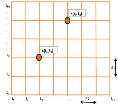
Fig. 1: Grid point representation of approximate solutions.
In ABC algorithm, the position update equation (4) is implemented component wise, i.e. the dimension of a solution is updated independently. The only link between the dimensions of the problem space is introduced via objective function. Thus, without loss of generality, for analysis purpose the algorithm description can be reduced to the one dimension case as considered in [33][9][7]. Thus equation (4) can be written as:
xi(t+ 1)−xi(t) =φ(xi(t)−xr(t)) (5)
where, r is randomly selected solution index different from i. If x = x(i, t) represents true solution to a problem in an i-t computational domain. Then, xl,n =x(il, tn) represents the approximate solution on
the nodes of a uniform computational grid such that ∆i=∆t, l ∈
1,2,3..., b1 and n ∈
1,2,3..., b2 ,
where ∆i and ∆t are grid spacing in the direction of i and t respectively (shown in Figure 1).
In terms of grid points the difference equation can further be written as:
x(il, tn+1)−x(il, tn) = φ(x(il, tn)−x(ir, tn)); x(il,1) = g(il) (6)
where, l, r ∈
1,2,3..., b1 and n∈
1,2,3..., b2 .
Since l, r∈
1,2,3..., b1 , we can write r=l+a where, a∈Z/
0 such that r∈
1,2,3..., b1 .
The above equation (6) can now be written as:
x(il, tn+1)−x(il, tn) =φ(x(il, tn)−x(il+a, tn)); x(il,1) =g(il) (7)
As discussed earlier since we have considered uniform grid for our analysis, so the grid spacings are of equal length i.e. ∆t = ∆i. Hence, equation (7) can be written as:
x(il, tn+1)−x(il, tn)
∆t =
φ(x(il, tn)−x(il+a, tn))
∆i ; (8)
x(il,1) = g(il)
Since a∈Z/
0 , so the above equation (8) can be written as:
x(il, tn+1)−x(il, tn)
∆t =
aφ(x(il, tn)−x(il+a, tn))
x1
l =x(il,1) =g(il)
or
xnl+1−xn
l ∆t =
aφ(xnl −xnl+a)
a∆i ; (10)
x1
l =x(il,1) = g(il)
where, xn
l = x(il, tn). The partial differential equation corresponding to above difference equation and
hence corresponding to position update equation of ABC algorithm with initial condition is given by:
∂x
∂t =−aφ
∂x
∂i; x(i,1) = g(i) (11)
or
∂x
∂t +v
∂x
∂i = 0; x(i,1) = g(i) (12)
where, ∂x∂t = x(il,tn+1)−x(il,tn)
∆t , ∂x
∂i =
(x(il+a,tn)−x(il,tn))
a∆i , v= aφ and x is the exact solution of the partial
differential equation (12).
By analyzing equation (12) we can infer that the partial differential equation corresponding to position update equation of ABC algorithm resembles 1- Dimension advection equation [20].
In the next subsection, we will verify that the difference scheme corresponding to position update equation of ABC algorithm given in equation (10) is consistent with the partial differential equation obtained in equation (12).
C. Consistency
Definition:[32] Let the partial differential equation under consideration be denoted by Ly=F and the
corresponding finite difference approximation by Lnlxnl =Gnl, where Gnl denotes whatever approximation has been made of the source term. If we write the difference scheme as:
xnl+1 =Qxnl + ∆tGnl (13)
where, xn
l = (..., xn−1, x0n, xn1...)T, Gln = (..., Gn−1, Gn0, Gn1...)T and Q is an operator acting on the
ap-propriate space. The difference scheme (13) is pointwise consistent with the partial differential equation
(Ly=F) if the solution of the partial differential equation, y, satisfies
yln+1 =Qynl + ∆tGnl + ∆tτln (14)
and τln →0 as ∆i,∆t→0. We refer to τln as truncation error.
To show that the difference scheme (10) is consistent, we must write the scheme in the form of equation (13) as:
xnl+1 =xnl +φa∆t
a∆i(x
n
l −xnl+a) (15)
Equation (15) gives each component of an equation in the form of (13). Hence, to apply definition of consistency, we let x to be a solution of partial differential equation (12) and write:
∆tτln =xnl+1−[xnl +φa∆t
a∆i(x
n l −x
n
l+a)] (16)
By expanding the components with the help of Taylor series we get:
∆tτln=hxnl + (xt)nl∆t+ (xtt)nl ∆t2
2 +....
i −
n
xnl +φa∆t
a∆i
h
xnl −xnl + (xi)nla∆i+ (xii)nl
(a∆i)2 2 −..
With proper rearrangement and cancellation of components in the above equation (17) we get:
∆tτln = (xt)nl∆t+aφ(xi)nl∆t+ (xtt)nl ∆t2
2 +φ(xii) n l
a2∆t∆i
2 +... (18)
By dividing both sides of equation (18) by ∆t, we get the required equation as:
τln = (xt+aφxi)nl + (xtt)nl
∆t
2 +φ(xii) n l
a2∆i
2 +... (19)
or
τln= (xt+vxi)nl + (xtt)nl
∆t
2 +φ(xii) n l
a2∆i
2 +... (20)
Using equation (12) the above equation is modified to get the value of τn l as:
τln= (xtt)nl ∆t
2 +φ(xii) n l
a2∆i
2 +... (21)
or
τln =o(∆t) +o(∆i) (22)
According to the definition of consistency discussed previously, τn
l →0 as ∆i,∆t →0. Also, under the
assumption that higher order derivatives of xare bounded at (l∆i, n∆t)the considered difference scheme has accuracy of order (1,1).
Hence, the finite difference scheme given by equation (10) corresponding to position update equation of ABC algorithm is consistent with the obtained partial differential equation given by equation (12). In the next section, numerical experiments are done for deterministic analysis of the findings.
D. Lax Equivalence Theorem
Definition:A consistent, two level finite difference scheme for a well posed linear initial value problem
is convergent iff it is stable [32].
Authors have already proved stability of position update equation of ABC algorithm in [2]. Also, con-sistency of the position update equation is proved in section 3.3. Since the corresponding initial value problem depends continuously upon its initial conditions, it is well posed too. Therefore by Lax equivalence theorem considered difference scheme corresponding to position update equation of ABC algorithm is convergent to the obtained partial differential equation given by equation (12).
Physical meaning of convergence:
∆t → 0 indicates that distance between grid points in the direction of t tends to zero i.e., number of iterations reaches to maximum limit. While ∆i → 0 implies that, distance between grid points in the direction of i tends to zero i.e., distance between particles tend to zero, which means particles are getting clustered at a particular location in the search space.
These two inferences imply that when particles get clustered in the search space as number of iterations reaches to maximum limit, then the solutions obtained from difference equation (5) coincides with the solutions obtained from partial differential equation (12).
IV. CONVERGENCEANALYSIS OFABC ALGORITHM
In this section, the conditions under which the potential solutions considered in ABC algorithm con-verges to an equilibrium point is obtained. In order to do so, we first introduce a parameterψ(as coefficient) in the position update equation of ABC algorithm.
vi,j =ψxi,j+φ(xi,j−xr,j), (23)
where i, r ∈
1,2,3..., N , j ∈
1,2,3..., D and i 6= r. All the parameters are same as defined in
III, without loss of generality for analysis purpose the algorithm description can be reduced to one dimension case as considered in [33][9][7]. Thus equation (23) can be written as (as done in section ??)
xi(t+ 1) =ψxi(t) + φ(xi(t)−xr(t)) (24)
or
xi(t+ 1) = (ψ+φ)xi(t) − φxr(t) (25)
For theoretical analysis of ABC algorithm, the deterministic version of position update equation is considered. Deterministic version is obtained by replacing random entity with the expected value. In equation (25), xr is the position of randomly selected candidate solution in the neighbourhood of xi. So,
in order to obtain deterministic version of position update equation of ABC algorithm, we have to replace the position of randomly selected candidate solution by any expected value say ‘p’, i.e. xr = p. Now
equation (25) can be written as
xi(t+ 1) = (ψ+φ)xi(t) − φp (26)
The dynamic behaviour of potential solutions in the search space can be analysed by using the study of linear discrete-time dynamical system [33]. Equation (26) can be written in matrix form as
Yt+1 =AYt+Bp (27)
where, Yt = [xi(t)]1∗1, A= [ψ+φ]1∗1 and B = [−φ]1∗1
In accordance with the theory of dynamical systems, Yt represents the particle state, comprising of its
current positionxi(t). The properties of dynamic matrix ‘A’ determines the time behaviour of the particle.
External input ‘p’ helps in moving the particle towards specified position while input matrix ‘B’ provides the effect of external input on the particle state.
A. Equilibrium point
Definition: An equilibrium point is a state maintained by the dynamical system in the absence of
external excitation (i.e., p= constant) [33].
If any equilibrium point exists then it satisfies the condition
Yteq+1 =Yteq; ∀ t (28)
By using the above condition in equation (26), the equilibrium point is calculated as:
xeqi = −φp
1−ψ−φ (29)
Without loss of generality, equation (23) can also be simplified and written as
xi(t+ 1) =ψxi(t) + φ(xr(t)−xi(t)) (30)
or
xi(t+ 1) = (ψ−φ)xi(t) + φxr(t) (31)
or
xi(t+ 1) = (ψ−φ)xi(t) + φp (32)
So, the corresponding equilibrium point is given by:
xeqi = φp
1−ψ +φ (33)
For ψ = 1 i.e. in case of original ABC algorithm, the equilibrium point is calculated asxeqi =p for both the cases.
It can be clearly observed that in the presence of coefficient ψ, the equilibrium point depends upon both parameters ψ and φ, whereas when coefficient ψ = 1 the equilibrium point is independent of both the parameters. Hence we can say that with the introduction of coefficient ψ (ψ 6= 1), the role of parameter
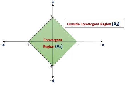
Fig. 2: Convergence boundary for parameters ψ and φ.
B. Convergence
In general, initially the particle state is not at equilibrium. So it is necessary to analyse whether the particle will eventually move towards equilibrium or not i.e., the optimization algorithm will converge or not. From the results of theory of dynamical system it can be concluded that the eigenvalues of the dynamic matrixA plays an important role in explaining the time behaviour of the potential solutions [22]. The necessary and sufficient condition for equilibrium point to be stable is that the magnitude of eigen values of the matrix A should be less than unity [33]. In this case the potential solutions will eventually settle at equilibrium and the algorithm will converge. By using equation (27), the matrix A has only one eigen value given by λ1 =ψ+φ. As discussed above for the convergence of ABC algorithm
|λ1|<1 i.e. |ψ+φ|<1 (34)
Without loss of generality, equation (23) can also be written as:
xi(t+ 1) =ψxi(t) + φ(xr(t)−xi(t)) (35)
or
xi(t+ 1) = (ψ−φ)xi(t) + φxr(t) (36)
The corresponding eigen value will be given by λ2 =ψ−φ and hence the condition for convergence of
ABC algorithm will be given by:
|λ2|<1 i.e. |ψ−φ|<1 (37)
By combining results from equation (34) and (37) the condition for convergence of ABC algorithm with coefficient ψ is:
|ψ+φ|<1 and |ψ−φ|<1 (38)
The convergence boundary for the parameters ψ and φ is shown in Figure 2. In Figure 2, the shaded region (A1) is termed as convergent region and (A2) as outside convergent region. Convergent region
signifies that, if the values of parameters φ and ψ lie within region (A1) then the potential solutions will
TABLE I: List of Test Problems (AE: Acceptable Error, U: Uni-modal, M: Multi-modal, S: Separable,
N: Non-separable ) [27] [31]
Name of the problem Search
Range Optimum Value Dim(n) AE Characteristic
Ackley [−30,30] f(~0) = 0 30 1.0E−05 M, S
Alpine [−10,10] f(~0) = 0 30 1.0E−05 M, S
Salomon [−100,100] f(~0) = 0 30 2.0E−01 M, N
Pathological [−100,100] f(~0) = 0 30 1.05E−01 M, N
Inverted Cosine wave [−5,5] f(~0) =−n+ 1 10 1.0E−05 M, S
Shifted Rosenbrock [−100,100] f(o) = f(~0) =
390 10 1.0E
−01 M, N
De Jong [−5.12,5.12] f(~0) = 0 30 1.0E−05 U, S
Moved axis parallel hyper-ellipsoid [−5.12,5.12] f(~0) = 0 30 1.0E−15 U, S
Shifted Rotated and expanded uneven
minima [
−100,100] f(~0) = 500 30 1913.0 M, N
Composition function 3 [−100,100] f(~0) = 1100 30 325.0 M, N
V. NUMERICAL EXPERIMENT
In order to justify our theoretical findings for convergence analysis of ABC algorithm, numerical testing is carried out on a set of 10 benchmark problems. The benchmark problems considered have objective function with properties which includes unimodal, multimodal, separable and non-separable functions. In addition to that few have optimal point at origin and others have optimal point away from origin as explained in Table I. While doing numerical experiments to verify the findings of convergence analysis, two cases are considered. Firstly, when parameters φ and ψ lie within convergence region and secondly when they lie outside convergence region.
Following three types of numerical experiments are performed:
1) In subsection (V-A), movement of potential solution in the search space is analysed.
2) In subsection (V-B), efficiency of the algorithm is tested by calculating average number of function evaluations.
3) In subsection (V-C), accuracy of the algorithm is checked by analysing the mean error of considered test problems.
A. Movement of potential solution in the search space
In order to justify our finding that movement of solutions in ABC algorithm follows advection equation, numerical analysis is done with usual parameter settings. The general solution of the partial differential equation (11) can be written as [Appendix A]:
x(i, t) =g(i−aφ(t−1)) (39)
While, the position update equation of ABC algorithm along with initial solution xi(1) is given by:
xi(t+ 1) =xi(t) + φ(xi(t)−xr(t)); xi(1) =g(i) (40)
Following parameter settings are considered for the numerical experiment:
1 2 3 4 5 6 7 8 9 10 −1
−0.8 −0.6 −0.4 −0.2 0 0.2 0.4 0.6 0.8 1
Iterations
Particle Position
Solution of PDE Solution by ABC update equation
Fig. 3: Positions of solutions obtained from ABC update equation and solution of PDE.
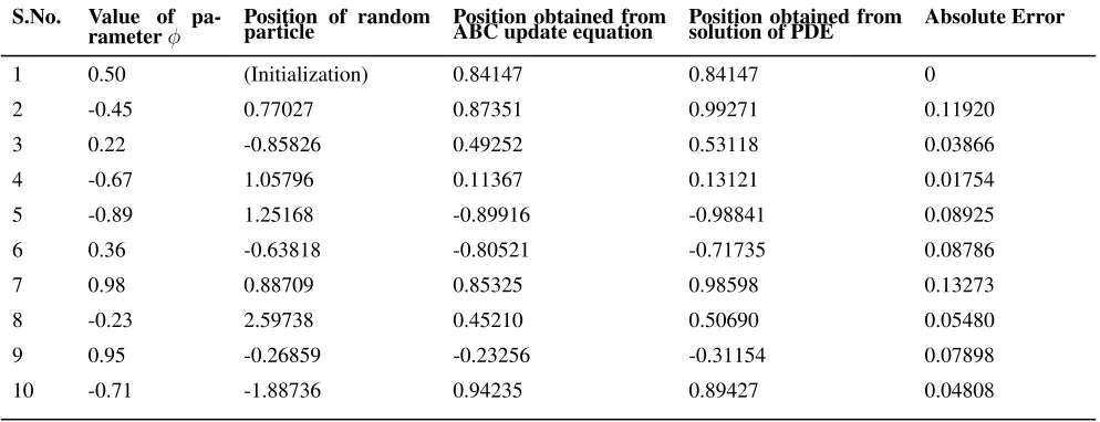
TABLE II: Comparision of numerical results with random initialization (i.e., g(i) = 0.84147)” (PDE:
Partial differential equation)
S.No. Value of
pa-rameterφ Position of randomparticle Position obtained fromABC update equation Position obtained fromsolution of PDE Absolute Error
1 0.50 (Initialization) 0.84147 0.84147 0
2 -0.45 0.77027 0.87351 0.99271 0.11920
3 0.22 -0.85826 0.49252 0.53118 0.03866
4 -0.67 1.05796 0.11367 0.13121 0.01754
5 -0.89 1.25168 -0.89916 -0.98841 0.08925
6 0.36 -0.63818 -0.80521 -0.71735 0.08786
7 0.98 0.88709 0.85325 0.98598 0.13273
8 -0.23 2.59738 0.45210 0.50690 0.05480
9 0.95 -0.26859 -0.23256 -0.31154 0.07898
10 -0.71 -1.88736 0.94235 0.89427 0.04808
2) Since we are performing numerical analysis and swarm size is fixed to two solutions, so the random solution index (r) will be taken as r = 2, (r6=i ).
3) In order to follow the phenomena of exploration and exploitation, some random values of parameter
φ are considered in the range [-1, 1], given in Table II.
4) The concept of greedy selection is used while choosing the position of a random solution in the neighbourhood of the candidate solution.
5) Initialization function g(i) is selected randomly (given in Table II) for performing the numerical analysis.
Now we will compare the numerical results obtained by solving equation (39) and (40), simultaneously the outcome of the numerical results is listed in Table II and shown graphically in Figure 3.
B. Efficiency of the algorithm
In order to check the efficiency of ABC algorithm, numerical experiments are performed when param-eters are considered within and outside convergent region. Following parameter settings are considered while doing the numerical experiment.
1) Swarm size: 50
2) Maximum number of runs: 51
3) Maximum number of iterations: 6000 4) Acceptable error: Table I
The average number of function evaluations (AFEs) are calculated and reported in Table III for both the cases, i.e. when parameters lie within the convergent region A1 (as shown in Figure 2) and outside
TABLE III: Average number of Function Evaluations (AFEs) for region A1 andA2 (see Figure 2) (TP:
Test Problem, A1: Parameters within convergence region, A2: Parameters outside convergence region)
TP AFEs forA1 AFEs forA2
f1 22698 198610
f2 27900 200026
f3 198305 200030
f4 156353 200028
f5 14538 199371
f6 75 75
f7 5022 27805
f8 28573 200025
f9 261833 300050
f10 168729 299221
Parameters Within Convergent Region Parameters Outside Convergent Region −0.5
0 0.5 1 1.5 2 2.5 3
x 105
Average No. Of function Evaluations
Fig. 4: Boxplot comparison of AFEs for regionA1 andA2 (A1: Parameters within convergent region,A2:
Parameters outside convergent region).
or maximum number of function evaluation is attained whichever is earlier. From the experimental results it is clear that ABC algorithm is efficient when parameters lie within A1. The difference of results when
parameters lie in A1 and A2 can be seen from the boxplot shown in Figure 4.
C. Accuracy of the algorithm
To check the accuracy of ABC algorithm, numerical experiments have been carried out by considering parameters within and outside convergent region. Parameter setting and test problems are same as con-sidered in section V-B. Mean Error (ME) is calculated for concon-sidered test problems and numerical results are presented in Table IV. The improvement of accuracy of ABC algorithm with parameters within region
A1 and A2 can be observed from the boxplot shown in Figure 5. Numerical results are again verified
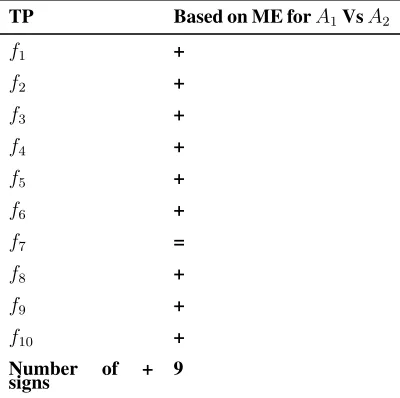
by performing non parametric test namely, Wilcoxon signed rank test and presented in Table V. If the obtained data sets have significant difference then we say that null hypothesis is rejected and ‘+’ sign appears otherwise null hypothesis is accepted and ‘=’ sign appears. In Table V, ‘+’ sign appears 9 times out of 10. Thus the accuracy of ABC algorithm is better when parameters φ and ψ are considered in convergent region A1.
VI. DISCUSSION
TABLE IV: Mean Error (ME) for regionA1 andA2 (TP: Test Problem,A1: Parameters within convergent
region, A2: Parameters outside convergent region)
TP ME forA1 ME forA2
f1 8.42E-06 2.72E-05
f2 7.48E-06 0.127836
f3 0.57 1.61
f4 0.097 13.837
f5 6.17E-06 0.348546
f6 8.32E05 1.04E06
f7 4.47E-06 4.72E-06
f8 8.6E-16 2.04E-13
f9 2117.71 2509.26
f10 325.47 360.76
Parameters Within Convergent Region Parameters Outside Convergent Region −30
−20 −10 0 10
Logarithm of Mean Error
Fig. 5: Boxplot comparison of ME for region A1 and A2 (A1: Parameters within convergent region, A2:
Parameters outside convergent region).
TABLE V: Comparision of Mean Error (ME) for region A1 and A2 using Wilcoxon Sign Rank test(TP:
Test Problem, A1: Parameters within convergent region, A2: Parameters outside convergent region)
TP Based on ME forA1VsA2
f1 +
f2 +
f3 +
f4 +
f5 +
f6 +
f7 =
f8 +
f9 +
f10 +
Number of +
section IV. From the numerical experiments (Table III) it can be easily seen that the AFEs are minimum for test problems in convergent region which shows that the test problems are converging towards equilibrium point in less number of iterations when parameters are in the convergent region. Results are further verified statistically by boxplot analysis of AFEs and ME. Again it can be seen that better results are obtained when parameters are within convergent region. The mean error for test problems in convergent region is also minimum as compared to the case when parameters lie outside convergent region which shows that the accuracy is better within convergent region. The results are verified by non parametric test, namely wilcoxon signed rank test. It can be inferred that result are significantly better when parameters are within convergent region.
Also, theoretical and numerical analyses of ABC position update equation reveals that the difference scheme (10) corresponding to position update equation (III-B) of ABC algorithm is consistent with the partial differential equation (12). The obtained partial differential equation infact resembles 1-Dimensional advection equation. The general solution of the partial differential equation obtained in equation (12) is given by x(i, t)=f(i−vt). Where ‘f’ is an arbitrary function depending upon the initial condition and
v= aφ. The solution obtained describes an arbitrary shaped pulse which is swept along by the flow at constant speed ‘v’ without changing shape. Since a ∈ Z/0 and φ ∈ [−1,1], speed ‘v’ can be either positive or negative. Hence, the arbitrary shaped pulse generated can move in either forward direction or backward which explains that ABC algorithm can explore the entire search space. The analysis also explains a significant result that the propagation of particles depends upon the initial condition, i.e. the initialization phase of ABC algorithm plays an important role in the movement of solutions in the search space.
VII. CONCLUSION
Analysis of finding the conditions under which an algorithm converges to an equilibrium point plays a very vital role in making the algorithm efficient, reliable and accurate. For nature inspired algorithms, the solution update process depends upon the guided random search, which makes algorithm’s nature probabilistic. This probabilistic nature of these algorithms makes the convergence analysis a difficult task. Convergence analysis of ABC algorithm is performed using the results from the theory of dynamical systems. Also condition of convergence of algorithm to equilibrium point is derived, which depends upon the parameters φ and ψ. Numerical experiments are performed to verify the findings and a convergent region is recommended for the values of φ and ψ. It can be concluded that the algorithm performs better when parameters are considered from the convergent region.
Also, study of the movement of solutions in the search space is important to analyse the search behaviour of ABC algorithm. In order to carry out this study, partial differential equation associated with position update equation of ABC algorithm is obtained. The obtained partial differential equation resembles 1-Dimensional advection equation. It was also proved that the finite difference scheme corresponding to position update equation of ABC algorithm is consistent with the obtained partial differential equation. So, from the general solution of the partial differential equation, it can be concluded that the solutions obtained by ABC algorithm propagate in an arbitrary shaped pulse which is swept along the flow at constant speed without changing shape.
ACKNOWLEDGMENT
The second author acknowledges the funding from South Asian University New Delhi, India to carry out this research.
APPENDIXA
GENERAL SOLUTION OFPDE
The general solution of partial differential equation (12) is given by:
TABLE VI: List of Test Problems considered for numerical experiments [27] [31]
Name of the problem Objective function
Ackley M inf1(x) =−20 +e+exp(−0n.2pPni=1xi3)
Alpine M inf2(x) =
Pn
i=1|xisinxi+ (0.1)xi|
Salomon M inf3(x) = 1−cos(2π
pPn
i=1x2i) + 0.1(
pPn i=1x2i)
Pathological M inf4(x) =
Pn−1 i=1
sin2(√x2
i+1+100x2i)−0.5
0.001(x2
i+1−2xi+1xi+x2i)2+1.0 + 0.5
Inverted Cosine wave M inf5(x) =−
Pn−1
i=1
exp
−(x2
i+x2i+1+0.5xixi+1)
8
×i
Shifted Rosenbrock M inf6(x) =
Pn−1
i=1(100(zi2−zi+1)2+ (zi−1)2) +fbias,z =
x−o+ 1,x= [x1, x2, ....xn],o= [o1, o2, ...on]
De Jong M inf7(x) =
Pn i=1i.(xi)
4
Moved axis parallel hyper-ellipsoid M inf8(x) =
Pn
i=15i×x 2
i
Shifted Rotated and expanded uneven
minima M inf9(x) = (CEC2015) Composition function 3 M inf10(x) = (CEC2015)
with initial condition given as:
x(1, t) = g(i) (42)
By using equation (43) and (44) we get
x(1, t) =f(i−aφ) =g(i) (43)
or
f(I) =g(I+aφ), where I =i−aφ (44)
By using equation (41) and (44) we get the final solution of partial differential equation as
x(i, t) = g(i−aφt+aφ) (45)
or
x(i, t) =g(i−aφ(t−1)) (46)
REFERENCES
[1] Ajith Abraham, Amit Konar, Nayan R Samal, and Swagatam Das. Stability analysis of the ant system dynamics with non-uniform pheromone deposition rules. In Evolutionary Computation, 2007. CEC 2007. IEEE Congress on, pages 1103–1108. IEEE, 2007.
[2] Jagdish Chand Bansal, Anshul Gopal, and Atulya K Nagar. Stability analysis of artificial bee colony optimization algorithm. Swarm and Evolutionary Computation, 2018.
[3] Jagdish Chand Bansal, Susheel Kumar Joshi, and Harish Sharma. Modified global best artificial bee colony for constrained optimization problems. Computers & Electrical Engineering, 2017.
[4] Jagdish Chand Bansal, Harish Sharma, Shimpi Singh Jadon, and Maurice Clerc. Spider monkey optimization algorithm for numerical optimization. Memetic computing, 6(1):31–47, 2014.
[5] Arijit Biswas, Swagatam Das, Ajith Abraham, and Sambarta Dasgupta. Stability analysis of the reproduction operator in bacterial foraging optimization. Theoretical Computer Science, 411(21):2127–2139, 2010.
[7] Sambarta Dasgupta, Swagatam Das, Arijit Biswas, and Ajith Abraham. On stability and convergence of the population-dynamics in differential evolution. Ai Communications, 22(1):1–20, 2009.
[8] ZH Ding, M Huang, and ZR Lu. Structural damage detection using artificial bee colony algorithm with hybrid search strategy. Swarm and Evolutionary Computation, 28:1–13, 2016.
[9] Faezeh Farivar and Mahdi Aliyari Shoorehdeli. Stability analysis of particle dynamics in gravitational search optimization algorithm. Information Sciences, 337:25–43, 2016.
[10] Fei Gao, Xue-jing Lee, Feng-xia Fei, Heng-qing Tong, Yi-bo Qi, Yan-fang Deng, Ilangko Bal-asingham, and Hua-ling Zhao. Parameter identification for van der pol–duffing oscillator by a novel artificial bee colony algorithm with differential evolution operators. Applied Mathematics and Computation, 222:132–144, 2013.
[11] Wei-feng Gao, Ling-ling Huang, San-yang Liu, Felix TS Chan, Cai Dai, and Xian Shan. Artificial bee colony algorithm with multiple search strategies. Applied Mathematics and Computation, 271:269– 287, 2015.
[12] Zong Woo Geem, Joong Hoon Kim, and GV Loganathan. A new heuristic optimization algorithm: harmony search. Simulation, 76(2):60–68, 2001.
[13] Anshul Gopal and Jagdish Chand Bansal. Stability analysis of differential evolution. In Computa-tional Intelligence (IWCI), InternaComputa-tional Workshop on, pages 221–223. IEEE, 2016.
[14] Shih-Cheng Horng. Combining artificial bee colony with ordinal optimization for stochastic economic lot scheduling problem. IEEE Trans. Systems, Man, and Cybernetics: Systems, 45(3):373–384, 2015. [15] Tsung-Jung Hsieh, Hsiao-Fen Hsiao, and Wei-Chang Yeh. Forecasting stock markets using wavelet transforms and recurrent neural networks: An integrated system based on artificial bee colony algorithm. Applied soft computing, 11(2):2510–2525, 2011.
[16] Linzhi Huang and Jun Ai. Automatic software fault localization based on artificial bee colony.
Journal of Systems Engineering and Electronics, 26(6):1325–1332, 2015.
[17] Shimpi Singh Jadon, Jagdish Chand Bansal, and Ritu Tiwari. Escalated convergent artificial bee colony. Journal of Experimental & Theoretical Artificial Intelligence, 28(1-2):181–200, 2016. [18] Shimpi Singh Jadon, Ritu Tiwari, Harish Sharma, and Jagdish Chand Bansal. Hybrid artificial bee
colony algorithm with differential evolution. Applied Soft Computing, 58:11–24, 2017.
[19] Visakan Kadirkamanathan, Kirusnapillai Selvarajah, and Peter J Fleming. Stability analysis of the particle dynamics in particle swarm optimizer. IEEE Transactions on Evolutionary Computation, 10(3):245–255, 2006.
[20] Takeo Kajishima and Kunihiko Taira. Finite-difference discretization of the advection-diffusion equation. In Computational Fluid Dynamics, pages 23–72. Springer, 2017.
[21] Dervis Karaboga. An idea based on honey bee swarm for numerical optimization. Technical report, Technical report-tr06, Erciyes university, engineering faculty, computer engineering department, 2005.
[22] Anatole Katok and Boris Hasselblatt. Introduction to the modern theory of dynamical systems, volume 54. Cambridge university press, 1995.
[23] James Kennedy. Particle swarm optimization. In Encyclopedia of machine learning, pages 760–766. Springer, 2011.
[24] Mouloud Koudil, Karima Benatchba, Amina Tarabet, and El Batoul Sahraoui. Using artificial bees to solve partitioning and scheduling problems in codesign. Applied Mathematics and Computation, 186(2):1710–1722, 2007.
[25] Pravin Yallappa Kumbhar and Shoba Krishnan. Use of artificial bee colony (abc) algorithm in artificial neural network synthesis. International Journal of Advanced Engineering Sciences and Technologies, 11(1):162–171, 2011.
[26] Ning Li, De-Bao Sun, Tong Zou, Yuan-Qing Qin, and Yu Wei. Analysis for a particle’s trajectory of pso based on difference equation. Jisuanji Xuebao/Chinese Journal of Computers, 29(11):2052–2061, 2006.
the cec 2015 competition on single objective multi-niche optimization. Computational Intelligence Laboratory, Zhengzhou University, Zhengzhou, China, Tech. Rep., 2014.
[28] Esmat Rashedi, Hossein Nezamabadi-Pour, and Saeid Saryazdi. Gsa: a gravitational search algorithm.
Information sciences, 179(13):2232–2248, 2009.
[29] Amani Saad, Salman A Khan, and Amjad Mahmood. A multi-objective evolutionary artificial bee colony algorithm for optimizing network topology design. Swarm and Evolutionary Computation, 38:187–201, 2018.
[30] Rainer Storn and Kenneth Price. Differential evolution–a simple and efficient heuristic for global optimization over continuous spaces. Journal of global optimization, 11(4):341–359, 1997.
[31] Ponnuthurai N Suganthan, Nikolaus Hansen, Jing J Liang, Kalyanmoy Deb, Ying-Ping Chen, Anne Auger, and Santosh Tiwari. Problem definitions and evaluation criteria for the cec 2005 special session on real-parameter optimization. KanGAL report, 2005005:2005, 2005.
[32] James William Thomas. Numerical partial differential equations: finite difference methods, vol-ume 22. Springer Science & Business Media, 2013.
[33] Ioan Cristian Trelea. The particle swarm optimization algorithm: convergence analysis and parameter selection. Information processing letters, 85(6):317–325, 2003.
[34] Jing Yang, Wen-Tao Li, Xiao-Wei Shi, Li Xin, and Jian-Feng Yu. A hybrid abc-de algorithm and its application for time-modulated arrays pattern synthesis. IEEE Transactions on Antennas and Propagation, 61(11):5485–5495, 2013.
[35] Alkın Yurtkuran and Erdal Emel. An adaptive artificial bee colony algorithm for global optimization.
Applied Mathematics and Computation, 271:1004–1023, 2015.
Jagdish Chand Bansal has recieved his Ph.D. from Indian Institute of Technology Roorkee, India. He is currently an Assistant Professor at South Asian University, New Delhi, India and Visiting Research Fellow at Liverpool Hope University, UK. He is the editor-in-chief of International Journal of Swarm Intelligence (IJSI) published by Inderscience. He is also the editor-in-chief of Springer book series Algorithms for Intelligent Systems. His primary area of interest is nature-inspired optimization techniques.
Anshul Gopal received his M.Sc. degree in Mathematics from University of Delhi, New Delhi, India in 2011. Currently, he is perusing Ph.D. from South Asian University, New Delhi, India. His area of research is nature-inspired optimization algorithms and soft computing.
![TABLE I: List of Test Problems (AE: Acceptable Error, U: Uni-modal, M: Multi-modal, S: Separable,N: Non-separable ) [27] [31]](https://thumb-us.123doks.com/thumbv2/123dok_us/1086188.1609253/9.612.79.548.85.301/table-list-problems-acceptable-error-multi-separable-separable.webp)

![TABLE VI: List of Test Problems considered for numerical experiments [27] [31]](https://thumb-us.123doks.com/thumbv2/123dok_us/1086188.1609253/14.612.88.533.73.282/table-vi-list-test-problems-considered-numerical-experiments.webp)
