A Performance Prediction Method for Pumps as Turbines (PAT) Using a CFD Modeling Approach

Generators, International Journal of Engineering (IJE), TRANSACTIONS B: Applications Vol. Also, the results of lift and drag coefficients were validated using experimental data.

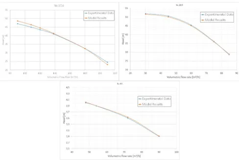
The contribution of the present paper is to extend this scheme and apply it to new cases for which the results are compared against available experimental data and other

Inspection data are available since the 1992 for all major bridge elements, creating a 25-year database for analysis and modeling. In the pilot study described in this paper,

These include the visualization algorithm for the generation of the treemap models based on the procedure data, various analysis algorithms to query the mutual influence of

The Hybrid LES/RANS results are compared with RANS as well as a variety of experimental and diagnostic data including hydroxyl planar laser-induced fluorescence (OH-PLIF),

To verify the proposed multiscale framework, predictions obtained via the proposed model are compared with experimental data and results estimated by the previous work, which show

[17] used the data to simulate the response of the nanoDot OSL dosimeter using a megavoltage photon beam and they compared with experimental results; although the data

The audiovisual feature is used to classify the data into corresponding emotion using PCA-BFO method.. Experimental results demonstrate the effectiveness of the