Article
Mutual Information, the Linear Prediction Model,
and CELP Voice Codecs
Jerry Gibson
1
2
3
4
5
6
7
8
9
10
11
1 DepartmentofElectricalandComputerEngineering,UniversityofCalifornia,SantaBarbara;
Abstract:We write the mutual information between an input speech utterance and its reconstruction by a Code-Excited Linear Prediction (CELP) codec in terms of the mutual information between the input speech and the contributions due to the short term predictor, the adaptive codebook, and the fixed codebook. We then show that a recently introduced quantity, the log ratio of entropy powers, can be used to estimate these mutual informations in terms of bits/sample. A key result is that for many common distributions and for Gaussian autoregressive processes, the entropy powers in the ratio can be replaced by the corresponding minimum mean squared errors. We provide examples of estimating CELP codec performance using the new results and compare to the performance of the AMR codec and other CELP codecs. Similar to rate distortion theory, this method only needs the input source model and the appropriate distortion measure.
Keywords: Autoregressive models; entropy power; linear prediction model; CELP voice codecs; mutual information
12
1. Introduction 13
Voice coding is a critical technology for digital cellular communications, voice over Internet 14
protocol (VoIP), voice response applications, and videoconferencing systems [1,2]. Code-Excited Linear 15
Prediction (CELP) is the most widely deployed method for speech coding today, serving as the primary 16
speech coding method in the Adaptive Multirate (AMR) codec [3] and in the more recent Enhanced 17
Voice Services (EVS) codec [4], both of which are used in cell phones and VoIP. At a high level, a CELP 18
Codec consists of a linear prediction model excited by an adaptive codebook and a fixed codebook. 19
The linear prediction model captures the vocal tract dynamics (short term memory) and the adaptive 20
codebook folds in the long term periodicity due to speaker pitch. The fixed codebook tries to represent 21
the excitation for unvoiced speech and any remaining excitation energy not modelled by the adaptive 22
codebook [2,5]. 23
The encoder uses an analysis-by-synthesis paradigm to select the best fixed codebook excitation 24
based on minimizing a frequency-weighted perceptual error signal. However, the linear prediction 25
coefficients and the long term predictor parameters are calculated to minimize the unweighted 26
mean squared error and then substituted into the codec structure prior to the analysis-by-synthesis 27
optimization. 28
No characterization of the relative contributions of the several CELP codec components to the 29
overall CELP codec perceptual performance is known. That is, given a segment of an input speech 30
signal, what is the relative importance of the short term predictor, the long term predictor, and the 31
fixed codebook to the perceptual quality achieved by the CELP codec? The mean squared prediction 32
error can be calculated for the first two, and a translation of mean squared error to perceptual quality 33
has been devised for calculating rate distortion bounds for speech coders in Gibson and Hu [6]. An 34
indication of the relative reduction in bits/sample provided by each component for a given quality 35
would be very useful in optimizing codec performance and for investigating new adaptive codec 36
structures. 37
In this paper, we develop and extend an approach suggested by Gibson [5] and decompose the 38
mutual information between the input speech and the speech reconstructed by a CELP codec into 39
the sum of unconditional and conditional mutual informations between the input speech and the 40
linear prediction component, the adaptive codebook, and the fixed codebook, and show that this 41
decomposition can be used to predict CELP codec performance based upon analyzing the input speech 42
utterance, without actually implementing the CELP codec and processing the speech. We present 43
examples comparing the estimated CELP codec performance and the actual performance achieved 44
by CELP codecs. The approach is highly novel and the agreement between the actual and estimated 45
performance is surprising. 46
The paper is outlined as follows. Section2provides an overview of the principles of Code-Excited 47
Linear Prediction (CELP) needed for the remainder of the paper, while Sec. 3 develops the 48
decomposition of the mutual information between the input speech and the speech reconstructed by 49
the CELP codec. The concept of entropy power as defined by Shannon [7] is presented in Sec.4, and 50
the ordering of mutual information as a signal is passed through a cascaded signal processing system 51
is stated in Sec.5. The recently proposed quantity, the log ratio of entropy powers, is given in Sec.6, 52
where it is shown that the mean squared estimation errors can be substituted for the entropy powers 53
in the ratio for an important set of probability densities [5,8,9]. The mutual information between the 54
input speech and the short term prediction sequence is discussed in Sec.7and the mutual information 55
provided by the adaptive and fixed codebooks about the input speech is developed in Sec. 8. The 56
promised analysis of CELP codecs using these prior mutual information results based on only the input 57
speech model and the distortion measure is presented in Sec.9. The final section contains conclusions 58
drawn from the results in the paper. 59
2. Code-Excited Linear Prediction (CELP) 60
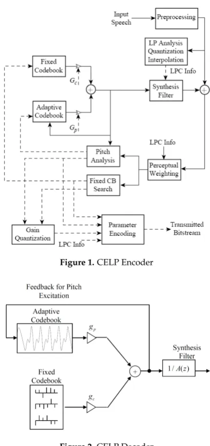
Block diagrams of a Code-Excited Linear Prediction (CELP) encoder and decoder are shown in 61
Figs.1and2, respectively [1,2]. 62
We provide a brief description of the various blocks in Figs.1and2to begin. The CELP encoder is an implementation of the Analysis-by-Synthesis (AbS) paradigm [1]. CELP, like most speech codecs in the last 45 years, is based on the linear prediction model for speech, wherein the speech is modeled as
s(k) =
N
∑
i=1ais(k−i) +Gw(k) (1)
where we see that the current speech sample at time instantkis represented as a weighted linear 63
combination ofNprior speech samples plus an excitation term at the current time instant. The weights, 64
ai,i=1, 2, ....,N, are called the linear prediction coefficients. The Synthesis Filter in Fig.1has the form 65
of this linear combination of past outputs and the Fixed and Adaptive Codebooks model the excitation, 66
w(k). The LP Analysis block calculates the linear prediction coefficients, and we see that the block also 67
quantizes the coefficients so that encoder and decoder use exactly the same coefficients. 68
The adaptive codebook is used to capture the long term memory due to the speaker pitch and 69
the fixed codebook is selected to be an algebraic codebook, which has mostly zero values and only a 70
relatively few nonzero pulses. The Pitch Analysis block calculates the Adaptive Codebook long term 71
memory. The process is AbS in that for a block of (say)Minput speech samples, the linear prediction 72
coefficients and long term memory are calculated and a perceptual weighting filter is constructed 73
using the linear prediction coefficients. Then, for every lengthMsequence (codevector) in the Fixed 74
Codebook, (say) there areLcode vectors in the Fixed Codebook, a synthesized sequence of speech 75
Figure 1.CELP Encoder
Figure 2.CELP Decoder
the Fixed Codebook in terms of the lengthMsynthesized sequence that best matches the input block 77
of lengthMbased on minimizing the perceptually weighted squared error is chosen, and transmitted 78
to the CELP Decoder along with the long term memory, the predictor coefficients and the codebook 79
gains. These operations are represented by the Parameter Encoding block in Fig.1[1,10]. 80
The CELP Decoder uses these parameters to synthesize the block ofM reconstructed speech 81
samples presented to the listener as shown in Fig.2. There is also Post-Processing not shown in the 82
figure. 83
The quality and intelligibility of the synthesized speech is often determined by listening tests that 84
produce Mean Opinion Scores (MOS), which for narrowband speech vary from 1 up to 5 [11,12]. A 85
well-known codec such as G.711 is usually included to provide an anchor score value with respect to 86
which other narrowband codecs can be evaluated [13–15]. 87
It would be helpful to be able to associate a separate contribution to the overall performance by 88
each of the main components in Fig. 2, namely the Fixed Codebook, the Adaptive Codebook, and 89
the Synthesis Filter. Signal to Quantization Noise Ratio (SNR) is often used for speech waveform 90
characteristic of CELP codecs that is well known is that those speech attributes not captured by the 92
short term predictor must be accounted for, as best as possible, by the excitation codebooks, but an 93
objectively meaningful measure of the individual component contributions is yet to be advanced. 94
In the next section, we propose a decomposition in terms of the mutual information and 95
conditional mutual information with respect to the input speech provided by each component in the 96
CELP structure that appears particularly useful and interesting for capturing the performance and the 97
tradeoffs involved. 98
3. A Mutual Information Decomposition 99
Gibson [5] proposed the following decomposition of the several contributions to the synthesized speech by the CELP codec components. In particular, lettingXrepresent a frame of input speech samples, we defineXR,XN, andXCas the reconstructed speech, the prediction component, and the combined fixed and adaptive codebook components, respectively. Then we can write the mutual information between the input speech and the reconstructed speech as
I(X;XR) =I(X;XN,XC) =I(X;XN) +I(X;XC|XN) (2) This expression states that the mutual information between the original speechXand the reconstructed speechXRequals the mutual information betweenXandXN, theNthorder linear prediction ofX, plus the mutual information betweenXand the combined codebook excitationsXCconditioned on XN. Thus, to achieve or maintain a specified mutual information between the original speech and the reconstructed speech, any change inXNmust be offset by an adjustment ofXC. This fits what is known experimentally and that was alluded to earlier. If we defineXAto represent the Adaptive codebook contribution andXFto represent the Fixed codebook contribution, we can further decompose I(X;XC|XN)as
I(X;XC|XN) =I(X;XA,XF|XN)
=I(X;XA|XN) +I(X;XF|XN,XA)
=I(X;XF|XN) +I(X;XA|XN,XF)
(3)
where we have used the chain rule for mutual information [16]. 100
While these expressions are interesting, the challenge that remains is to characterize each of these 101
mutual informations without actually having to calculate them directly from data, which is a difficult 102
problem in and of itself [17]. 103
An interesting quantity introduced and analyzed by Gibson in a series of papers is the log ratio 104
of entropy powers [5,8,9]. Specifically, the log ratio of entropy powers is related to the difference in 105
mutual information, and further, in many cases, the entropy powers can be replaced with the minimum 106
mean squared prediction error (MMSPE) in the ratio. Using the MMSPE, the difference in mutual 107
informations can be easily calculated. The following sections develop these concepts before we apply 108
them to an analysis of the CELP structure. 109
4. Entropy Power/Entropy Rate Power 110
Given a random variableXwith probability density functionp(x), we can write the differential entropy h(X) = −R∞
−∞p(x)logp(x)dx where the variance var(X) = σ2. Since the Gaussian
distribution has the maximum differential entropy of any distribution with mean zero and varianceσ2
[16],
h(X)≤ 1
2log 2πeσ
2 (4)
from which we obtain
Q= 1
(2πe)exp 2h(X)≤σ
whereQwas defined by Shannon to be theentropy powerassociated with the differential entropy of 111
the original random variable [7]. In addition to defining entropy power, this equation shows that 112
the entropy power is theminimum variancethat can be associated with the not-necessarily-Gaussian 113
differential entropyh(X). 114
5. Cascaded Signal Processing 115
Figure3shows a cascade ofNsignal processing operations with the Estimator blocks at the output of each stage as studied by Messerschmitt [18]. He used the conditional mean at each stage and the corresponding conditional mean squared errors to obtain a representation of the distortion contributed by each stage. We analyze the cascade connection in terms of information theoretic quantities, such as mutual information, differential entropy, and entropy rate power. Similar to Messerschmitt, we consider systems that have no hidden connections between stages other than those explicitly shown. Therefore, we conclude directly from the Data Processing Inequality [16] that
I(X;Y1)≥...≥I(X;YN−1)≥I(X;YN)≥ I(X;Xb) (6) SinceI(X;Yn) =h(X)−h(X|Yn), it follows from Eq. (6) that for non-negativeh(·),
h(X|Y1)≤...≤h(X|YN−1)≤h(X|YN)≤h(X) (7) For the optimal estimators at each stage, the basic Data Processing Inequality also yieldsI(X;Yn)≥ 116
I(X;Xbn)and thush(X|Yn)≤h(X|Xbn). These are the fundamental results that additional processing
Figure 3.N-Link System Block Diagram (Adapted from [18])
117
cannot increase the mutual information. 118
Now we notice that the series of inequalities in Eq. (7) along with the entropy power expression 119
in Eq. (5) gives us the series of inequalities in terms of entropy power at each stage in the cascaded 120
signal processing operations 121
QX|Y1 ≤...≤QX|YN−1 ≤QX|YN ≤QX (8) We can also write that
QX|Yn≤QX|Xbn (9)
In the context of Eq. (8), the notationQX|Yndenotes the minimum variance when reconstructing 122
6. Log Ratio of Entropy Powers 124
We can use the definition of the entropy power in Eq. (5) to express the logarithm of the ratio of two entropy powers in terms of their respective differential entropies as [8]
logQX QY
=2[h(X)−h(Y)] (10)
We can write a conditional version of Eq. (5) as
QX|Yn = 1
(2πe)exp 2h(X|Yn)≤Var(X|Yn) (11)
and from which we can express Eq. (10) in terms of the entropy powers at successive stages in the signal processing chain, Fig.3, as
1 2log
QX|Yn QX|Yn−1
=h(X|Yn)−h(X|Yn−1) (12)
If we add and subtracth(X)to the right hand side of Eq. (12), we then obtain an expression in terms of the difference in mutual information between the two stages as
1 2log
QX|Yn QX|Yn−1
= I(X;Yn−1)−I(X;Yn) (13)
From the series of inequalities on the entropy power in Eq. (8), we know that both expressions in Eqs. 125
(12) and (16) are greater than or equal to zero. 126
These results are from [8] and extend the Data Processing Inequality by providing a new 127
characterization of the information loss between stages in terms of the entropy powers of the two 128
stages. Since differential entropies are difficult to calculate, it would be particularly useful if we could 129
obtain expressions for the entropy power at two stages and then use Eqs. (12) and (16) to find the 130
difference in differential entropy and mutual information between these stages. 131
We are interested in studying the change in the differential entropy and mutual information 132
brought on by different signal processing operations by investigating the log ratio of entropy powers. 133
In the following we highlight several cases where Eq. (10) holds with equality when the entropy powers are replaced by the corresponding variances. The Gaussian and Laplacian distributions often appear in studies of speech processing and other signal processing applications[10,15,19], so we show that substituting the variances for entropy powers in the log ratio of entropy powers for these distributions satisfies Eq. (10) exactly. For two i.i.d. Gaussian distributions with zero mean and variancesσ2XandσY2, we have directly thatQX=σX2 andQY=σY2, so
1 2log
QX QY
= 1
2log
σX2
σY2
= [h(X)−h(Y)] (14)
which satisfies Eq. (10) exactly. Of course, since the Gaussian distribution is the basis for the definition 134
of entropy power, this result is not surprising. 135
For two i.i.d. Laplacian distributions with variancesλ2Xandλ2Y[20], their corresponding entropy
powersQX=2eλ2X/πandQY=2eλ2Y/π, respectively, so we form
1 2log
QX QY
=1
2log
λ2X
λ2Y
=[h(X)−h(Y)].
sinceh(X) =ln(2eλX)so the Laplacian distribution also satisfies Eq. (10) exactly [5]. We thus conclude 136
that we can substitute the variance, or for zero mean Laplacian distributions, the mean squared value 137
for the entropy power in Eq. (10) and the result is the difference in differential entropies. 138
Interestingly, using mean squared errors or variances in Eq. (10) is accurate for many other 139
distributions as well. It is straightforward to show that Eq. (10) holds with equality when the entropy 140
powers are replaced by mean squared error for the logistic, uniform, and triangular distributions 141
as well. Further, the entropy powers can be replaced by the ratio of the squared parameters for the 142
Cauchy distribution. 143
Therefore, the satisfaction of Eq. (10) with equality occurs in more than one or two special cases. 144
The key points are first that the entropy power is the smallest variance that can be associated with 145
a given differential entropy, so the entropy power is some fraction of the mean squared error for 146
a given differential entropy. Second Eq. (10) utilizes the ratio of two entropy powers, and thus, if 147
the distributions corresponding to the entropy powers in the ratio are the same, the scaling constant 148
(fraction) multiplying the two variances will cancel out. Therefore, we are not saying that the mean 149
squared errors equal the entropy powers in any case but for Gaussian distributions. It is the new 150
quantity, the log ratio of entropy powers that enables the use of the mean squared error to calculate the 151
loss in mutual information at each stage. 152
7. Mutual Information in the Short Term Prediction Component 153
Gibson [5] used Eq. (16) to investigate the change in mutual information as the predictor order, 154
denoted in the following byN, is increased for different speech frames. Based on several analyses 155
of the MMSPE and the fact that the log ratio of entropy powers can be replaced with the log ratio of 156
MMSPE’s for several different distributions, as outlined in Sec.6and in [9], we can use the expression 157
1 2log
MMSPE(X,XN−1) MMSPE(X,XN)
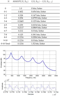
=I(X;XN)−I(X;XN−1) (16) as in [5] to associate a change in mutual information with a change in the predictor order. Figure 158
4(bottom) shows 160 time domain samples from a narrowband (200 to 3400 Hz) speech sentence 159
sampled at 8,000 samples/sec, and the top plot is the magnitude of the spectral envelope calculated 160
from the linear prediction model using Eq. (1). We show theMMSPEand the corresponding change in 161
mutual information for predictor ordersN=1, 2, ..., 10, in Table1. We see that the mutual information 162
between the input speech frame and a 10thorder predictor is 1.52 bits/sample. We can examine the 163
mutual information between the input speech and a 10thorder linear predictor for other frames in the 164
same speech utterance. 165
To categorize for easy reference the differences in the speech frames, we use a common indicator of predictor performance, the Signal-to-Prediction Error (SPER) in dB [21], also called the Prediction Gain [15], defined as
SPER(dB) =10 log10 MSE(X) MMSPE(X,X10)
(17)
whereMSE(X)is the average energy in the utterance andMMSPE(X,X10)is the minimum mean 166
squared prediction error achieved by a 10thorder predictor. TheSPERcan be calculated for any 167
predictor order but we choose N = 10, a common choice in narrowband speech codecs and the 168
predictor order that, on average, captures most of the possible reduction in mean squared prediction 169
error without including long term pitch prediction. For a normalizedMSE(X) =1.0, we see that for 170
the speech frame in Fig.4, theSPER=9.15 dB. 171
Several other speech frames by the same speaker are analyzed in [5] and the results for these 172
frames are tabulated in Table5. From this table, it is evident that the mutual information between 173
the input speech and a 10thorder linear predictor can change quite dramatically across frames, even 174
with the same speaker. We observe that the change in mutual information in some sense mirrors a 175
Table 1.Change in Mutual Information from Eq. (16) as the Predictor Order is Increased: Frame 3237, SPER=9.15dB
N MMSPE(X,XN) I(X;XN)−I(X;XN−1)
0 1.0 0 bits/letter
0-1 0.402 0.656 bits/letter
1-2 0.328 0.147 bits/letter
2-3 0.294 0.0795 bits/letter
3-4 0.2465 0.125 bits/letter
4-5 0.239 0.0234 bits/letter
5-6 0.2117 0.0869 bits/letter
6-7 0.212 0.0 bits/letter
7-8 0.125 0.381 bits/letter
8-9 0.1216 0.0206 bits/letter
9-10 0.1216 0.0 bits/letter
0-10 Total 0.1216 1.52 bits/letter
Figure 4.Frame 3237 Time Domain Waveform (Bottom) and Spectral Envelope, SPER = 9.15 dB
characterization in terms of mutual information is new and allows new analyses of the performance 177
of CELP codecs in terms of bits/sample reduction in rate that can be associated with the short term 178
predictor. We provide this analysis in Sec.9. 179
8. Mutual Information in the Fixed and Adaptive Codebooks 180
How do we find the change in mutual information provided by the Adaptive Codebook and 181
the Fixed Codebook? The Adaptive Codebook relies on long term prediction to model the vocal 182
tract excitation due to the speaker pitch. As such, an approach similar to that used for the short 183
term or linear predictor is possible. The Fixed Codebook contribution in terms of bits/sample is less 184
direct. We could attempt to estimate the codebook complexity or we could simply use the number 185
of bits/sample used to transmit the Fixed Codebook excitation. We elaborate on each of these in the 186
Table 2.Change in Mutual Information from Eq. (16) for 10thOrder Predictors and Corresponding SPERs for Several Speech Frames [5]
Speech Frame No. SPERin dB I(X;X10)−I(X;X0)
45 16 2.647 bits/letter
23 11.85 1.968 bits/letter
3314 7.74 1.29 bits/letter
87 5 0.83 bits/letter
8.1. Adaptive Codebook: Long Term Prediction 188
The long term predictor that makes up the adaptive codebook in CELP may have 1 or 3 taps and is of the form
P(z) =β−1z−(P−1)+β0z−P+β1z−(P+1) (18) whereβi,i= −1, 0, 1, are the predictor coefficients that are updated on a frame by frame basis and Pis the lag of the periodic correlation that captures the pitch excitation of the vocal tract. A 3 tap predictor as shown in Eq. (18) requires a stability check to guarantee that this component does not cause divergence [22]. The single tap form given by
P(z) =βz−P (19)
only needs the stability check that|β|<1, which should hold for any normalized autocorrelation. The
189
3 tap form can often provide improved performance over the single tap predictor, but at increased 190
complexity. 191
We denote the long term predicted value asXPPto distinguish it from the short term predictor of 192
orderN,XN, which contains all terms up to and includingN. Thus, we can write the MMSPE between 193
XandXP
PasMMSPE(X,XPP). 194
The prediction gain in dB is often used as a performance indicator for a pitch predictor. The long 195
term prediction gain has the form of Eq. (17) but withMMSPE(X,X10)replaced byMMSPE(X,XPP), 196
whereXPPis the long term predicted value for a pitch lag ofPsamples, where usuallyP=20 up to 197
P=140 samples at 8000 samples/sec. Rather than calculate the prediction gain for selected speech 198
frames, we consult the literature to get a range of values that might be expected. 199
Cuperman and Pettigrew [23] indicate a pitch prediction gain of 1 to 5 dB, but with around 2 dB 200
on the average. Other sources indicate that the prediction gains can be 3-4 dB [24] or up to 5-6 dB [25]. 201
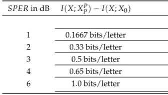
Table3shows the mutual information in bits/letter that can be associated with prediction gains of 1, 2, 202
3, 4, and 6 dB. 203
It is interesting to consult the standardized speech codecs to see how many bits/sample are 204
allocated to coding the pitch gain (coefficient or coefficients) and the pitch delay (lag). For the 205
narrowband form of the AMR codec, we see that for 7.95 bits/sec rate, the pitch gain and pitch delay 206
are allocated 16 and 28 bits, respectively, per 20 msec frame, or 44 bits/160 samples = 0.275 bits/sample 207
[3]. For the highest rate of 12.2 kbits/sec, pitch gain and delay are allocated 46 bits/160 samples = 208
0.2875 bits/sample. Consulting Table3, we see that this corresponds to anSPERof between 1 and 2 209
dB. 210
8.2. Fixed Codebook 211
The most often used fixed codebooks in popular speech coders, are sparse and have several 212
shifted phase tracks, where each track consists of equally spaced pulses with 4 or 5 zero values in 213
Table 3.Change in Mutual Information from Eq. (16) for Various Pitch Predictors and Corresponding SPER
SPERin dB I(X;XP
P)−I(X;X0)
1 0.1667 bits/letter 2 0.33 bits/letter 3 0.5 bits/letter 4 0.65 bits/letter 6 1.0 bits/letter
tracks in some specific order. Getting an estimate of the number of bits/sample to be associated with a 215
fixed codebook is therefore challenging. However, we know a few specific things. 216
The initial studies of analysis-by-synthesis codecs used Gaussian random sequences as the 217
excitation. In particular, Atal and Schroeder used 1024 Gaussian random sequences that were 40 218
samples long. Thus, this codebook used 10 bits/40 samples or 0.25 bits/sample [26]. However, this 219
does not include the fixed codebook gain. The U. S. Federal Standard FS1016 CELP at 4.8 kbits/sec has 220
allocations of 56 bits per frame of 240 samples or 0.233 bits/sample to the fixed codebook [10]. For a 221
CELP codec that operates at 6 kbits/sec and above and a sparse codebook with five tracks and 8 pulses 222
per track, an estimate of 3 bits plus a sign bit per track gives a fixed codebook rate of 0.5 bits/sample 223
[24]. 224
The narrowband AMR codec at 7.95 kbits/sec allocates 88 bits/20 msec frame or 0.55 bits/sample 225
to the fixed codebook, and at 12.2 kbits/sec, 1 bit/sample is devoted to the fixed codebook gain and 226
delay [3]. Thus, we see that at around 4 kbits/sec the allocation is about 0.25 bits/sample, at 8 kbits/sec 227
the fixed codebook gets about 0.5 bits/sample, and at 12.2 kbits/sec, 1 bit/sample. 228
We now have estimates of the bits/sample devoted to the short term predictor, adaptive codebook, 229
and fixed codebook for a CELP codec operating at different bit rates. We show how to exploit these 230
estimates in the following to predict the rate of CELP codecs for different speech sources. 231
9. Estimated versus Actual CELP Codec Performance 232
The analyses determining the mutual information in bits/sample between the input speech and 233
the short term linear prediction, the adaptive codebook, and the fixed codebook individually, are 234
entirely new and provide new ways to analyze CELP codec performance by only analyzing the input 235
source. In this section we estimate the performance of a CELP codec by analyzing the input speech 236
source to find the mutual information provided by each CELP component about the input speech, and 237
then subtracting the three mutual informations from a reference codec rate in bits/sample for a chosen 238
MOS value to get the final estimate of the rate required in bits/sample to achieve the target MOS. 239
For waveform speech coding, such as differential pulse code modulation (DPCM), for a particular 240
utterance, we can study the rate in bits/sample versus the mean squared reconstruction error or SNR 241
to obtain some idea of the codec performance for this input speech segment [14,15]. However, while 242
SNR may order DPCM subjective codec performance correctly, it does not provide an indicator of the 243
actual difference in subjective performance. Subjective performance is most accurately available by 244
conducting subjective listening tests to obtain Mean Opinion Scores (MOS); alternatively, reasonable 245
views of subjective performance can be obtained from software such as PESQ/MOS [12]. We use the 246
latter. In either case, however, MOS cannot be generated on a per frame basis as listening tests and 247
PESQ values are generated from longer utterances. 248
Therefore, we cannot use the per frame estimates of mutual information from Sec.7and need to 249
calculate estimates of mutual information over longer sentences. Toward this end, Table4contains 250
autocorrelations for two narrowband (200 to 3400 Hz) utterances sampled at 8,000 samples/sec, "We 251
Table 4.Composite Source Models for Narrowband Speech Sentences[6]
Sequence Mode Autocorrelation coefficients for V, ON, H Mean Square Probability Average frame energy for UV Prediction Error
“lathe" V [1 0.8217 0.5592 0.3435 0.1498 0.0200 0.0656 0.5265
(Female) −0.0517−0.0732−0.0912−0.1471−0.2340]
(active speech level:−18.1 dBov) ON [1 0.8495 0.5962 0.3979 0.2518] 0.0432 0.0093
(sampling rate: 8 kHz) H [1 0.2709 0.2808 0.1576 0.1182] 0.7714 0.0186
UV 0.1439 0.1439 0.0771
S 0.3685
“we were away" V [1 0.8014 0.5176 0.2647 0.0432−0.1313 0.0780 0.9842
(Male) −0.2203−0.3193−0.3934−0.4026−0.3628]
(active speech level:−16.5 dBov) ON [1 0.8591 0.7215 0.6128 0.5183] 0.0680 0.0053
(sampling rate: 8 kHz) H 0
UV 0
S 0.0105
Table 5.Rate in Bits[5]
Speech Frame No. SPERin dB I(X;X10)−I(X;X0)
45 16 2.647 bits/letter 23 11.85 1.968 bits/letter 3314 7.74 1.29 bits/letter
87 5 0.83 bits/letter
by a female, including the decomposition of the sentences into five modes, namely, Voiced, Unvoiced, 253
Onset, Hangover, and Silence, and their corresponding relative frequencies. These data are excerpted 254
from tables in Gibson and Hu [6], and are not calculated on a perframe basis but averaged over all 255
samples of the utterance falling in the specified subsource model. 256
From Table4, the Voiced subsource models are set asN=10thorder, with the 1 in the column 257
vector representing thea0th=1 term. The Onset and Hangover modes are modeled asN=4thorder 258
autoregressive (AR). We see from this table that the sentence "We were away . . . ," is Voiced with a 259
relative frequency of 0.98, and that the sentence "A lathe is a big . . . ," has a breakdown of Voiced 260
(0.5265), Silence (0.3685), Unvoiced (0.0771), Onset (0.0093), and Hangover (0.0186). TheMMSPEsfor 261
each mode are also shown in the table. 262
We focus on G.726 as our reference codec. Generally, G.726 ADPCM at 32 kbits/sec or 4 263
bits/sample for narrowband speech is considered to be "toll quality." G.726 is selected as the reference 264
codec because ADPCM is a waveform-following codec and is the best performing speech codec which 265
does not rely on a more sophisticated speech model. In particular, G.726 utilizes only two poles 266
and six zeros and the parameter adaptation algorithms rely only on polarities. G.726 will track pure 267
tones as well as other temporal waveforms in addition to speech. In G.726, no parameters are coded 268
and transmitted, only the quantized and coded prediction error signal. Finally, both mean squared 269
reconstruction error or SNR and MOS have meaning for G.726, which is useful since SPER plays a role 270
in estimating the change in mutual information from the log ratio of entropy powers. 271
From Tables6and7, G.726 achieves a PESQ/MOS of about 4.0 for 4 bits/sample and for both 272
sentences, "We were away a year ago," spoken by a Male Speaker and "A lathe is a big tool. Grab every 273
dish of sugar," spoken by a Female [6]. Therefore, we use 4 bits/sample as our reference point for toll 274
quality speech for these two sentences. We then subtract from the rate of 4 bits/sample, the rates in 275
bits/sample we associate with each of the CELP codec components as estimated from Secs.7and8. 276
For "We were away . . . ," we see from Table4that the 10thorder model of the Voiced mode has a 277
MMSPE=0.078, which corresponds to a mutual information reduction of 1.84 bits/sample. For this 278
highly voiced sentence, we estimate the mutual information corresponding to the adaptive codebook 279
as 0.5 bits/sample, and at a codec rate of 8,000 bits/sec, the fixed codebook mutual information would 280
correspond to 0.5 bits/sample. Silence corresponds to about only 1 percent of the total utterance. If we 281
Table 6.Codec Rates to Achieve PESQ-MOS of 4.0 for We were away[6]
Codec Rbits/sample
G.726 4.0 bits/sample G.729 1.1 bits/sample AMR 1.1 bit/sample
Table 7.Codec Rates to Achieve PESQ-MOS of 4.0 for Lathe[6]
Codec Rbits/sample
G.726 4.0 bits/sample G.726 w/CNG 2.8 bits/sample G.729 1.0 bits/sample AMR 1.0 bit/sample
Inspecting Table6, the rates for the AMR and G.729 codecs at this MOS are 1.1 bits/sample, so there is 283
surprisingly good agreement. 284
From Table4, we see that for the utterance, "A lathe is . . . ," there is broader mix of speech 285
modes, including significant Silence and Unvoiced components. Neither of these modes had to be 286
dealt with for the sentence "We were away . . . ." Since Silence is almost never perfect silence and 287
usually consists of low level background noise, we associate the bits/sample for Silence with a silence 288
detection/comfort noise generation (CNG) method [24]. From Table7, we see that G.726 w/CNG is 289
about 1.2 bits/sample lower than G.726, even though it occurs for only 0.3685 portion of the utterance. 290
For the short term prediction, theMMSPE= 0.0656 which corresponds to a mutual information of 291
1.96 bits/sample. The adaptive codebook contribution at 8 kbits/sec, can again be estimated as 0.5 292
bits/sample, and the fixed codebook component estimated at 0.5 bits/sample. 293
If we now combine all of these estimates with their associated relative frequencies of occurrence as 294
indicated in Table4, we obtain a total mutual information of 0.5265(1.96 + 0.5) + 1.2 + 0.5(0.0771) = 2.5 295
bits/sample. Subtracting this from 4 bits/sample, we estimate that the CELP codec rate in bits/sample 296
for an MOS = 4.0 would be 1.5 bits/sample. We see from Table7that for AMR and G.729 their rate is 297
1.0 bits/sample. This gap can be narrowed if the adaptive codebook contribution is toward the upper 298
end of the expectedSPERof say 6 dB. In this case the Voiced component has the mutual information of 299
0.5265(1.96 + 1.0) = 1.56 so the total mutual information is 2.8, and then subtracting from 4 bits/sample 300
we obtain a CELP codec rate estimate of 1.2 bits/sample to achieve an MOS = 4.0. The actual CELP rate 301
needed by G.729 and AMR for this MOS is about 1.0 bits/sample, which constitutes good agreement. 302
10. Conclusions 303
We have introduced a new approach to estimating CELP codec performance on a particular 304
speech utterance by analysis of the input speech source only. That is, a particular CELP codec does not 305
need to be implemented and used to process the speech. We have presented examples that illustrate the 306
steps in the process and the accuracy of the estimated performance. While the power of the approach 307
is evident, it is clear that many more sentences need to be processed to gain experience in estimating 308
the various components. However, this approach offers the possibility of conducting performance 309
analyses prior to the implementation of new CELP codec architectures and perhaps other new speech 310
codec designs. It is striking that estimates of codec performance are possible while only knowing the 311
source model and the distortion measure. Thus, in one sense, this new method parallels rate distortion 312
theory. 313
Funding:This research received no external funding.
314
Conflicts of Interest:The authors declare no conflict of interest.
316 Abbreviations
Thefollowingabbreviationsareusedinthismanuscript:
317 318
AR Autoregressive
ADPCM Adaptive differential pulse code modulation
AMR Adaptive multirate
AbS Analysis-by-Synthesis
CELP Code-excited linear prediction
CNG Comfort noise generation
DPCM Differential pulse code modulation
EVS Enhanced voice services
MOS Mean Opinion Score
MSPE Mean squared prediction error
MMSPE Minimum mean squared prediction error
MMSE Minimum mean squared error
SNR Signal to quantization noise ratio
SPER Signal to prediction error ratio
VoIP Voice over Internet Protocol
319
320
1. Chen, J.H.; Thyssen, J. Analysis-by-Synthesis Speech Coding. InSpringer Handbook of Speech Processing;
321
Springer, 2008.
322
2. Gibson, J. Speech Compression. Information2016,32.
323
3. ETSI. 3GPP AMR Speech Codec; Transcoding Functions. Technical report, ETSI, 2002.
324
4. Dietz, M.; Multrus, M.; Eksler, V.; Malenovsky, V.; Norvell, E.; Pobloth, H.; Miao, L.; Wang, Z.; Laaksonen,
325
L.; Vasilache, A.; Kamamoto, Y.; Kikuiri, K.; Ragot, S.; Faure, J.; Ehara, H.; Rajendran, V.; Atti, V.; Sung, H.;
326
Oh, E.; Yuan, H.; Zhu, C. Overview of the EVS codec architecture. Proc. Speech and Signal Processing
327
(ICASSP) 2015 IEEE Int. Conf. Acoustics, 2015, pp. 5698–5702. doi:10.1109/ICASSP.2015.7179063.
328
5. Gibson, J.D. Entropy Power, Autoregressive Models, and Mutual Information.Entropy2018.
329
6. Gibson, J.D.; Hu, J. Rate distortion bounds for voice and video. Foundations and TrendsR in Communications
330
and Information Theory2014,10, 379–514.
331
7. Shannon, C.E. A mathematical theory of communication. Bell Sys. Tech. Journal1948,27, 379–423.
332
8. Gibson, J.D. Log Ratio of Entropy Powers. UCSD Information Theory and Application Workshop, 2018.
333
9. Gibson, J.; Oh, H. Analysis of Cascaded Signal Processing Operations Using Entropy Rate Power. Asilomar
334
Conference on Signals,Systems and Computers, 2018.
335
10. Chu, W.C.Speech Coding Algorithms; Wiley, 2003.
336
11. Grancharov, V.; Kleijn, W.B. Speech Quality Assessment. InSpringer Handbook of Speech Proceessing; Springer,
337
2008.
338
12. ITU-T Recommendation P.862. Perceptual Evaluation of Speech Quality (PESQ), an objective method for
339
end-to-end Speech Quality Assessment of Narrow-band telephone networks and Speech Codecs. 2001.
340
13. Kleijn, W.B. Principles of Speech Coding. InSpringer Handbook of Speech Proceessing; Springer, 2008.
341
14. Gibson, J.D.; Berger, T.; Lookabaugh, T.; Lindbergh, D.; Baker, R.L. Digital Compression for Multimedia:
342
Principles and Standards; Morgan Kaufmann Publishers Inc.: San Francisco, CA, 1998.
343
15. Rabiner, L.R.; Schafer, R.W.Digital processing of speech signals; Pearson, 2011.
344
16. Cover, T.M.; Thomas, J.A.Elements of Information Theory; Wiley-Interscience, 2006.
345
17. Darbellay, G.A.; Vajda, I. Estimation of the information by an adaptive partitioning of the observation
346
space. IEEE Transactions on Information Theory1999,45, 1315–1321. doi:10.1109/18.761290.
347
18. Messerschmitt, D.G. Accumulation of Distortion in tandem Communication links. IEEE Trans. on
348
Information Theory1979,IT-25, 692–698.
349
19. Gray, R.M.Linear Predictive Coding and the Internet Protocol; NOW: Hanover, MA, USA, 2010.
350
20. Shynk, J.J.Probability, random variables, and random processes: theory and signal processing applications; John
351
Wiley & Sons: Hoboken,NJ, USA, 2012.
352
21. Sayood, K.Introduction to data compression; Morgan Kaufmann: Waltham, MA, USA, 2017.
22. Ramachandran, R.P.; Kabal, P. Pitch prediction filters in speech coding. and Signal Processing IEEE
354
Transactions on Acoustics, Speech1989,37, 467–478. doi:10.1109/29.17527.
355
23. Cuperman, V.; Pettigrew, R. Robust low-complexity backward adaptive pitch predictor for
356
low-delay speech coding. Speech and Vision IEE Proceedings I-Communications 1991, 138, 338–344.
357
doi:10.1049/ip-i-2.1991.0044.
358
24. Kondoz, A.M.Digital Speech: Coding for Low Bit Rate Communication Systems; Wiley, 2004.
359
25. Kleijn, W.B.; Paliwal, K.K.Speech Coding and Synthesis; Elsevier, 1995.
360
26. Schroeder, M.; Atal, B. Code-excited linear prediction(CELP): High-quality speech at very low bit rates.
361
Proc. and Signal Processing ICASSP ’85. IEEE Int. Conf. Acoustics, Speech, 1985, Vol. 10, pp. 937–940.
362
doi:10.1109/ICASSP.1985.1168147.
![Figure 3. N-Link System Block Diagram (Adapted from [18])](https://thumb-us.123doks.com/thumbv2/123dok_us/994490.1599162/5.595.152.433.396.511/figure-n-link-block-diagram-adapted.webp)
![Table 2. Change in Mutual Information from Eq. (16) for 10th Order Predictors and CorrespondingSPERs for Several Speech Frames [5]](https://thumb-us.123doks.com/thumbv2/123dok_us/994490.1599162/9.595.165.430.124.210/table-change-mutual-information-predictors-correspondingspers-speech-frames.webp)
![Table 4. Composite Source Models for Narrowband Speech Sentences[6]](https://thumb-us.123doks.com/thumbv2/123dok_us/994490.1599162/11.595.97.502.111.221/table-composite-source-models-narrowband-speech-sentences.webp)
![Table 6. Codec Rates to Achieve PESQ-MOS of 4.0 for We were away[6]](https://thumb-us.123doks.com/thumbv2/123dok_us/994490.1599162/12.595.218.380.202.274/table-codec-rates-achieve-pesq-mos-away.webp)
