An improved projection of climate observations for detection and attribution

https://doi.org/10.5194/ascmo-5-161-2019 © Author(s) 2019. This work is distributed under the Creative Commons Attribution 3.0 License.

An improved projection of climate observations for

detection and attribution

Alexis Hannart1,2 1_{Ouranos, Montreal, Canada}

2_{IFAECI, CNRS-CONICET-UBA, Buenos Aires, Argentina}

Correspondence:Alexis Hannart ([email protected])

Received: 14 March 2016 – Revised: 23 April 2018 – Accepted: 26 May 2018 – Published: 26 November 2019

Abstract. An important goal of climate research is to determine the causal contribution of human activity to observed changes in the climate system. Methodologically speaking, most climatic causal studies to date have been formulating attribution as a linear regression inference problem. Under this formulation, the inference is often obtained by using the generalized least squares (GLS) estimator after projecting the data on ther leading eigenvectors of the covariance associated with internal variability, which are evaluated from numerical climate models. In this paper, we revisit the problem of obtaining a GLS estimator adapted to this particular situation, in which only the leading eigenvectors of the noise’s covariance are assumed to be known. After noting that the eigenvectors associated with the lowest eigenvalues are in general more valuable for inference purposes, we introduce an alternative estimator. Our proposed estimator is shown to outperform the conventional estimator, when using a simulation test bed that represents the 20th century temperature evolution.

1 Introduction

1.1 Context

An important goal of climate research is to determine the causes of past global warming in general and the responsibil-ity of human activresponsibil-ity in particular (Hegerl et al., 2007); this question has thus emerged as a research topic known as de-tection and attribution (D&A). From a methodological stand-point, D&A studies are usually based on linear regression methods, often referred to in this particular context as opti-mal fingerprinting, whereby an observed climate change is regarded as a linear combination of several externally forced signals added to internal climate variability (Hasselmann, 1979; Bell, 1986; North et al., 1982; Allen and Tett, 1999; Hegerl and Zwiers, 2011). On the one hand, the latter sig-nals consist of spatial, temporal or space–time patterns of response to external forcings as anticipated by one or sev-eral climate models. Internal climate variability, on the other hand, is usually represented by a centred multivariate Gaus-sian noise. Its covariance 6, which is also estimated from model simulations, thus describes the detailed space–time features of internal variability. In particular, its eigenvectors

can often be interpreted as the modes of variability, whose relative magnitudes are reflected by the associated eigenval-ues.

Denotingythen-dimensional vector of observed climate change,x=(x1, . . ., xp) then×pmatrix concatenating thep

externally forced signals andνthe internal climate variability noise, the regression equation is as follows:

y=xβ+ν. (1)

The results of the inference on the vector of regression co-efficients β, and the magnitude of its confidence intervals, determine whether the external signals “are present in the ob-servations” (Hegerl and Zwiers, 2011) and whether or not the observed change is attributable to each forcing.

Under the assumption that6 is known, the above infer-ence problem can be solved using the standard generalized least squares (GLS) setting (e.g. Amemiya, 1985). Under this framework, the expression of the best linear unbiased estima-tor (BLUE) and its variance are given by the following:

b

β=(x0₆−1_x)−1_(x0₆−1_{y), Var(} b

β)=(x0₆−1_x)−1_{. (2)}

trans-formed regression equation:

Ty=Txβ+Tν, (3)

where then×ntransformation matrixTis such that the com-ponents of the transformed noise Tν are independent and identically distributed (IID). This condition yieldsT6T0=I and an admissible choice forTis thus as follows:

T=V1−12_V0_{, (4)}

where 1=diag(λ1, . . ., λn) with λ1≥. . .≥λn>0 is the

matrix of eigenvalues of 6 andV=(v1, . . .,v_n) is its ma-trix of column eigenvectors, i.e.6=V1V0_{. In Eq. (3), the}

data are thus projected on the eigenvectors of the covariance matrix scaled by the inverse square root of their eigenvalues. In most applications, the covariance 6is not known and Eq. (2) cannot be implemented. This has given rise to many theoretical developments (e.g. Poloni and Sbrana, 2014; Naderahmadian et al., 2015) which often rely on further as-sumptions regarding the covariance6, in order to allow for its estimation simultaneously withβ. In the applicative con-text of D&A considered here, the situation may be viewed as an in-between between known and unknown6 because we have access to an ensemble of unforced climate model simulations. This ensemble can be used to extract valuable information about 6. However, the resulting knowledge of 6 is imperfect for two reasons. First, the size of the ensem-ble is often very small, typically a few dozens, because of the high cost of numerical experiments requiring intensive computational resources. For the range of dimensionsn usu-ally considered, typicusu-ally a few hundreds or thousands, the empirical covarianceSmay thus be non-invertible. Second, climate model simulations are known to inadequately rep-resent the modes of internal variability at the smaller scale. Those smaller scale modes have lower magnitude and are expected to be associated with eigenvectors with low values. Furthermore, the latter eigenvectors with low eigen-values are also poorly sampled by construction and therefore are difficult to estimate reliably (North et al., 1982). For these two reasons, it is often assumed that only a small numberr of leading eigenvectors of6, which are denoted (v1, . . .,vr)

andris typically on the order of 10, can be estimated from the control runs with enough reliability. Accordingly, it is as-sumed that the remainingn−reigenvectors and eigenvalues are unknown.

Under this assumption, the inference on β must there-fore be obtained based on theserleading eigenvectors only. The conventional approach presently used in D&A studies to tackle this problem follows from a simple and straightfor-ward idea: adapting Eq. (4) to this situation by restricting the image of the transformation matrixTto the subspace gener-ated by therleading eigenvectors, thus leading to a truncated transformation having the following expression:

Tr =Vr1 −1₂

r V0r, (5)

where 1r=diag(λ1, . . ., λr) and Vr=(v1, . . .,vr). A new

estimator thus follows by similarly applying the OLS esti-mator to the transformed data (Trx,Try):

b

βr=(x06−r1x)

−1_(x0₆−1

r y), (6)

where6−1

r =Vr1−r1Vr0 is the pseudo-inverse of Vr1rV0r.

Finally, from a mere terminology standpoint, applying the truncated transformationTr to the data is often referred to

in D&A as “projecting” the data onto the subspace spanned by the leading eigenvectors. However,Tris in fact not a

pro-jection from a mathematical standpoint insofar asT2_r 6=Tr

hence we prefer to use the word “transformation”.

1.2 Objectives

The solution recalled above in Eq. (6) is easy to use and may seem to be a natural choice. It emerged as a popular approach in D&A arguably for these reasons. Nevertheless, this ap-proach has two important limitations. Firstly, as pointed out by Hegerl et al. (1996), the leading eigenvectors sometimes fail to capture the signalsx. Indeed, the leading eigenvectors capture variability well, but not necessarily the signal, merely because the corresponding physical processes may differ and be associated with different patterns. Secondly, by construc-tion, the subspace spanned by the leading eigenvectors max-imizes the amplitude of the noise, thereby minimizing the ratio of signal to noise and affecting the performance of the inference onβ.

The first objective of this article is to highlight in detail these two limitations: both will be formalized and discussed immediately below in Sect. 2. Its second objective is to cir-cumvent these limitations by building a new estimator ofβ that performs better than the conventional estimator βbr of

Eq. (6) while still making the same assumptions and using the same data. Most importantly, the central assumption here is that only therleading eigenvectors of6can be estimated with enough accuracy from the control runs. Furthermore, we assume thatris given and is small compared ton(e.g.r is on the order of 10), and thatN control runs are available to estimate therleading eigenvectors withN≥r.

Section 2 highlights the limitations of the conventional es-timatorβbr. Section 3 introduces our proposed estimatorβb_r∗. Section 4 evaluates the benefit of our approach based on a realistic test bed, and illustrates it on actual observations of surface temperature. Section 5 concludes the paper.

2 Limitations of the conventional estimator

2.1 General considerations

of β. For this purpose, we propose to compare the variance Var(βb)=(x06

−1_x)−1_{of the BLUE estimator of Eq. (2)}

ob-tained by using the transformation matrixT=V1−12_V0_{, to} the variance of the estimatorβb−kobtained by using the

trans-formation matrixT−k=V−k1 −1₂ −kV

0

−k whereV−k and1−k

exclude the kth eigenvector and the kth eigenvalue respec-tively. From Eq. (2), these variances can be rewritten after some algebra:

Var(βb)=( n X i=1

x0v_iv0_ix/λi)−1Var(βb−k)

=( X

i=1,...,n i6=k

x0viv0ix/λi)−1. (7)

The Sherman–Morrison–Woodbury formula is a well known formula in linear algebra, which shows that the in-verse of a rank-one correction of some matrix, can be con-veniently computed by doing a rank one correction to the inverse of the original matrix. By applying the Sherman– Morrison–Woodbury formula to Eq. (7), we obtain the fol-lowing:

Var(βb−k)=Var(β)b+

Var(bβ−k)x0vkv0_kxVar(βb−k)

λk+v0_kxVar(βb−k)x0vk

. (8)

Unsurprisingly, an immediate implication of Eq. (8) is that removing any eigenvector vk results in an increase of the

variance of the estimator. Indeed, the matrix in the second term of the right-hand side of Eq. (8) is positive definite; it can thus be interpreted as the cost in variance increase of ex-cludingvk or conversely as the benefit in variance reduction

of including vk. Moreover, the most valuable eigenvectors

for inferringβin the above-defined sense are those combin-ing a small eigenvalue (low λk) and a good alignment with

the signals x (highx0vk). Accordingly, for any eigenvector

vk, its benefit is a decreasing function ofλk, everything else

being constant.

A similar conclusion can be reached by using a different approach. Consider this time the transformationT∗=x06−1. SinceT∗is ap×nmatrix, the data dimension is thus drasti-cally reduced fromntopin the transformed Eq. (3). Further-more, noting that the noise componentsT∗νhave covariance T∗_6T∗0_{, and applying the GLS estimator to the transformed}

data (T∗_y,T∗_{x), we obtain an estimator} b

β∗ which has the following expression:

b

β∗=(x0T∗(T∗6T∗0)−1T∗0x)−1(x0T∗(T∗6T∗0)−1T∗0y). (9)

After some algebra, the above expression ofbβ∗simplifies to the following:

b

β∗ =(x0₆−1_x)−1_(x0₆−1_{y), (10)}

which is exactly the expression of the estimator of Eq. (2). Therefore, remarkably, the BLUE estimator obtained from

the full data (y,x) is entirely recovered from the transformed data (T∗_y,T∗_{x) when using the subspace spanned by T}∗_.

The latter subspace can thus be considered as optimal, in the sense that it reduces the data dimension to its bare minimum pwhile still preserving all the available information for in-ferringβ. Thepdirections of the subspace spanned byT∗are denoted (u∗₁, . . ., u∗_p). They have the following expression:

u∗_k=

n X i=1

v0_ixk

λi

vi. (11)

Consistently with Eq. (8), Eq. (11) shows that for each k=1, . . ., p, the optimal directionu∗_k emphasizes the eigen-vectors that best trade off the smallest possible eigenvalue (i.e. small noise) with the best possible alignment between the eigenvector and the signal xk (i.e. strong signal). It is

interesting to notice that the foremost importance of small eigenvalues, which is underlined here, is also quite obvious in the formulation of optimal detection proposed by North and Stevens (1998). However, the importance of small eigen-values was lost later on, as truncation on leading eigenvectors became a popular practice.

In light of these considerations, the two main limita-tions of the conventional estimatorbβr of Eq. (6), mentioned

in Sect. 1, appear more clearly. Firstly, in agreement with Hegerl et al. (1996), there is no guarantee that the leading eigenvectors will align well with the signals at stake. Sec-ondly, the leading eigenvectors are by definition those with the largest eigenvalues. Therefore, a straightforward trunca-tion onto the leading eigenvectors, such as the one used inβbr,

maximizes the noise instead of minimizing it. While the first limitation may be an important pitfall in some cases, it will not be an issue whenever the signals align well with the lead-ing eigenvectors, which nothlead-ing prevents in general. In con-trast, the second limitation always manifests wheneverβbr is

used and is thus arguably a more serious problem of the con-ventional approach. In the present paper, we thus choose to focus restrictively on this second limitation, and to not ad-dress the first one.

2.2 Illustration

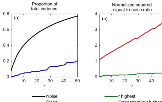
In order to illustrate the second issue more concretely, we use surface temperature data from Ribes and Terray (2012), de-scribed in more detail in Section 4. The signalsxconsidered here consist of the responses to anthropogenic and natural forcings, withp=2 andn=275. Bothxand the covariance 6are obtained from climate model simulations. Ther lead-ing eigenvectorsVr=(v1, . . .,vr) are obtained from6 and

are assumed to be known. The proportion of the noise’s to-tal variance retained by projecting the data onVr is denoted

r

10 20 30 40 50 0

0.2 0.4 0.6 0.8

Proportion of total variance

Noise Signal

r

10 20 30 40 50 0

1 2 3 4

Normalized squared signal-to-noise ratio

r highest

Orthogonal to r highest (b)

(a)

Figure 1.(a)Proportion of the total variance of the projected anthropogenic signalV0_rx1(thick blue line) and of the projected noiseV0rν (thick black line) as functions ofr; uniform increaser/n(light black line).(b)Signal-to-noise ratio of the projected data when using the projection subspaceVr consisting of therleading eigenvectors (thick green line) and when using the orthogonal subspaceV⊥r (thick red line) as functions ofr. Both values are normalized to the signal-to-noise ratio of the full data.

Vr is equal toVrVr0, we have the following:

σ_n2(r)=_E Var(Vc rV0rν)

/E Var(ν)c

=_E(ν0VrV0rν)/E(ν 0_ν)=

r X i=1

λi/ n X i=1

λi, (12)

σ_s2(r)=_E Var(Vc rV0rxi)

/E Var(xc i)

=x0_iVrV0rxi/xi0xi for i=1, . . ., p, (13)

where for any vectorz,Var(z) denotes the empirical variancec ofz. Figure 1a plotsσ_n2(r) andσ_s2(r) computed from Eq. (12) applied to the above-mentioned data. For simplicity, σ_s2(r) is shown only for the anthropogenic signalx1. As expected from the expression ofσ_n2(r) given in Eq. (12), it can be seen from this plot thatσ_n2(r) increases withr much faster than r/n, since by definition the leading eigenvectors concentrate most of the noise’s variance. In contrast,σ_s2(r) increases with rroughly liker/n: this shows that, in this example, the signal projects nearly uniformly on each eigenvector. For instance, whenr=20,Vr involves 7 % of theneigenvectors, and

ac-cordingly, projecting on Vr retains 8 % of the signal’s total

variance. In contrast, as much as 55 % of the noise’s total variance is retained by projecting onVr. Consequently, the

signal-to-noise ratio of the projected data (see Fig. 1b) is re-duced by a factor of 7 compared to the signal-to-noise ratio of the full data. Hence, it is fair to say that, in this case, the projection on the leading eigenvectors is greatly suboptimal, insofar as it drastically reduces the signal-to-noise ratio.

Let us now consider the quantitiesσ_n2∗(r) andσ_n2∗(r) de-fined as above, but projecting this time on the subspace

or-thogonal toVr. By construction,

σ_n2∗(r)=1−σ_n2(r),

σ_s2∗(r)=1−σ_s2(r). (14)

As a direct consequence, for r=20, the projection on the subspace orthogonal toVr captures 92 %=100 %–8 %

of the total variance of the signal, while the variance of the projected noise is only 20 %=100 %–80 % of the total. Therefore, the signal-to-noise ratio of the projected data (see Fig. 1b) is this time magnified by a factor of 2 compared to the signal-to-noise ratio of the full data, and by a factor of 14 when comparing to the signal-to-noise ratio of the data projected onVr. It can thus be seen that projecting the data

on the orthogonal toVr greatly magnifies the signal-to-noise

ratio by filtering out a large fraction of the noise, while retain-ing most of the signal. These characteristics arguably make it a much more relevant projection subspace for the purpose of estimatingβthan the subspace of the leading eigenvectors. We further elaborate on this idea in Sect. 3.

3 An orthogonal estimator

3.1 Description

With these preliminary considerations in hand, we return to the situation of direct interest here: inferringβwhen only the rleading eigenvectors are available. In an attempt to improve the conventional estimatorβbr, we propose the following new

estimator:

b

β_r∗=(x0x−x0VrV0rx) −1_(x0

Like the conventional estimatorβbr, the proposed

estima-torβb_r∗only uses the data (y,x) and therleading eigenvectors Vr =(v1, . . .,vr). Its formulation stems from the above

con-siderations regarding the suboptimality of the subspace Tr

of Eq. (5) spanned by the leading eigenvectors, as we now highlight.

Let us denoteV⊥_r an×(n−r) matrix consisting ofn−r orthonormal column vectors spanning the subspace orthogo-nal to (v1, . . .,vr). In other words, we have the following by

construction:

VrV0r+V⊥r V⊥r 0

=I,

V⊥ r

0

V⊥ r =I.

(16)

Note that infinitely many matrices V⊥

r satisfy Eq. (16),

and that it is straightforward to construct one such matrix from ther leading eigenvectors (v1, . . .,vr), for instance by

using the Gram–Schmidt algorithm. Furthermore, it is also important to note that, since V⊥_r is orthogonal to Vr, it

spans the same subspace as the subspace spanned by the n−r eigenvectors (vr+1, . . .,vn) associated with the

small-est eigenvalues, because the latter are also orthogonal to (v1, . . .,vr) by definition. Therefore, it is not necessary to

have knowledge of thesen−reigenvectors (vr+1, . . .,vn) in

order to be able to project the data onto the latter subspace: only the knowledge of (v1, . . .,vr) is required for that

pur-pose. Thus, with the knowledge of the r leading eigenvec-tors only, we are able to project the data onto the orthogo-nal subspace spanned byV⊥

r using the transformation matrix

T⊥_r =V⊥_r V⊥_r0=I−VrV0r, thus obtaining (T⊥ry,T⊥rx). The

estimator proposed in Eq. (15) consists of using the OLS es-timator corresponding to these transformed data:

b

β_r∗=(x0V⊥_r V⊥_r 0x)−1(x0V⊥_rV⊥_r 0y)

=(x0x−x0VrV0rx)

−1_(x0_y−

x0VrV0ry). (17)

It is interesting to note that the orthogonal projection sub-spaceV⊥_r does not actually need to be obtained to derivebβ_r∗ because onlyV⊥_r V⊥_r 0matters for this purpose, and this matrix happens to be directly known fromVr through the

orthogo-nality Eq. (16). This yields the right-most term of Eq. (17), which corresponds to the expression of βb_r∗ given above in Eq. (15).

However, the choice of applying the OLS estimator to the projected data as implied by Eq. (17), rather than applying the GLS estimator, may seem surprising at first. The rationale for this choice is the following. Since we only assume knowl-edge of the r leading eigenvectors, the projection subspace V⊥_r is thus by construction unknown from the standpoint of the covariance of the projected noise. In other words, while the projected noiseT⊥_r νin the projected regression equation remains Gaussian centred, we do not know anything about its covariance. Thus, we use by default the assumption that T⊥_r νis IID with unknown varianceσ2, which is a common-place assumption used in regression analysis when nothing

is known about the noise’s covariance. An immediate impli-cation of this assumption is that the associated log likelihood is the following:

−2 log`(β, σ2)=nlogσ2+ 1

σ2(y−xβ) 0

V⊥_rV⊥_r0(y−xβ). (18)

The complete likelihood of Eq. (18) can be concentrated in βby maximizing outσ2to obtain the concentrated likelihood `c(β):

−2 log`c(β)=nlog n

(y−xβ)0V⊥_r V⊥_r0(y−xβ)o

=nlog

(y−xβ)0(I−VrVr0)(y−xβ) . (19)

Our proposed OLS estimatorβb_r∗ results from the maxi-mization of the above likelihood. The above considerations also have some implications with respect to the uncertainty analysis on the proposed estimatorβb_r∗. Indeed, in the present context, it is straightforward to obtain confidence intervals around βb_r∗ based on the ratio of likelihoods `c(β)/`c(βb_r∗), following a classic approach in statistics that is often used in D&A (e.g. Hannart et al., 2014).

It is important to underline that the latter approach to un-certainty quantification relies on the assumption that the pro-jected noiseT⊥_r νis IID. Since the unknown true covariance ofT⊥

r νis in fact equal to6 ⊥

r =V⊥r1 ⊥ r V⊥r

0

, this assumption is incorrect and hence the resulting confidence intervals are prone to be incorrect as well. An initial assessment under test bed conditions described in Section 4 suggested that the pro-posed approach is conservative in the sense that it leads to an overestimation of uncertainty (not shown). However, a more detailed assessment of the performance of this uncertainty quantification procedure is needed, but is beyond the scope of the present paper.

3.2 Extension to total least squares

The signalsxare estimated as the empirical averages of sev-eral ensembles of finite sizem, which introduces sampling uncertainty. In order to account for the latter, it is common-place in D&A to reformulate the linear regression model of Eq. (1) as an error-in-variables (EIV) model (Allen and Stott, 2003):

y=x∗β+ν,

x=x∗+ε, (20)

wherex∗ _{is now an unobserved latent variable,xis the}

en-semble average estimator of the true responsesx∗andεis a Gaussian centred noise term with covariance6/m.

unknown variance σ2. This yields the following complete likelihood:

−2 log`(β,x∗, σ2)=n(p+1) logσ2+ 1 σ2(y−x

∗

β)0V⊥_rV⊥_r 0

(y−x∗β)+ m σ2Tr

n

(x−x∗)0V⊥_r V⊥_r 0(x−x∗)o, (21)

which can be concentrated inβ by maximizing outσ2and x∗to obtain the concentrated likelihood`c(β):

−2 log`c(β)=n(p+1) log (

(y−xβ)0(I−VrVr0)(y−xβ)

1+ 1

mβ 0_β

)

. (22)

The so-called total least squares (TLS) estimator results from the maximization of the above concentrated likelihood inβ, and is available under a closed form expression:

b β_r∗= −

√ m zp+1

z, (23)

wherez=(z1, . . ., zp)0is ap-dimensional vector andzp+1is a scalar, such that (z1, . . ., zp+1)0is the eigenvector associated with the smallest eigenvalue of the positive definite matrix S= [√mxy]0(I−VrVr0)[

√

mxy]of sizep+1. The esti-mator of Eq. (23) is a generalization of the OLS estiesti-mator of Eq. (17), the latter is indeed a special case of the former for m= +∞. Furthermore, in the particular casep=1 which is often referred to as the Deming regression, the estimator of Eq. (23) takes the following expression:

b β_r∗=

q

(mSxx−Syy)2+4mSxy2 −(mSxx−Syy)

2Sxy

, (24)

whereSxx=x0(I−VrVr0)x,Syy=y0(I−VrVr0)yandSxy=

x0(I−VrVr0)y. Next, following the same approach as in

Sect. 2.3, it would be tempting to derive confidence intervals around βb_r∗ based on the ratio of likelihoods `c(β)/`c(βb_r∗). While this approach performs reasonably well in the con-text of EIV regression with known variance (Hannart et al., 2014), it is known to be problematic in the present context of EIV regression with unknown variance (Casella and Berger, 2008; Sect. 12.2). In this case, more suitable alternatives are available, e.g. an estimator of the variance ofβb_r∗forp=1 is given by Fuller (1987) Sect. 1.3; it has the following expres-sion:

b V(βb

∗ r)=

1 n−r

b β_r∗Sxx

Sxy

−1 mbβ ∗ r

Sxx

Sxy

+βb ∗2

r

, (25)

from which confidence intervals can be obtained. When p >1 the above variance estimator is applied successively to each componentiofβb_r∗(i=1, . . ., p) by replacingywith y−P

k6=iβb_r,k∗ xkin Eq. (25). It is worthwhile noting that

var-ious approaches are available in the literature to tackle the

general problem of deriving confidence intervals forβunder the present EIV regression model with unknown variance. While it would be worthwhile to investigate and to compare their performance in practice in a D&A context, such inves-tigation is beyond the scope of this paper.

Summarizing, the proposed solution here to deal with the case of error in variables thus consists of using Eq. (23) to derive an estimate ofβand Eq. (25) to derive a confidence interval.

3.3 Continuity considerations

The motivation of this subsection is merely to provide a more in-depth mathematical grounding to the proposed estimator, beyond the general considerations of Sect. 2.1. This subsec-tion can safely be skipped without affecting the understand-ing of the remainder of this article, in so far as it does not provide any additional results or properties regarding the es-timator itself.

The idea here is that, in addition to the general considera-tions of Sect. 2.1, the proposed estimatorβb_r∗can also be jus-tified by following a continuity extension argument. For any givenxandy, let us consider the BLUE estimator of Eq. (2) as a function of the known covariance6. For this purpose, we define the functionf on the set of positive definite matri-ces of dimensionn, denotedS+∗

n (R), as follows:

f :S+∗

n (R)→Rp,

f(A)=(x0A−1x)−1(x0A−1y), (26)

so that we haveβb=f(6).

In the present context, we assumed that6is unknown but that6_r=Vr1rV0r is known. While it is tempting to apply

f in6r, unfortunately6r is not positive definite so thatf

is not defined in6r. Hence, an estimate ofβcannot be

ob-tained by straightforwardly applying the functionf in6r.

Nevertheless,6r belongs to the set of positive semi-definite

matrices, denotedS+

n(R), which has the following

interest-ing topological property:

S_n+(R)=Sn+∗(R), (27)

where for any subsetE, the notationEused above in Eq. (27) denotes theadherenceofE. Equation (27) thus implies that

S+∗

n (R) is dense inSn+(R), which means that for any

posi-tive semi-definite matrixAthere exists a sequence of positive definite matrices converging toA. Equation (27) therefore suggests the possibility to define a functionf which contin-uously extendsf to the set of positive semi-definite matrices. For this purpose, let us consider the matrixA+εIwithε >0. It is immediate to show that for anyA∈S+

n(R) and for any

arbitrarily small but positive ε, we haveA+εI∈S+∗ n (R).

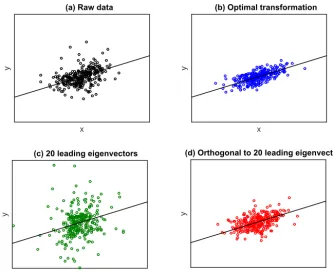
x

y

(a) Raw data

x

y

(c) 20 leading eigenvectors

x

y

(d) Orthogonal to 20 leading eigenvectors

x

y

(b) Optimal transformation

Figure 2.(a)Scatter plot of one realization of the raw data (y,x) using the simulation test bed of Section 4: the observation vectoryis plotted on the vertical axis and the first column vectorx1of the matrixxis plotted on the horizontal axis.(b)Same as(a)for the transformed

dataTy andTxusing the optimal transformation matrixT=V1−12V0.(c)Same as(b)when using the truncated transformation matrix

Tr =Vr1 −1

2

r V0r on the leading eigenvectors, withr=20.(d)Same as(b)when using the proposed transformation matrixT⊥r =V⊥r V⊥r 0

withr=20.

under a closed form expression:

f :S+

n(R)→Rp,

f(A)=(x0_x−x0_V

AV0_Ax)−1(x0y−x0VAV0_Ay).

(28)

The proof of Eq. (28) is detailed in Appendix A. The pro-posed estimator bβ_r∗of Eq. (15) is therefore obtained by ap-plying the extended functionf defined above, to the known, positive semi-definite matrix6r:

b

β_r∗=f(6r)=(x0x−x0VrV0rx)

−1_(x0_y−x0_V

rV0ry). (29)

4 Simulations and illustration

4.1 Data

We illustrate the method by applying it to surface tempera-ture data and climate model simulations over the 1901–2000 period and over the entire surface of the Earth. For this pur-pose, we use the data described and studied in Ribes and Terray (2012). The temperature observations are based on the HadCRUT3 merged land–sea temperature data set (Bro-han et al., 2006). The simulated temperature data used to estimate the response patterns are provided by results from the CMIP5 archive arising from simulations performed with

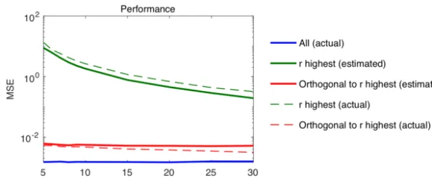
Figure 3.Performance results on simulated data: MSE of several estimators ofβ(vertical axis) as functions of the number of eigenvectors r(horizontal axis) assumed to be reliably estimable from control runs: conventional estimatorβbrcomputed based on estimated eigenvectors (thick green line) withN=30, and based on the true eigenvectors (light green line); proposed orthogonal estimatorβb_r∗computed based on estimated eigenvectors (thick red line) withN=30, and based on the true eigenvectors (light red line); GLS estimator computed based on the true value of the covariance6(thick blue line).

4.2 Performance on simulated data

This section evaluates the performance of the estimators de-scribed above, by applying it to simulated values of y ob-tained from the linear regression equation y=xβ+ν as-sumed by the model of Eq. (1), where the noiseνis simulated from a multivariate Gaussian distribution with covariance6 and whereβ=(1,1)0is used. This setting thus assumes that xis known exactly, therefore it does not include the EIV sit-uation prevailing in Eq. (20) and in Sect. 3.3 wherexis mea-sured with an error.

The use of simulated rather than real data aims at veri-fying that our proposed estimator performs correctly, and at comparing its performance with the conventional procedure, a goal which requires the actual values of β to be known. A sample ofN=30 control runs was also simulated from a multivariate Gaussian distribution with covariance6, and the r leading eigenvectors and eigenvalues were estimated from these control runs.

Figure 2 shows scatter plots of one realization of the data (x,y) under this test bed, for the raw data (x,y) as well as for the transformed data (Tx,Ty), when using the three main transformations considered above: the optimal transforma-tionT=V1−12V0which assumes a fully known covariance

6; the truncated transformation matrix Tr=Vr1 −1

2 r V0r on

the r leading eigenvectors, with r=20, and the proposed projection matrix T⊥_r =V⊥_rV⊥_r 0 on the orthogonal to the r leading eigenvectors, again withr=20. Figure 2 allows the behavior of these transformations to be visualized. Firstly, the benefit of the optimal transformationT=V1−12V0 ap-pears clearly, as it greatly enhances the signal. Secondly, it is also apparent that the standard truncated transformation us-ing therleading eigenvectors fails to enhance the signal, ac-tually leading to a cloud of points which is more noisy than the original raw data. In contrast, the proposed transforma-tion on the orthogonal to the r leading eigenvectors

accu-rately captures part of the signal enhancement produced by the optimal transformation.

The conventional estimatorβbrand the proposed estimator b

β_r∗of Eq. (15) were both derived based on therleading es-timators estimated from theN control runs. Then, these two estimators were derived again, this time using the true values of ther leading eigenvectors, for comparison. Finally, the GLS estimator of Equation (1) was derived based on the true value of the covariance6. The performance of each five es-timators ofβthus obtained was evaluated based on average mean squared error (MSE)PJ

j=1(bβj−β)0(bβj−β)/N, where

j=1, . . ., J denotes the simulation number and J=1e4. These calculations were repeated for several values ofr rang-ing from 5 to 30. Results are plotted in Fig. 3. They show an important gap in MSE between the proposed estimator and the conventional approach with the former exceeding the latter by a factor of 1000 forr=5, decreasing to 80 for r=30. This gap suggests a substantial benefit of usingβb_r∗ and strongly emphasizes the relevance of this approach com-pared to the conventional one.

When comparing the performance ofβb ∗

r using estimated

vs. actual values of therleading eigenvectors, a slight bene-fit of using actual values is found. This benebene-fit increases with r, as eigenvectors with lower eigenvalues tend to be more difficult to estimate. In contrast, when comparing the perfor-mance ofβbrusing estimated vs. actual values of therleading

eigenvectors, a slight benefit of using the estimated values is found. This superiority of the estimated, and thus incorrect, values may seem surprising at first, but is in fact natural and in line with our main point. Indeed, it can be explained by the fact that the estimated leading eigenvectorsbVr match to

a large extent withVr but also span to some extent the true

orthogonal subspaceV⊥

r , which, according to our main point

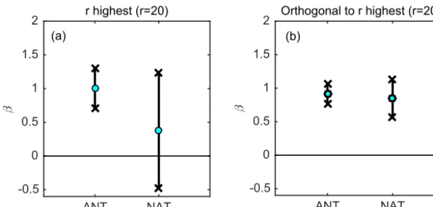
ANT NAT

β

-0.5 0 0.5 1 1.5

2 r highest (r=20)

ANT NAT

β

-0.5 0 0.5 1 1.5

2 Orthogonal to r highest (r=20) (b)

(a)

Figure 4.Illustration of temperature data withr=20.(a)Regression coefficientsβANTandβNATestimated using the conventional estimator

b

βr: value of the estimate (green dots) and 95 % confidence interval (thick black lines).(b)Same as(a)under the proposed estimatorβb_r∗.

thus performs better than its counterpart based on actual val-ues.

4.3 Illustration on real data

The method is finally illustrated by applying it to actual ob-servations of surface temperaturey, with the same regressors x and covariance6 as described above. The observed tem-perature datayis based on the HadCRUT3 merged land–sea temperature data set (Brohan et al., 2006). The method is ap-plied forr=20. Further, we use a number of control runs N that is small compared to n, which is a common situa-tion, even though we have access under the present test bed to 374 control runs. Thus,N=30 control runs are randomly selected from the 374 control runs available and the eigen-vectors are estimated from these 30 runs. For the inference ofβand confidence intervals, we use the solution described in Sect. 3.2 which consists of using Eq. (23) to derive an es-timate ofβand Eq. (25) to derive a confidence interval. Re-sults are shown in Fig. 4. For the scaling factor corresponding to anthropogenic forcings, both methods yield an estimate which is close to 1 and significantly positive. However, the level of uncertainty obtained with the proposed estimator is 3 times smaller than when using the conventional method. An even wider uncertainty gap is observed for the coefficient corresponding to natural forcings. In this case, the confidence interval includes zero under the conventional approach, but it does not under the proposed orthogonal approach. However, as already stated in Sect. 3, a caveat in the latter result is that the uncertainty quantification procedure used here has not been evaluated in detail, and thus we do not know for sure that the obtained uncertainty estimate is well calibrated.

5 Conclusions

We have introduced a new estimator of the vectorβ of lin-ear regression coefficients, adapted to the context where only the r leading eigenvectors of the noise’s covariance 6 are

known, which is an assumption often relevant in climate change attribution studies. General considerations have first shown that when the covariance is known, its most relevant eigenvectors for projection are those trading off the small-est possible eigenvalue with the bsmall-est possible alignment to the signal. The optimal direction is thus associated in general with the smallest eigenvalues, not with the highest ones. Our proposed estimator builds upon this finding and is based on projecting the data on a subspace which is orthogonal to the rleading eigenvectors.

When applied on a simulation test bed that is realistic with respect to D&A applications, we find that the proposed esti-mator outperforms the conventional estiesti-mator by several or-ders of magnitude for small values ofr. Our proposal is thus prone to significantly affect D&A results by decreasing the estimated level of uncertainty.

Substantial further work is needed to evaluate the perfor-mance of the proposed uncertainty quantification, in partic-ular in an EIV context. Such an evaluation was beyond the scope of the present work. Its primary focus was to demon-strate that the choice of the leading eigenvectors as a projec-tion subspace is a vastly suboptimal one for D&A purposes; and that projecting on a subspace which is orthogonal to the rleading eigenvectors yields a significant improvement.

Appendix A: Proof of equation (28)

Let A∈S+₍

R) be a non-invertible positive matrix. Denote

1Athe matrix of non-zero eigenvalues ofA,VAthe matrix of eigenvectors associated with 1A and V⊥_A the matrix of eigenvectors associated with the eigenvalue zero. Forε >0, we have the following:

(A+εI)−1 _=(V

A1AV0_A+εI)−1 =(VA1AV0_A+εV⊥_AV⊥_A

0

+εVAV0_A)−1

=

VA(1A+εI)V0_A+εV⊥_AV⊥_A

0−1

=VA(1A+εI)−1V0A+ 1

εV ⊥

AV

⊥

A

0

.

(A1)

Therefore,

f(A+εI)=

x0VA(1A+εI)−1V0Ax+ 1 εx

0_V⊥

AV

⊥

A

0

x −1

x0VA(1A+εI)−1V0Ay+ 1 εx

0_V⊥

AV

⊥

A

0

y

=x0VABεV0Ax+x

0

V⊥_AV⊥_A0x

−1

x0VABεV0Ay+x

0

V⊥_AV⊥_A0y, (A2)

withBε=ε(1A+εI)−1. We have limε→0+B_ε=0, hence,

limε→0+ f(A+εI)=

x0_V⊥ AV

⊥ A 0

x

−1 x0_V⊥

AV

⊥

A

0

y =(x0_x−x0_V

AV0_Ax)−1(x0y−x0VAV0_Ay), (A3)

Competing interests. The author declares that there is no con-flict of interest.

Acknowledgements. This work was supported by the ANR grant DADA and by the LEFE grant MESDA. I thank Dáithí Stone, Philippe Naveau and two anonymous reviewers for very useful comments and discussions that helped improve considerably this article.

Edited by: Christopher Paciorek Reviewed by: two anonymous referees

References

Allen, M. and Stott, P.: Estimating signal amplitudes in optimal fin-gerprinting, part i: theory, Clim. Dynam., 21, 477–491, 2003. Allen, M. and Tett, S.: Checking for model consistency in optimal

fingerprinting, Clim. Dynam., 15, 419–434, 1999.

Amemiya, T.: Advanced Econometrics, Harvard University Press, 1985.

Bell, T. P.: Theory of optimal weighting of data to detect climate change, J. Atmos. Sci., 43, 1694–1710, 1986.

Brohan, P., Kennedy, J., Harris, I., Tett, S., and Jones, P.: Un-certainty estimates in regional and global observed tempera-ture changes: a new data set from 1850, J. Geophys. Res., 111, D12106, https://doi.org/10.1029/2005JD006548, 2006. Casella, G. and Berger, R. L.: Statistical Inference, Duxbury, 2nd

Edition, 2008.

Fuller, W. A.: Measurement Error Models, John Wiley, New York, 1987.

Hannart, A.: Integrated Optimal Fingerprinting: Method description and illustration, J. Climate, 29, 1977–1998, 2016.

Hannart, A., Ribes, A., and Naveau, P.: Optimal fingerprinting un-der multiple sources of uncertainty, Geophys. Res. Lett., 41, 1261–1268, https://doi.org/10.1002/2013GL058653, 2014. Hasselmann, K.: On the signal-to-noise problem in atmospheric

re-sponse studies, in: Meteorology of tropical oceans, edited by: Shaw, D. B., 251–259, Royal Meteorological Society, London, 1979.

Hegerl, G. C. and North, G. R.: Comparison of statistically optimal methods for detecting anthropogenic climate change, J. Climate, 10, 1125–1133, 1997.

Hegerl, G. and Zwiers, F.: Use of models in detection and attri-bution of climate change, WIREs Clim Change, 2, 570–591, https://doi.org/10.1002/wcc.121, 2011.

Hegerl, G. C., von Storch, H., Hasselmann, K., Santer, B. D., Cubasch, U., and Jones, P. D.: Detecting greenhouse gas induced climate change with an optimal fingerprint method, J. Climate, 9, 2281–2306, 1996.

Hegerl, G. C., Zwiers, F. W., Braconnot, P., Gillett, N. P., Luo, Y., Marengo Orsini, J. A., Nicholls, N., Penner, J. E., and Stott, P. A.: Understanding and Attributing Climate Change, in: Cli-mate Change 2007: The Physical Science Basis. Contribution of Working Group I to the Fourth Assessment Report of the Inter-governmental Panel on Climate Change, edited by: Solomon, S., Qin, D., Manning, M., Chen, Z., Marquis, M., Averyt, K. B., Tig-nor, M., and Miller, H. L., Cambridge University Press, Cam-bridge, United Kingdom and New York, NY, USA, 2007. Lott, F. C., Stott, P. A., Mitchell, D. M., Christidis, N., Gillett, N. P.,

Haimberger, L., Perlwitz, J., and Thorne, P. W.: Models versus radiosondes in the free atmosphere: A new detection and attri-bution analysis of temperature, J. Geophys. Res.-Atmos., 118, 2609–2619, https://doi.org/10.1002/jgrd.50255, 2013.

Min, S., Zhang, X., and Zwiers, F. W.: Human-Induced Arctic Moistening, Science, 320, 518–520, 2008.

Naderahmadian, Y., Tinati, M. A., and Beheshti, S.: Generalized adaptive weighted recursive least squares dictionary learning, Signal Process., 118, 89–96, 2015.

North, G. R. and Stevens, M. J.: Detecting climate signals in the surface temperature record, J. Climate, 11, 563–577, 1998. North, G. R., Bell, T. L., Cahalan, R. F., and Loeng, F. J.: Sampling

errors in the estimation of empirical orthogonal functions, Mon. Weather Rev., 110, 600–706, 1982.

Poloni, F. and Sbrana, G.: Feasible generalized least squares esti-mation of multivariate GARCH(1,1) models, J. Multivar. Anal., 129, 151–159, 2014.

Ribes, A. and Terray, L.: Regularised Optimal Fingerprint for at-tribution. Part II: application to global near-surface temperature based on CMIP5 simulations, Clim. Dynam., 41, 2837–2853, https://doi.org/10.1007/s00382-013-1736-6, 2012.

Ribes, A., Planton, S., and Terray, L.: Regularised Opti-mal Fingerprint for attribution. Part I: method, proper-ties and idealised analysis, Clim. Dynam., 41, 2817–2836, https://doi.org/10.1007/s00382-013-1735-7, 2012.