Study and the effects of ignition timing on gasoline engine performance and emissions

ORIGINAL PAPER

Study and the effects of ignition timing on gasoline engine

performance and emissions

J. Zareei&A. H. Kakaee

Received: 1 November 2011 / Accepted: 31 March 2013 / Published online: 25 April 2013 #The Author(s) 2013. This article is published with open access at SpringerLink.com

Abstract

IntroductionIgnition timing, in a spark ignition engine, is the process of setting the time that an ignition will occur in the combustion chamber (during the compression stroke) relative to piston position and crankshaft angular velocity. Setting the correct ignition timing is crucial in the perfor-mance and exhaust emissions of an engine.The objective of the present work is to evaluate whether variable ignition timing can be effect on exhaust emission and engine perfor-mance of an SI engine.

Method For achieving this goal, at a speed of 3400 rpm, the ignition timing has been changed in the range of 41° BTDC to 10° ATDC and for optimize operation, ignition timing has been designed at wide-open throttle and at last, the performance characteristics such as pow-er, torque, BMEP, volumetric efficiency and emissions are obtained and discussed.

Results The results show optimal power and torque is achieved at 31°CA before top dead centre and volumetric efficiency, BMEP have increased with rising ignition timing. O2, CO2, CO has been almost constant, but HC with

advance of ignition timing increased and the lowest amount NOxis obtained at 10 BTDC.

ConclusionsIn conclusion, it obtained that ignition timing can be used as an alternative way for predicting the perfor-mance of internal combustion engines. Also engine speed and throttle position were all found to significantly influence performance in this engine.

Keywords Ignition timing . Performance . Emission . Spark ignition engine

1 Introduction

The performance of spark ignition engines is a function of many factors. One of the most important ones is ignition timing. Also it is one of the most important parameters for optimizing efficiency and emissions, permitting combustion engines to conform to future emission targets and standards [1]. Since the advent of Otto’s first four stroke engine, the development of the spark ignition engine has achieved a high level of success. In the early years, increasing engine power and engine working reliability were the principal aims for engine designers. In recent years, however, ignition timing has brought increased attention to development of advanced SI engines for maximizing performance [2,3].

Chan and Zhu worked on modeling of in-cylinder ther-modynamics under high values of ignition retard, in partic-ular the effect of spark retard on cylinder pressure distribution. In- cylinder gas temperature and trapped mass under varying spark timing conditions were also calculated [4]. Soylu and Gerpen developed a two zone thermodynam-ic model to investigate the effects of ignition timing, fuel composition, and equivalence ratio on the burning rate and cylinder pressure for a natural gas engine [5]. Burning rate analysis was carried out to determine the flame initiation period and the flame propagation period at different engine operating conditions [5].

A zero-dimensional thermodynamic cycle model with two zone burnt/unburned combustion model, mainly based on Ferguson’s and Krikpatrick work [6], was developed to predict the cylinder pressure, work done, heat release, en-thalpy of exhaust gas, and so forth. The zero-dimensional model is based on the first law of thermodynamics in which an empirical relationship between the fuel burning rate and crank angle position is established.

Now a day sustaining a clean environment has become an important issue in an industrialized society. The air pollution caused by automobiles and motorcycles is an important

J. Zareei (*)

:

Department of Automotive, Iran University of Science and Technology, Tehran, Iran

environmental problem to be solved. For this purpose, find-ing new alternative energy sources in place of petroleum in internal combustion engines is becoming a necessity more than ever.

2 Test engine

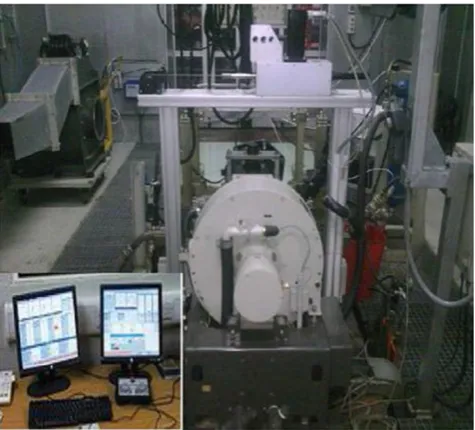
Facilities to monitor and control engine variables (such as: engine speed, engine load, water and lube oil temperatures, fuel and air flows etc.) are installed on a fully automated test bed, experimental standard SI engine, located at the Iran Khodro Company Laboratory. The first set of performance data was taken varying timing angle, the intake manifold pressure was 100Kpa and equivalence was held at unity. The specifications of the test engine are given in Table1.

The engine is mounted on a fully automated test bed and coupled to a Schenck W130 eddy current dynamometer, having load absorbing and motoring capabilities. There is one electric sensor for speed and one for load, with these signals fed to indicators on the control panel and to the controller. Via knobs on the control panel, the operator can set the dynamometer to control speed or load. There is also a capability of setting the ignition timing from a switch on the control panel. The coolant and lube oil circulation is achieved by electrically driven pumps, with the temperature controlled by water fed heat exchangers. Heaters are used to maintain the oil and coolant temperatures during warm up and light load conditions. Figure1is the control panel and test engine on dynamometer.

3 Method

3.1 Exhuastgas analisis aparatus

The exhaust gas analysis apparatus consists of a series of analyzers for measuring soot, NOx, CO and total unburned

Hydrocarbons (HC). The smoke (soot) level in the ex-haust gas was measured with an ‘AVL Di Gas’ the readings of which are provided as Hart ridge units (% opacity) or equivalent smoke (soot) density (milligrams of soot per cubic meter of exhaust gases). The nitrogen oxides concentration in ppm (parts per million, by vol-ume) in the exhaust was measured with a ‘Signal’ Series-4000 analyzer and was fitted with a thermostati-cally controlled heated line.

3.2 Experimental errors

No physical quantity can be measured with perfect certainty; there are always errors in any measurement. This means that if we measure some quantity and, then, repeat the measure-ment, we will almost certainly measure a different value the second time.

However, as we take greater care in our measurements and apply ever more refined experimental methods, we can reduce the errors and, thereby, gain greater confidence that our measurements approximate ever more closely the true value [7].

3.2.1 Combining errors in calculations

When several measurements are taken and combined in formulas, the resultant error will be a combination of indi-vidual errors. Although errors may cancel, we must calcu-late the maximum possible error assuming that errors are additive [8,9].

First convert absolute errors to % errors, The maxi-mum possible error is determined by adding the %

Table 1 Engine specifications

Engine type TU3A

Number of strokes 4

Number of cylinders 4

Cylinder diameter (mm) 75

Stroke (mm) 77

Compression ratio 10.5:1

Maximum power (kW) 50

Maximum Torque (NM) 160

Maximum speed (rpm) 6500

Displacement (cc) 1360

Fuel 97-octane

errors together, If a reading is raised to a power in a calculation, then the % error for that part is the power times the % error. Generally, errors can be divided into two broad and rough but useful classes: systematic and random.

Systematic errors are errors which tend to shift all mea-surements in a systematic way so their mean value is displaced. This may be due to such things as incorrect calibration of equipment, consistently improper use of equipment or failure to properly account for some effect [10].

Sources of systematic errors are external effects which can change the results of the experiment, but for which the corrections are not well known. In sci-ence, the reasons why several independent confirmations of experimental results are often required (especially using different techniques) is because different apparatus at different places may be affected by different

system-atic effects. So should be considered errors of apparatus before testing.

3.2.2 Calculation combined error

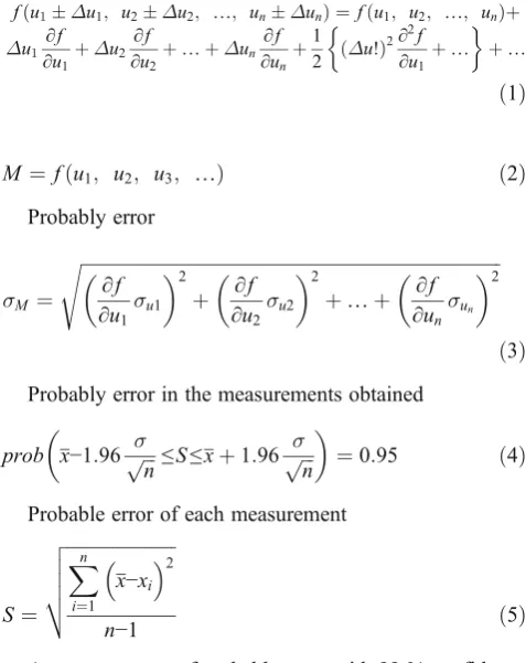
Rate of probable error in each means obtain from combina-tion errors of each part. Assuming M isu1, u2, …un

inde-pendent variable n function of quantity [11,12]

f uð 1Δu1; u2Δu2; …; unΔunÞ ¼f u1ð ; u2; …; unÞþ

Δu1_∂∂f u1þΔu2

∂f

∂u2þ…þΔun

∂f

∂unþ 1

2 ðΔu!Þ

2∂2f

∂u1þ…

þ…

ð1Þ

M ¼f uð 1; u2; u3; …Þ ð2Þ

Probably error

σM¼

ffiffiffiffiffiffiffiffiffiffiffiffiffiffiffiffiffiffiffiffiffiffiffiffiffiffiffiffiffiffiffiffiffiffiffiffiffiffiffiffiffiffiffiffiffiffiffiffiffiffiffiffiffiffiffiffiffiffiffiffiffiffiffiffiffiffiffiffiffiffiffiffiffiffiffiffiffiffiffiffiffiffiffiffiffiffiffiffiffiffiffiffi ∂f

∂u1σu1

2

þ _∂∂f u2σu2

2

þ…þ _∂∂f unσun

2

s

ð3Þ

Probably error in the measurements obtained

prob x−1:96 σffiffiffi

n

p ≤S≤xþ1:96 σffiffiffi

n p

¼0:95 ð4Þ

Probable error of each measurement

S ¼

ffiffiffiffiffiffiffiffiffiffiffiffiffiffiffiffiffiffiffiffiffiffiffiffi

Xn

i¼1 x−xi

2

n−1

v u u u t

ð5Þ

Average amount of probable error with 99 % confidence

q¼ 2:54ffiffiffiS n

p ð6Þ

Table 2 Accuracy of measurements and uncertainty of computed

results

Measurements Accuracy

Soot density ±1 mg/m3

NOx ±5 ppm

CO ±3 ppm

HC ±2 ppm

Time ±0.5 %

Speed ±2 rpm

Torque ±0.1 N m

Computed results Uncertainty

Fuel volumetric rate ±1 %

Power ±1 %

Specific fuel consumption ±1.5 %

Efficiency ±1.5 %

Fig. 2 The relation between

Average amount of probable error with 95 % confidence

q¼ 1:96ffiffiffiS n

p ð7Þ

Once there are some experimental measurements, they usually combine according to some formula to arrive at a desired quantity. To find the estimated error for a calculated result one must know how to combine the errors in the input quantities. The simplest procedure would be to add the errors. This would be a conservative assumption, but it overestimates the uncertainty in the result. Clearly, if the errors in the inputs are random, they will cancel each other at least some of the time. If the errors in the measured quantities are random and if they are independent can be obtained from a few simple formulas. In this research, average amount of probable error with 99 % confidence have obtained.

3.2.3 Condition and parameters tested-experimental procedure

The series of tests are conducted using variation of ignition timing with the engine working at a speed of 3400 rpm at a

ignition timing (advance) of 41 crank angle before TDC and at full load. Owing to the differences among the calorific values and oxygen content of the fuels tested, the compar-ison must be effected at the same engine brake mean effec-tive pressure, i.e. load, and not at air/fuel ratio. in this also tests are considered accuracy of measurements and the be-low table shoes accuracy of measurements and uncertainty of computed results.

In each test, volumetric fuel consumption, exhaust smok-iness and exhaust regulated gas emissions, such as Nitrogen Oxides (NOx), Carbon monoxide (CO) and total unburned Hydrocarbons (HC), are measured. From the first measure-ment, specific fuel consumption and brake thermal efficien-cy are computed using the sample density and lower calorific value. Table2shows the accuracy of the measure-ments and the uncertainty of the computed results of the various parameters.

4 Results and discussion

The first adjust of performance data was taken varying throttle position. By changing the Position of the throttle,

Fig. 3 The relationship

between exhaust temperature and In cylinder peak pressure versus ignition timing-wide open throttle; equivalence ration of one

Fig. 4 The relationship

the intake manifold pressure was varied to 100 kPa- on position wide-open throttle. Speed was held at 3400 RPM and equivalence ratio was held at unity.

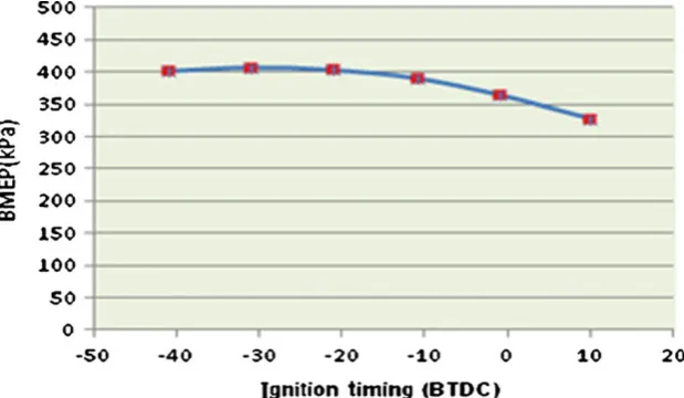
The results show that Brake Mean Effective Pressure (BMEP) tends to increase with ignition timing till 31° Before Top Dead Centre (BTDC) and then drop off. Best performance will be achieved when he greatest ignition 31° BTDC. If ignition timing isn’t advance enough, original portion of the maximum pressure will creative in the expand stroke and in this case we lose useful efficiency and decreasing performance.

The maximum BMEP is at an ignition timing 31°BTDC minimum advance for Maximum Brake Torque (MBT) is defined as the smallest advance that achieves 99 % of the maximum power.

It should be noted that MBT will vary with both throttle position and engine speed under more throttle condition; the density of charge in the cylinder in less dense mixtures, a not very large ignition timing advance will be required. In this case ignition occurs and gives a suitable performance (Fig. 2).

The above figure shows that Indicated Mean Effective Pressure (IMEP) tends to increase with ignition timing ad-vance between 21 and 41° BTDC. It is expected that IMEP should increase with timing angle advance to a point, and then drop off. Best performance will be achieved when the greatest portion of the combustion takes place near top dead center. If the ignition timing is not advanced enough, the piston will already be moving down when much of the combustion takes place. In this case we lose the ability to expand this portion of the gas through the full range, decreasing performance. If the ignition timing is too advanced, too much of the gas will burn while the piston is still rising. The work that must be done to compress this gas will decrease the net work produced. These competing effects cause there to be a maximum in the IMEP as a function of ignition timing advance.

As is evident in Fig. 3 the peak pressure increases with increasing ignition timing before top dead center. Maximum pressure would be reached if all of gas were burned by the time the piston reached TDC. But pressure decreases with less advanced ignition timing because; gas doesn’t burn complete-ly until the piston is on its way down on the expansion stroke.

Fig. 5 The relationship

between BSFC and ignition timing at 3400 RPM and equivalence ratio of unity

Fig. 6 The relationship

between O2and HC

The Above figure also shows that the exhaust tempera-ture decrease with close to TDC and ATDC. IMEP repre-sents the work done on the piston. The exhaust gas temperature represents the enthalpy of the exhaust gas for ideal gases. The enthalpy is a function of temperature only and energy released by combustion of fuel must go into expansion work. The temperatures of the exhaust gas also decrease if energy is to be conserved (Fig.4).

The results show that BMEP increased with ignition timing advance. This expected that BMEP decrease with closing ignition time to top dead center. If the ignition is not advanced enough, the piston will already be moving down when much of the combustion take place. In this case we lose the ability to expend this portion of the gas and decreasing performance. If the ignition is too advance, much portion of gas will burn while the piston is still rising; the work that must be done to compress this gas will decrease the net work produced. Also, results show that maximum BMEP is between−21° to 41° and the date has a maximum BMEP at ignition timing at 31°BTDC.

Figure5 Shows that Brake Specific Fuel Consumption (BSFC) tend to improve with increase of ignition timing

before top dead centre. It should be noted that when BMEP increase, BSFC follows inversely.

Figure6shows O2and HC concentration as a function of

timing angle. Advance timing angle causes higher in cylin-der peak pressure. This higher pressure pushes more of the fuel- air mixture into crevices (most significantly the space between the piston crown and cylinder walls) where the flame is quenched and mixture is left unburned. Additionally, the temperature late in the cycle, when the mixture comes out of these crevices, is lower at more advance ignition timing. The later temperature means that the hydrocarbons and oxygen do not react. This increase the concentration of oxygen in the exhaust and unburned hydrocarbons.

In above figure carbon monoxide, oxygen and carbon dioxide concentration change very little with ignition timing in the range studied (Fig.7).

In here, the equivalence ratio was held constant and at ratio of unity, so there was enough oxygen to react most of carbon to CO2. CO concentration increased and CO2concentration

decreased when there isn’t enough oxygen. Some carbon monoxide does appear in the exhaust due to frozen equilibri-um concentration of CO, O2and CO2.

Fig. 7 The relationship

between O2, CO and HC

concentration versus ignition timing intake manifold pressure of 100 kPa and equivalence ratio of unity

Fig. 8 The relationship

Figure shows NO concentration in the exhaust gas versus ignition timing. NO formation is function of temperature. With advancing the ignition timing, the in- cylinder peak pressure increase. The ideal gas law tells that increase in peak pressure must correspond to an increase in peak tem-perature, and higher temperature causes the NO concentra-tion to be higher (Fig.8).

The results show that power tends to increase with spark advance between 17 and 35°CA BTDC. It is expected that power should increase with spark advance to a point, and then drop off. Best performance will be achieved when the greatest portion of the combustion takes place near top dead centre. If the spark is not advanced enough, the piston will already be moving down when much of the combustion takes place. In this case, we lose the ability to expand this portion of the gas through the full range, decreasing perfor-mance. If ignition is too advanced, too much of the gas will burn while the piston is still rising. As a result, the work that must be done to compress this gas will decrease the net work produced. These competing effects cause there to be a maximum in the power as a function of spark advance.

Also it shows that the torque increases with increasing ignition advance. This is due to increasing pressure in the compression stroke and consequently more net work is produced. It is necessary to mention that by further increase in spark advance, torque will not rise largely due to in-cylinder peak pressure during compression period and a decrease of pressure in expansion stroke. For this reason, determining the optimum ignition timing is one of the most important characteristics for an SI engine (Fig.9).

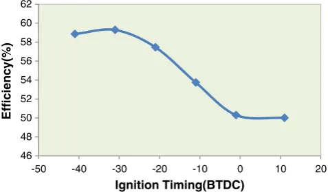
Figure10 presents the predicted results of thermal ciency in comparison with experimental data. Thermal effi-ciency is work-out divided by energy-in. It can be seen that the net work increases with rising ignition advance to a point, and then reduces slightly. This is due to increasing friction at high values of ignition advance and therefore reducing net work. According to Fig.6, the highest amount of the net work occurs at 31°CA BTDC.

5 Conclusion

The aim of this paper was effects of ignition timing of a spark- ignition engine using different initial timing and engine speeds on engine performance by experimental. The overall results show that ignition timing can be used as an alternative way for predicting the performance of internal combustion engines. In this paper, the best results were obtained at 31°BTDC for 3400RPM. Also engine speed and throttle position were all found to significantly influence performance in this engine. Volumetric efficiency, BMEP have increased with rising ignition timing. HC with advance of ignition timing increased, O2, CO2, CO has been

almost constant and the lowest amount NOx is obtained at 10°BTDC. For future work, it recommended ignition timing and valve timing be controlled together and change throttle position in different speeds.

70 75 80 85 90 95 100 105 110 115 120

20 25 30 35 40 45 50

-50 -40 -30 -20 -10 0 10 20

Torque(Nm)

Po

w

e

r(

K

w

)

Ignition timing(BTDC)

Power

Torque

Fig. 9 The relationship

between power and torque versus ignition timing

46 48 50 52 54 56 58 60 62

-50 -40 -30 -20 -10 0 10 20

Efficiency(%)

Ignition Timing(BTDC)

Open AccessThis article is distributed under the terms of the Creative Commons Attribution License which permits any use, distribution, and reproduction in any medium, provided the original author(s) and the source are credited.

References

1. Golcu M, Sekmen Y, Salman MS (2005) Artificial neural-network based modeling of variable valve-timing in a spark-ignition engine. Applied Energy 81:187–197

2. Chan SH, Zhu J (2001) Modeling. Int J Therm Sci 40(1):94– 103

3. Soylu S, Van Gerpen J (2004) Development of empirically based burning rate sub-models for a natural gas engine. Energy Convers Manage 45(no. 4):467–481. doi:10.1016/S0196-8904(03)00164-X 4. Chan SH, Zhu J (2001) Modeling of engine in-cylinder thermody-namics under high values of ignition retard. Int J Therm Sci 40(1):94–103

5. Soylu S, Van Gerpen J (2004) Development of empirically based burning rate sub-models for a natural gas engine. Energy Convers Manage 45(4):467–481

6. Ferguson CR, Krikpatrick AT (2001) Internal combustion engines-Applied thermo sciences. Wiley, New York

7. Choia GH, Chungb YJ, Hanc SB (2005) Performance and emis-sions characteristics of a hydrogen enriched LPG internal combus-tion engine at 1400 rpm. Int J Hydrogen Energy 30:77–82 8. Teter WD (2007) Instruments and Controls Professor, Department

of Civil Engineering, College of Engineering, University of Dela-ware. Section 16

9. UKAS publication M 3003 (1997) The expression of uncertainty and confidence in measurement Edition 1, December

10. Harrison MD (2011) Error analysis in experimental physical science 11. Taylor JR (1997) An introduction to error analysis: the study of uncertainties in physical measurements, 2nd Edition, University Science Books