J. Sens. Sens. Syst., 1, 5–27, 2012 www.j-sens-sens-syst.net/1/5/2012/ doi:10.5194/jsss-1-5-2012
©Author(s) 2012. CC Attribution 3.0 License.
Geoscientific
Instrumentation
Methods and
Data Systems
Discussions
Geoscientific
Instrumentation
Methods and
Data Systems
Open Access
Web Ecology
Open Access
Open
Access
JSSS
Journal of Sensors and Sensor SystemsF
eature
Ar
ticle
Compensation method in sensor technology:
a system-based description
V. Schulz1, G. Gerlach1, and K. R¨obenack2
1Solid-State Electronics Laboratory, Technische Universit¨at Dresden, 01062 Dresden, Germany 2Institute of Control Theory, Technische Universit¨at Dresden, 01062 Dresden, Germany
Correspondence to: V. Schulz ([email protected])
Received: 24 May 2012 – Revised: 17 July 2012 – Accepted: 23 July 2012 – Published: 3 August 2012
Abstract. In measurement science and engineering, the method of compensation plays a decisive role and is widely used in practical applications, in particular for sensors and measurement systems, where high accuracy is required. However, a general theoretical system description of this method with particular respect to figures of merit in sensor technology does not exist yet. Nevertheless, this is important for a real understanding of the system’s structure and its properties and would facilitate prospective sensor design. Within this work, we pro-vide a general system-based description and comparison of both the compensation and the deflection method. Based on a general sensor model and selected transfer functions, which cover most sensor types, important sensor properties like static deviations in sensitivity, long-term drift effects, response time, output signal char-acteristics as well as nonlinearities and hysteresis are studied in a systematic fashion for both measurement methods. In the case of a compensation method, the core sensor element is part of a controlled closed-loop system, leading to different system properties compared to an open-loop sensor operated in deflection method. The influence of linear standard controllers, which are widely used in industrial measurement and control sys-tems, is studied with respect to the sensor properties. In the conclusions we will summarize which controller type is appropriate for the attainment of a specifically targeted sensor behavior.
1 Introduction
“The history of science is the history of measurement” (Cat-tell, 1893). Even though claimed by a psychologist in the late 19th century, the validity of this statement in the fields of sci-ence and engineering is unchallenged. Measurement technol-ogy has explosively developed, and is still immensely grow-ing, with an almost unmanageable diversity of complex sen-sors and measurement systems. Despite this variety and in-cessant new developments, the improvement of existing sen-sor concepts has always been of high interest. In almost every field of sensors, improvements regarding accuracy, repeata-bility, drift and hysteresis compensation, error proneness, re-sponse time and many more are highly desirable, regardless of the specific sensor principle. Usually, the sensor proper-ties of a specific sensor depend on the transducer principle, the sensor material properties and the measurand. In general, sensors can be operated using different measurement
meth-ods (ISO/IEC Guide 99, 2007). Nowadays, most sensors use the deflection method where the sensor output signal is a direct measure of the input signal. This method comprises the lowest demand in terms of system complexity, but on the other hand the sensor output signal is directly determined by the sensor properties, leading to a pre-determined, but often insufficient sensor performance for specific applications.
Fgravity
0
measuring quantity
(e.g. force
F
)
null indicator
Ds
0 Ds = 0
actuator
(a) (b)
Fcounter=-Fgravity
Figure 1.Simplified schematic illustration of the principle of oper-ation of (a) the deflection method and (b) the compensoper-ation method. The spring represents an arbitrary transducer, whereas the mass of the weight generally represents the input signal.
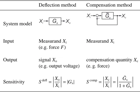
Table 1. Elementary comparison between deflection method and compensation method in measurement.
Deflection method Compensation method
System model Xi Gs Xo
Xi - Gs Xc
~
Input Measurand Xi Measurand Xi
(e.g. force F)
Output signal Xo compensation quantity Xc
(e.g. output voltage) (e. g. force)
Sensitivity Sdefl=
Xo Xi =
|Gs| Scomp=
Xc Xi =
˜ Gs
1+G˜s
almost irrespective of the sensor principle. However, the ap-plicability of this method implies the existence of an actu-ator unit (Fig. 1) which is able to physically generate the compensation quantity. In this method, the actual sensor out-put signal is measured, subtracted from a reference value, and the difference is fed back to the sensor input via a con-troller/actuator unit, until the difference between output sig-nal and reference value reaches zero. Thus, the static sen-sor output signal remains constant for changes in the input signal. Nevertheless, the “force” provided by the actuator needed to maintain this balanced state is directly related to the input signal. Compared to the deflection method, which is an open-loop configuration, a sensor operated with the com-pensation method is a closed-loop system. This leads to dif-ferent system properties solely due to the feedback structure as outlined in Table 1. Furthermore, because of the perpet-uation of the balanced “undeflected” state, the sensor prop-erties negligibly contribute to the overall system behavior, leading to smaller measurement uncertainties and hence to better measurement results. Additionally, the properties of the feedback loop can be set and tuned systematically. This is the reason why the compensation method is used in particular in technical applications with high-precision requirements or expanded operation fields, like precision balances (Krause,
2005), AFMs (in constant force mode) (Bhushan, 2005), broadband lambda probes (Bosch GmbH, 2010), hot-wire anemometers (in constant temperature operation) (Finger-son and Freymuth, 1996; Tavoularis, 2005), MEMS-based accelerometers (Che and Oh, 1996; Stuart-Watson and Tap-son, 2004), continous non-invasive blood pressure monitor-ing (Fortina et al., 2006), or even in hydrogel-based sen-sors very recently (Schulz et al., 2011) (see Sect. 2). De-spite the potential benefits of the compensation method in current and future measurement technology, surprisingly, no general theoretical description of the properties of a sensor operated with the compensation method is available. In par-ticular, theoretical considerations concerning the properties of such sensors with respect to particular requirements in sensor technology like high sensitivity, fast response time, robustness against long-term instabilities of the core sensor element (see gs in Fig. 6) do not exist to our knowledge. Mostly, books on measurement science just refer to the com-pensation method very briefly without any theoretical as-pects or mathematical formulations at all (Webster, 1999; Dyer, 2001; Klaassen, 2002; Bakshi and Bakshi, 2009; Pro-fos and Pfeifer, 1994; Hoffmann, 2007; Lerch, 2011) or even ignore it (Gosh, 2009; Niebuhr and Lindner, 2002). How-ever, some authors have shown system-based calculations for a specific application. In the work of Krause (Krause, 2004, 2005), a comparison between the deflection and the compen-sation method specifically applied to a precision balance is accomplished. In Kiencke and Eger (2008), a system-based approach considering selected aspects of the compensation method is outlined briefly. Moreover, the cited references ap-peared in German and are thus not accessible to an interna-tional readership. Hence, a systematic general system-based description with particular respect to important sensor trans-fer functions, sensor behavior, and sensor properties for prac-tical applications cannot be found in the current literature.
current sensors, are proposed. The modified system structure, which results from the feedback for compensation, is shown and the resulting transfer functions are calculated. These transfer functions are systematically analyzed with respect to certain sensor properties mentioned above. The resulting sensor output signal of the compensated sensor is shown in dependence on the controller parameters.
2 Compensation method in current sensor applications
In this section, a very brief review of the use of the compen-sation method in selected current sensor applications shall be given. Mainly, this section is to show that the compensation method can be applied to a broad range of sensor principles. Therefore, selected sensor principles from different fields of application are introduced, and the advantages due to com-pensation are briefly presented. However, a detailed review or extended description of the respective measurement prin-ciples are beyond the scope of this work.
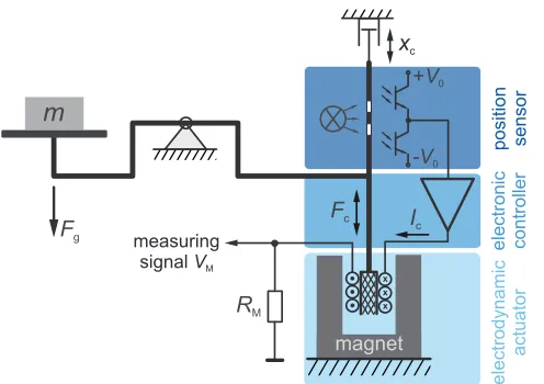
2.1 Electrodynamic precision balance
This balance principle is exceedingly widely used and is ap-plied to measurement problems requiring very high preci-sion. The basic working principle is schematically shown in Fig. 2. If a mass m is applied to the tray, the beam deflects. This deflection xc is detected by an optical position sensor. The coil current Icgenerates the force Fcat the lever and is adjusted by the electronic controller in such a way that the deflection xc in the steady state is zero. Hence, the voltage VMat the resistor RMis proportional to the coil current, and thus, to the applied mass m. The coil current can be set up far more precisely than the beam deflection can be measured. Therefore, weights can be determined with high precision. Furthermore, the beam is quasi-undeflected during the en-tire measuring process. A mechanical deficient or indifferent beam is stabilized by the electronic feedback. Consequently, the mechanical properties of the beam will negligibly affect the measurement process (S¸tefˇanescu, 2011).
2.2 Atomic force microscope in constant force mode The atomic force microscope (AFM) ranks among the most versatile methods for the imaging of nanoscale structures in micro/nano electronics or molecular biology, nanomanipula-tion, and nanoassembly (Bhushan, 2005). Basically, a sharp tip on a flexible cantilever is brought into close proximity to the sample surface, as schematically illustrated in Fig. 3. The resulting interaction between the tip and the sample sur-face causes a deflection d of the cantilever. This deflection is detected by measuring the reflection of a laser spot offof the backside of the cantilever using a four quadrant photo detector. For an undeflected cantilever, ideally, the spot is detected in the center of the detector. A movement of the
m
+V0
-V0
measuring
signal VM
RM
position sensor
magnet
electronic controller
Fc I
c xc
electrodynamic
actuator
x x x
Fg
Figure 2.Basic principle of an electrodynamic precision balance according to Krause (2005) and S¸tefˇanescu (2011).
cantilever leads to a shift of the spot position on the detec-tor. Thus, the detector signal is a direct measure of the can-tilever deflection. Due to the “optical lever”, even small de-flections can be detected reliably. In constant force mode, the detector signal is compared to a reference signal and fed to a controller. The provided controller signal, which leads to a z-movement of the piezo stage zp, is exactly as-sessed such that the cantilever deflection is balanced and the force acting on the cantilever remains constant in the steady state. The controller signal is thus a direct estimate of the surface structure. PI- or PID-controllers are widely used in the feedback loop (Abramovitch et al., 2007). However, also other controller types like Proportional-Double-Integral (PII) or Proportional-Double-Integral-Derivative (PIID) con-trollers have been reported (Abramovitch et al., 2009).
Since the relation between the force acting on the can-tilever and the tip-sample-distance is highly non-linear, the closed-loop configuration enables a reliable detection of the sample surface properties. However, the scan speed is limited by the dynamics of the feedback loop.
2.3 Hot wire anemometer in constant-temperature mode (CTA)
1
2 3
4
x y z
x y z
controller
-referencedeflection photo laser
diode
piezo actuator
surface estimate
z
psample cantilever
d
Figure 3.Basic principle of an atomic force microscope in a closed-loop configuration (constant force mode).
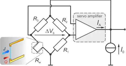
in an increase in resistivity∆Rw, and therefore, in an unbal-anced state of the bridge circuit (∆Vb,0). The difference
voltage∆Vb is amplified by a servo amplifier. The resulting output current IAof the amplifier is fed back to the bridge circuit. This current again induces a temperature increase at the wire probe such that the bridge balance is restored and the wire probe remains at constant temperature at the steady state. In this closed-loop configuration, the amplifier output IAis a function of the dissipated heat from the sensor wire and indirectly of the flow velocity (Fingerson and Freymuth, 1996).
A high gain servo amplifier enables the measurement of rapid flow velocity fluctuations. The cut-off frequency of an anemometer in constant temperature mode can be about three orders of magnitude higher compared to conventional constant current anemometers (Tavoularis, 2005). Due to the constant wire probe temperature, the effect of the thermal in-ertia of the wire is greatly minimized compared to an open-loop system.
2.4 Broadband lambda probe
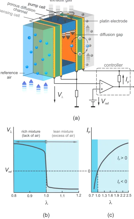
Lambda probes are widely used for oxygen detection and are mainly employed for the measurement of the air/fuel ratio λ in combustion engines in automotive industry, pioneered by Robert Bosch GmbH in the early 1970s. Conventional lambda probes use a galvanic Nernst-cell, composed of a solid electrolyte as oxygen conductor between two platinum electrodes. This cell provides an electrical output voltage Vλ related to the excess oxygen in the exhaust gas. However, with this configuration only a detection of aboutλ=1 is pos-sible. Well above and below this value, the change in the output voltage is only marginal; the transfer characteristics shows a two-step behavior, as shown in Fig. 5b.
Broadband lambda probes – as the name suggests – can operate in a broadλ-range compared to the conventional
de-J
Q
servo amplifier
I0
Rw
R1
R2
R3
I
AD
V
bFigure 4.Basic principle of a hot wire anemometer in constant temperature mode (CTA).
sign (Robert Bosch GmbH, 1994). This broadband configu-ration is schematically shown in Fig. 5a. Here, a sandwich structure comprising a sensing cell, which is identical to the Nernst-cell in the conventional design, a diffusion gap, and a pumping cell are part of a closed-loop control circuit. The exhaust gas is inserted to the diffusion gap via a porous diff u-sion channel, leading to a certain oxygen content inside the diffusion gap and consequently to a certainλ-value. The out-put voltage Vλof the sensing cell directly depends on this λ-value and is compared to the preset reference voltage Vref. The latter is chosen in such a way that it corresponds toλ=1 (≈450 mV). Assumingλ >1 (lean mixture, excess air) in the diffusion gap leads to Vλ<Vref and hence to a voltage dif-ference at the input of the amplifier. This voltage difference results in an output current Ip. This pumping current pumps excess oxygen ions out of the diffusion gap for compensation to maintain a constant air/fuel ratio ofλ=1. Forλ <1 (rich mixture, lack of air) in the diffusion gap, the pumping current has an opposite sign and causes pumping of oxygen ions into the diffusion gap. Thus, an initially imbalanced oxygen con-centration is compensated and theλ-value inside the diff u-sion gap remains constant at the steady state. The magnitude and the sign of the pumping current are a measure ofλ.
With this closed-loop configuration, a broad λ-range 0.7< λ <∞can be detected, whereas∞indicates the oxy-gen concentration of pure air of 21 % (see Fig. 5c). This en-ables expanded areas of application apart from its standard use (Bosch GmbH, 2010).
3 General sensor model with deflection method
3.1 Sensor model
+
-
I
pV
refexhaust gas pump cell
sensing cell
reference air porous dif
fusion channel
platin electrode
diffusion gap
controller
V
l(a)
l
0.8 0.9 1.0 1.1 1.2
rich mixture (lack of air)
lean mixture (excess of air)
Vref
Vl
0
I
Pl
0.7 1.0 1.3 1.6 1.9 2.2 2.5
IP > 0
IP < 0
(b) (c)
Figure 5.(a) Schematic illustration of the core section of a broad-band lambda probe including the feedback control circuit, accord-ing to NGK (2012) (for the sake of simplicity, the heater neces-sary to heat up the probe to the optimal working temperature is not shown in this illustration); general illustration of the transfer char-acteristics of a conventional (b) and a broadband lambda probe (c) according to Bosch GmbH (2010).
is assumed to be an electrical output signal (voltage or cur-rent) according to the general sensor definition, and∗is the convolution operator. Furthermore, we assume the sensor to be a linear time-invariant (LTI) system. The linear dynamic input–output relation of the sensor in the time domain can be completely described by an ordinary linear differential equa-tion of order n (n≥m; n,m∈N) with constant coefficients in the following form:
an dnxo
dtn +an−1 dn−1xo
dtn−1 +· · ·+a1
dxo
dt +a0xo =
bm dmx
i dtm +bm−1
dm−1x i
dtm−1 +· · ·+b1
dxi
dt +b0xi. (1)
x
i(
t
)
g
sx
o(
t
)
X
i(
s
)
G
sX
o(
s
)
x
o(
t
)
=
g
s*x
i(
t
)
X
o(
s
)
=
G
s.X
i(
s
)
(a) (b)
Figure 6.System model of a sensor; (a) in the time domain, (b) in the frequency domain.
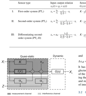
Here, a0, ..., an and b0, ..., bm are constant coefficients which are explicitly determined by the sensor properties. However, in consideration of real sensor systems, basically three instrument types, which mainly cover the transfer char-acteristics of most sensors, can be classified according to their dynamic response as: (I) first-order systems (PT1), (II) second-order systems (PT2), and (III) differentiating second-order systems (PT2-D). Thus, Eq. (1) can be simpli-fied for these three cases. The resulting input–output rela-tions in the time domain are given in Table 2. However, to ob-tain the output characteristics for a given input signal, the de-scription in the time domain requires the solution of the dif-ferential equations. This may result in complicated solution algorithms, especially for more complex systems in closed-loop configuration later on. Moreover, the quantitative inter-pretation of the solution and the extraction of practical con-clusions may be not straightforward due to bulky mathemati-cal expressions. Therefore, the sensor transfer characteristics is transformed from the time domain to the frequency do-main, which enables a powerful method for theoretical sys-tem description (Shinners, 1998). Thus, the sensor can be completely described by its transfer function
Gs(s)= Xo(s)
Xi(s)
=L{gs(t)}=
∞
Z
0
gs(t)e−stdt. (2)
Here,Lis the Laplace operator, and s the complex variable. The sensor transfer functions according to Eq. (2) for the three basic sensor types are given in Table 2. The general sensor coefficients in the input–output relations are substi-tuted by the static sensitivity K and the characteristic time constants T , T1, T2, and T3of the respective system.
Table 2.Sensor classification and assignment of the respective input–output relations and resulting transfer functions as well as common examples for the respective sensor types.
Sensor type Input–output relation Sensor transfer function Examples xo(t)=gs∗xi(t) Gs(s)=Xo(s)/Xi(s)
I: First-order system (PT1) xo=ba0
0·
1
a1 a0dtd+1
·xi K·sT1+1 Temperature sensors
(Fraden, 2010)
II: Second-order system (PT2) xo= b0
a0·
1
a2 a0dt2d2+
a1 a0dtd+1
·xi K·T2 1 1s2+T2s+1
Velocity sensors, accelerometers (Fraden, 2010)
III: Differentiating second- xo=a0· b1dtd
a2 a0dt2d2+
a1 a0dtd+1
·xi K· sT3
T2
1s2+T2s+1 Piezoelectric sensors
order system (PT2-D) (Gautschi, 2002),
pyroelectric sensors (Budzier and Gerlach, 2010)
as
a
oK
f(Xi) G(s)
x
offX
iZ
X
oQuasi-static Dynamic
interference channel measurement channel
Figure 7.General sensor model with measurand Xiand sensor
out-put Xo sub-divided in a quasi-static and a dynamic part and
com-prising a measurement and an interference channel. K intrinsic ideal sensitivity, G(s) normalized sensor transfer function,αssensitivity
coefficient, Z interference quantity altering the ideal sensitivity, f non-linearities in the transfer characteristics, xoff sensor offset,αo
offset coefficient.
static sensor offset xoffis measured as output signal. The sen-sor offset is independent of the input signal, and thus, does not contain information from the measurand. However, the offset is superimposed by Z, and hence, changed by the inter-ference quantity. In most sensors, xoffis primarily altered due to temperature changes. The static sensitivity, the offset and the influence of the interference quantity are additively su-perimposed, and together with the dynamic sensor part, gen-erating the sensor output signal Xo. Note that the order of the static and dynamic sensor part is arbitrary and could be also changed. The sensor behavior can be expressed in a general sensor model as
Xo=[(K+ ∆K)·Xi+(xoff+ ∆xoff)]·G(s), (3)
with
∆K=f+Z·αs (4)
and
∆xoff=Z·αo. (5)
It has to be pointed out that the influence of noise is ne-glected in this model. Based on this sensor model, the effect of the compensation method applied to such a sensor regard-ing the influence of non-linearities, the interference quantity and static sensitivity changes on the sensor output signal are of interest (see Sect. 4).
3.2 Quasi-static sensor behavior
For the description of the quasi-static sensor behavior, we as-sume that all dynamic processes are terminated and that the system is in an equilibrium state (G(s)=1 for s→0). Hence, from Fig. 7 and Eq. (3) it becomes clear that the static sen-sor output signal is basically determined by two parts. One is the static sensor offset ˜xoff=(xoff+ ∆xoff)=(xoff+Z·αo), which is determined by the intrinsic sensor offset xoff and the interference quantity Z, but independent of the input sig-nal Xi. The other part is the sensor sensitivity, which is usu-ally altered by non-linearities and the interference quantity Z as a function of the input signal. According to Eq. (3), the resulting sensitivity can be expressed as the superposi-tion of an ideal constant sensitivity K and a deviasuperposi-tion∆K as ˜K=(K+ ∆K). Here, again two cases have to be consid-ered: (i) a time-independent sensitivity change (∆K= con-stant) and (ii) a time-dependent sensitivity change (drift) (∆K= ∆K(s)). For a time-independent sensitivity change, the interference quantity is constant over time. If one consid-ers small time-independent deviations∆K from the ideal be-havior, the impact of relative systematic deviations∆K on the static sensor output signal can be calculated using a Taylor-series and expressed as a systematic static deviationdefls as
defl
s =
∆Xo∆K,s Xo
= 1
Xo ∂Xo
∂K ·∆K=
∆K
E
h
s
e
ele
visce
=e
el +e
visc Es
e
= eele
(
s
)
s
(
s
)
=
1
E
s
+E
/
h
s
.
=
^
s
+d
s
.
K
e
(
s
)
s
(
s
)
=
1
E
=
^
K
=
const.
(a) (b)
e
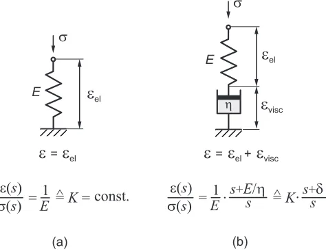
elFigure 8.Mechanical analog and resulting transfer function of a sensor with (a) ideal linear time-independent sensitivity K (no drift) and (b) time-dependent sensitivity change due to viscoelastic mate-rial properties (drift);σmechanical stress,mechanical strain, E Young’s modulus of the elastic spring,ηviscosity of the dashpot.
and is equal to the relative sensitivity change.
The second case of a time-dependent sensor sensitivity (drift) is apparent in many sensor applications and results from time-dependent variations of the interference signal. In this paper, this phenomenon is described by a simple model – known from mechanical sensors – which demonstrates the basic idea but keeps simplicity at the same time. The model originates from a simple spring-dashpot arrangement con-nected in series (Maxwell-model), as illustrated in Fig. 8. This mechanical model represents relaxation effects in spring elements under load due to viscoelastic material properties. The resulting transfer function is used to describe linear drift effects irrespectively of any specific sensor principle. In the frequency domain, ˜K can generally be described as
˜
K(s)=K·s+δ
s , (7)
whereδ is a variable drift rate. Although we consider the static sensor behavior in this section, the phenomenon of drift is a dynamic process occurring in the quasi-static part of the sensor model. Therefore, we can illustrate the time-dependent sensitivity by calculating the sensor response due to a step change of the input signal Xi in the time domain, which leads to
xo(t)=L−1
˜ K(s)·1
s
=K(1+δt). (8)
The normalized step response xo/K for the model in Eq. (8) for different drift ratesδis shown in Fig. 9. For a constant input signal, the static sensor output signal should ideally be constant. However, due to the drift phenomenon, the output signal increases with time. Thus, an explicit correlation be-tween the input and the output signal is not possible without
0 1 2 3 4 5
0
1
2
3
4
5
0
1
2
3
4
5
x
i(
t
)
x
o(
t
)
/
K
t
/ s
= 1 s - 1 = 0 . 5 s - 1
= 0 . 1 s - 1
Figure 9.Normalized sensor output signal xo/K (interrupted lines)
for a unit step input (solid line) when considering a time-dependent sensor sensitivity (drift) with different drift ratesδ.
additional stipulations, i.e. the knowledge of the drift rate and the establishment of a constant measurement time.
For a time-dependent sensitivity change, the ideal sensitivity K has to be replaced by ˜K(s) from Eq. (7). Thus, the rela-tive deviation of the output signal for a drift-affected sensor according to Eq. (6) becomes
defl
d =
∆Xo∆K,d Xo
=1+δ s
∆K
K . (9)
For both time-dependent and time-independent sensitivity changes ∆K, it is obvious that the sensor output signal is directly influenced by these deviations. For temporal drift effects, the relative deviationdefl
d (s) of the sensor output is time-dependent. For infinite measurement times, the devia-tion reaches infinity. On the other hand, forδ = 0 Eq. (9) becomes Eq. (6).
3.3 Response time
0 1 2 3 4 5 6 7 8 9 1 0 0 , 0
0 , 2 0 , 4 0 , 6 0 , 8 1 , 0 1 , 2 1 , 4 1 , 6
0 , 0 0 , 2 0 , 4 0 , 6 0 , 8 1 , 0 1 , 2 1 , 4 1 , 6
x
i(
t
)
x
o(
t
)
/
K
t / s
I : 1 s t o r d e r s y s t e m , T = 1 s I I : 2 n d
o r d e r s y s t e m , T 1= 1 s , T 2/T1 = 0 . 5 I I : 2 n d
o r d e r s y s t e m , T 1= 1 s , T 2/T1 = 3 I I : 2 n d o r d e r s y s t e m , T 1= 1 s , T 2/T1 = 2
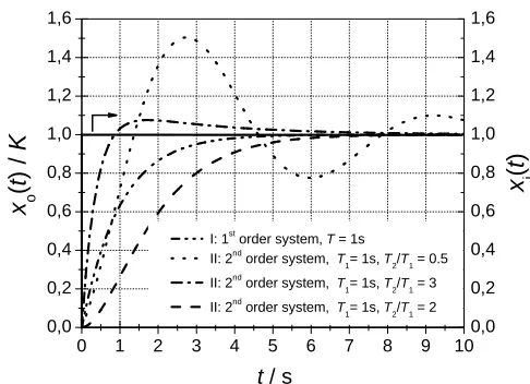
Figure 10.Normalized sensor output signals xo/K for the different
sensor types and different sensor parameters (interrupted lines) for a unit step input (solid line).
a defined dynamic response that cannot be modified. Typical step responses of sensor types I and II with different sensor parameters are exemplarily illustrated in Fig. 10.
4 General sensor model with compensation method
4.1 System model
Sensors using the compensation method exhibit a closed-loop feedback structure where the deflection is brought back to zero by a compensation force. This causes a force equi-librium and keeps the deflection of the sensor – occasionally with a small remnant control deviation – at zero. The de-flection can no longer be the measurement signal because it amounts more or less to zero. The sensor signal being pro-portional to the measurand is now the compensation force or an electrical quantity creating this compensation force. The resulting compensation circuit must at least contain the sen-sor itself, an amplifier, and the controller/actuator unit. Other components (e.g. D/A converter, filter) may be necessary, but do not alter the general system behavior and are thus ne-glected in this study. Because we act on the assumption of an electrical sensor output signal, amplification with a high-gain amplifier is assumed. For the sake of simplicity, we as-sume the amplifier, actuator, and controller to be much faster than the sensor itself. This would be particularly the case for, e.g. mechanical and chemical sensors. Hence, we can con-sider the actuator and the controller as one block placed in the feedback path. For other sensor types, where this sim-plifying assumption does not hold, the closed-loop sensor model with only one block in the feedback path is never-theless applicable. In this case, the dominant time constant of the feedback block is a combination of the time constants of the actuator and the controller parameters, respectively. The sensor with compensation is illustrated in Fig. 11. Note
X ’
iX
c
-Sensor
Controller
X
oG
s’(
s
)
V
G
c(
s
)
-
X
refX
iF
D
X
Figure 11.Closed-loop compensation circuit where the sensor out-put signal Xo is fed back to the sensor input via an amplifier and
a controller. F is a transfer element transforming an arbitrary input quantity in a quantity which can be actually compensated.
that the input signal X0i of the feedback structure is not nec-essarily the measuring quantity Xi. If a direct compensation of Xiis not possible, because the desired quantity cannot be generated by an existing device or the generation is too com-plicated, an equivalent quantity X0
i, which is correlated to Xi as X0
i =F·Xiand which is accessible for compensation must exist. This is a necessary requirement for the applicability of the compensation method to a certain sensor. The correlation between Xiand Xi0can be a simple factor (e.g. the gravity of Earth connecting mass and force in a balance) or rather com-plex (e.g. broadband lambda-probe or closed-loop hydrogel-based sensors (Schulz et al., 2011)), depending on the spe-cific sensor. In any case, the overall system behavior of the compensation circuit is independent of F. Therefore, to keep simplicity without loosing generality, we assume F=1 and thus, X0i=Xiand G0s=Gsfor all further considerations.
Initially, the input signal Xicauses the sensor output signal Xo. Xois amplified to V·Xo, the preset reference value Xrefis subtracted from it and fed back to the controller that gener-ates the compensation quantity Xc. Hence, Xccounteracts the sensor input signal. Assuming ideal compensation, the sensor input Xi−Xcis balanced during the whole measuring process in such a way that∆X and hence V·Xo−Xrefbecomes zero at the steady state. Hence, the sensor output Xoremains con-stant, independent of changes of the input signal. However, the “force” Xc, which is necessary to compensate changes of the input signal, depends on the input signal. Therefore, Xc is a measure of the input signal Xi and thus the output sig-nal of the “force”-compensated sensor. The resulting transfer function of the compensation circuit can then be written as
Gcomp(s)= Xc(s) Xi(s)
= V·Gs(s)·Gc(s) 1+V·Gs(s)·Gc(s)
= G(s)˜
1+G(s)˜ , (10)
with
˜
G(s)=V·Gs(s)·Gc(s) (11)
and expressed in a more general form as
Gcomp(s)=
Ncomp(s) Dcomp(s)
=cmsm+...+c1s+c0 dnsn+...+d1s+d0
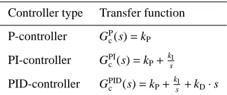
Table 3.Transfer functions of basic linear standard controller types (Datta et al., 2000).
Controller type Transfer function
P-controller GP c(s)=kP
PI-controller GPI
c(s)=kP+ksI
PID-controller GPID
c (s)=kP+ksI+kD·s
where both numerator Ncomp and denominator Dcomp are composed of polynomials. From Eq. (10) one can see that for Gcomp,0, the compensation quantity Xccan be used as a direct measure of the measuring quantity Xi. Because of the feedback loop, a transfer function in the form ˜G/(1+G) arises˜ (cp. Table 1), which exibits a completely different structure compared to the simple open-loop transfer function. More-over, the system properties can now be tuned and adjusted in certain limits via the amplifier gain and the parameters of Gc. Thus, Gcompcan be regarded as a variably tunable trans-fer function.
The controller is assumed to be a standard linear P-, PI-, or PID- controller, respectively. In principle, a specific con-troller could be designed for the task of compensation. How-ever, practically, the predominant majority of all control tasks are realized by standard controllers (Visioli, 2006). There-fore, we focus on those standard controllers. The transfer functions of the three controller types are listed in Table 3. Here, kPis the P-factor, kI the I-factor, and kDthe D-factor, with
kI= kP TI
and kD=kPTD, (13)
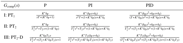
where TI and TD are the integral time and the differential time of the controller, respectively. We assume kP, kI, and kDto be constant. The application of the controller transfer functions Gc(s) from Table 3 and the sensor transfer func-tions Gs(s) from Table 2 to Eq. (10) leads to the closed-loop transfer functions of the three sensor types. The resulting transfer functions of the different sensor–controller combi-nations are listed in Table 4 where K∗=K·V. In the fol-lowing, K∗·k
P is termed as feedback factor. However, the most important requirement for a technical use of a closed-loop system is the system stability, i.e. a bounded input signal leads to a bounded output signal (BIBO-stability) (Shinners, 1998). Stability has to be guaranteed for all operating condi-tions. This necessitates the analysis of the closed-loop trans-fer functions to determine the parameter range in which the system is stable.
4.2 Stability requirements
Stability analysis is easily accessible in the frequency domain by analysis of the closed-loop transfer function Gcomp(s), as
stated in Eq. (12). This transfer function is asymptotically stable if and only if
– Gcompis proper, i.e. the degree m of the numerator Ncomp is smaller or equal to the degree n of the denominator Dcomp(m≤n, see Eq. 12), and
– if all poles of Gcompare placed in the complex left open
half-plane (LOH).
The first stability condition can be easily evaluated by a sim-ple look at the respective closed-loop transfer function (Ta-ble 4). The second stability condition can be verified by a stability criterion (e.g. Routh criterion (Shinners, 1998) as used within this work) applied to the denominator polyno-mial Dcomp(s). Here, the necessary condition is that all coeffi -cients dνof the denominator have the same sign (Stodola con-dition: Stodola, 1894; Hurwitz, 1895) (e.g. dm,..., d0>0). The sufficient condition results from the employed stability criterion and has to be evaluated subsequently. If the numer-ator degree amounts to n≤2, the Stodola condition is also sufficient. For that simplified case, no stability criterion has to be used in addition.
Table 4.Closed-loop transfer functions Gcomp(s) for all sensor-controller combinations considered; K∗=K·V.
Gcomp(s) P PI PID
I: PT1
K∗k
P
sT+(K∗k
P+1)
K∗(k
Ps+kI)
s2T+(1+K∗k
P)s+K∗kI
K∗(k
Ds2+kPs+kI)
(T+K∗k
D)s2+(1+K∗kP)s+K∗kI
II: PT2 K
∗
kP
T2
1s2+T2s+(1+K∗kP)
K∗(kPs+kI) T2
1s3+T2s2+(1+K∗kP)s+K∗kI
K∗(kDs2+kPs+kI) T2
1s3+(T2+K∗kD)s2+(1+K∗kP)s+K∗kI
III: PT2-D K
∗k
PT3s
T2
1s2+(T2+K∗kPT3)s+1
K∗T
3(kPs+kI)
T2
1s2+(T2+K∗kPT3)s+(1+K∗kIT3)
K∗T
3(kDs2+kPs+kI)
(T2
1+K∗kDT3)s2+(T2+K∗kPT3)s+(1+K∗kIT3)
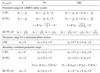
parameter range meeting both requirements is stated. As can be seen in Table 5, for the combination of a sensor with PT2 behavior together with a PI- or PID-controller, respectively, the degree of the denominator is of order three. Because of that, the Routh criterion derived from the Routh table has been used to get the sufficient stability condition. Stability analysis by utilization of the Routh criterion is explained in more detail in Appendix A. From these considerations it turns out that the range of controller parameters guarantee-ing stability depends on the sensor properties. Note that the second stability condition is even satisfied if certain parame-ters exhibit negative values. However, if one claims stability and minimum-phase behavior at the same time, the controller parameters do not depend on the sensor properties. The pa-rameters can be any positive value or even equal zero, except for the combination of a PT2 element with a PI- or a PID-controller. This enables a wide range of possible controller parameters for the adjustment of the desired system behav-ior for specific applications. Moreover, these findings do not show any contradiction towards the application of the com-pensation method in a technical measurement system. How-ever, from a practical point of view, the static feedback gain cannot be increased ad infinitum. Above a certain critical gain, a finite lag of the feedback path will lead to instabil-ities.
4.3 Steady state behavior
4.3.1 Static deviation from ideal compensation
The designated aim of the compensation method is ideal compensation of the sensor input Xi, such that V·Xo−Xref becomes zero at the steady state (s→0, t→ ∞ ). For the sake of simplicity, let us assume Xref=0. Then,
∆X=Xi−Xc=Xi−(V·Gs·Gc·∆X) (14) should be consequently as small as possible. From Eq. (14) we can set up a transfer function G∆between the compensa-tion deviacompensa-tion∆X and the input signal Xias
G∆:=G∆XX
i = ∆X(s)
Xi(s)
= 1
1+V·Gs·Gc
. (15)
Since Eq. (15) comprises the same denominator as the gen-eral transfer function in Eq. (10), we can act on the assump-tion that all poles of G∆ exhibit negative real part (for the
parameter range in Table 5), and that the transfer function is thus stable. In this case, one can apply the final value theorem of the Laplace transform, generally written as
lim
t→∞x(t)=lims→0[s
·X(s)]. (16)
Using Eq. (16), we can calculate the deviation ∆x(t→ ∞) from ideal compensation in the steady state for a step change of Xias
∆x(∞)=lim
t→∞∆x(t)=lims→0
s·G∆(s)·1
s
=lim
s→0G
∆(s). (17)
Example: PT1-type sensor with P-controller
For the simplest example of a PT1-type sensor in combina-tion with a P-controller, G∆is
G∆(s)= sT+1 sT+K∗k
P+1
, (18)
leading to
∆x(∞)=lim
s→0
sT+1
sT+K∗k
P+1
= 1
1+K∗k
P
. (19)
Table 5.Parameter range guaranteeing BIBO-stability and a minimum-phase system, and the resulting combined parameter range satisfying both requirements for all considered sensor-controller combinations.
Gcomp(s) P PI PID
Parameter range for a BIBO-stable system
I: PT1 kP>−K1∗ kP>−K1∗, kI>0 kP>−K1∗, kI>0, kD>−KT∗
II: PT2 kP>−K1∗ kP>−K1∗, kI>0 kP>−K1∗, kI>0, kD>−KT2∗
1+K∗
kP− T2
1K
∗k
I
T2 >0
a 1+K∗
kP− T2
1K
∗k
I
T2+K∗kD >0
a
III: PT2-D kP>− T2
K∗T
3 kP>−
T2
K∗T
3, kI>−
1 K∗T
3 kP>−
T2
K∗T
3, kI>−
1 K∗T
3, kD>−
T21 K∗T
3
Parameter range for a minimum-phase system
I-III: kP≥0 kP≥0, kI≥0 kP≥0b, kI≥0, kD≥0
Resulting combined parameter range
I: PT1 kP>0c kP≥0, kI>0 kP>0d, kI>0, kD≥0
II: PT2 kP>0 kP≥0, kI>0 kP>0, kI>0, kD≥0
T2(1+K∗kP)>T12K
∗
kIa (T2+K∗kD)(1+K∗kP)>T12K
∗
kIa
III: PT2-D kP>0 kP≥0, kI≥0 kP>0d, kI≥0, kD≥0
aThis criterion results from the application of the Routh criterion.
bExcept for k
D=0, this case is however not relevant due to the stability requirement.
cThe case k
P=0 is not relevant for sensor applications.
dk
P>0 instead of kP≥0 excludes the imaginary zero pair.
Table 6.Static deviation from ideal compensation for all considered sensor-controller combinations.
∆x(∞) P PI PID PT1 1+K1∗k
P 0 0
PT2 1+K1∗k
P 0 0
PT2-D N.A. K∗T1
2kI+1 1 K∗T
2kI+1
signal. However, a PI- or a PID-controller can be success-fully applied. The application of PI- or PID-controller to this sensor type leads to a static deviation that depends on the feedback factor, the integral time TIand the time constant T2. Thus, for a high feedback factor and a small integral time, the static deviation converges to zero.
4.3.2 Influence of static parameter variations
For a static analysis of the compensation circuit, we as-sume the closed-loop system to be in a steady state (Gstat
comp=
Gcomp(s→0)). So far, we have considered an ideal sensitivity K for the transfer function of the compensation circuit. How-ever, as described in the general sensor model in Sect. 3.1, the sensitivity is usually influenced by the interference quan-tity. Furthermore, compared to the open-loop sensor, the
am-plifier and the controller parameters can exhibit deviations from ideal behavior as well. Considering small static varia-tions, the impact of these deviations on the output signal Xc can be calculated by a first-order Taylor-series as
comp
s =
∆Xc Xc
= 1
Xc
∂Xc
∂K ·∆K+ ∂Xc
∂V ·∆V+ 3
X
i=1
∂Xc ∂ki
·∆ki
. (20)
Here, ki∈ {kP, kI, kD}and∆ki∈ {∆kP,∆kI,∆kD}are the con-troller parameters and their systematic deviations, respec-tively, depending on which controller type is used.
Example: PT1-type sensor with P-controller
For the simplest example of a PT1-type sensor in combina-tion with a P-controller,scompis
comp
s =
1+KVkP KVkP
Vk
P (1+KVkP)2
∆K+ KkP (1+KVkP)2
∆V
+ V K
(1+KVkP)2
∆kP
= 1
1+K∗k
P
∆K
K +
∆V V +
∆kP kP
. (21)
0 , 1 1 1 0 1 0 0 0 , 0
0 , 5 1 , 0 1 , 5 2 , 0
= 0 . 0 1 = 0 . 1 = 1
sc
o
m
p
/
sd
e
fl
K
*k
PP
P I , P I D
Figure 12.Ratio between systematic static deviations of the closed-loop sensor and the open-closed-loop sensor versus the feedback factor K∗
kPfor a PT1-type sensor in combination with all three controller
types.βindicates different deviation contributions from the feed-back elements compared to the deviation of the sensor itself.
summarized as a feedback deviation∆F B and can generally be described as a multiple (β) of the sensor deviation as
∆F B F B =
∆V
V +
∆kP kP =
β·∆K
K . (22)
Thus, Eq. (21) becomes
comp
s =
1+β 1+K∗k
P
∆K
K . (23)
The ratio between the relative systematic static deviation of the closed-loop compensation circuit and the open-loop sen-sor is
comp s defl
s
= 1+β
1+K∗k
P
. (24)
This ratio is illustrated in Fig. 12 as a function of the feed-back factor, and of β, indicating the deviation contribution of the feedback elements. Usually, the feedback elements should be designed such that systematic deviations are much smaller than the deviations of the sensor itself. As can be seen from Fig. 12, if the feedback deviations are just 1 % (β=0.01) of the sensor deviations, a unity feedback already minimizes the overall deviation to 50 % compared to an open-loop sensor. However, if the circuit comprises higher feedback deviations, the feedback factor can be systemati-cally increased to achieve a specified lower deviation of the output signal. If one wants to achieve a constant uncertainty, the required feedback factor linearly increases with β, as stated in Eq. (24).
The ratios between the deviations of the closed-loop con-figuration compared to the open-loop sensor for all sensor-controller combinations are listed in Table 7. From this table,
Table 7.Systematic static deviations of the closed-loop sensor for all sensor-controller combinations.
comp
s P PI PID
PT1 ∆K
K+∆VV+∆kPkP
1+K∗k
P 0 0
PT2 ∆K
K+∆VV+
∆kP kP
1+K∗k
P 0 0
PT2-D N.A. ∆K
K+∆VV+
∆kI kI
1+K∗k
PT3TI
∆K K+∆VV+
∆kI kI
1+K∗k
PT3TI
X
iX
c-
V
G
c(
s
)
-
X
refs+d
s K~(s)=K
D
X
Figure 13.Closed-loop compensation circuit where the quasi-static sensor part is characterized by a sensitivity ˜K, describing the dy-namics of the drift process by a drift model.
one can see that for PT1- and PT2-type sensors in combina-tion with a P-controller, the systematic deviacombina-tions depend on the deviation contributions of the single circuit elements and the feedback factor. However, by additional application of an I-part (PI- or PID-controller), the systematic deviations can be completely eliminated and no longer depend on the devi-ations of the circuit elements. For a PT2-D-sensor in combi-nation with a PI- or PID-controller, a similar behavior as dis-cussed for the P-controller before can be observed. Here, the overall deviation of the output signal cannot only be tuned by the static amplification V and the P-factor kP, but additionally by the integral time TI. The smaller the integral time is, the better is the resulting suppression of deviations.
Table 8.Closed-loop transfer function G∆compK,d considering a
time-dependent sensitivity ˜K instead of an ideal static sensitivity K by application of the drift model from Eq. (7) to the static sensor part (grey box in Fig. 13).
G∆compK,d(s)
P K∗kP(s+δ)
(1+K∗k
P)s+K∗kPδ
PI K∗kPs2+(K∗kI+K∗kPδ)s+K∗kIδ
(1+K∗k
P)s2+(K∗kI+K∗kPδ)s+K∗kIδ
PID K∗kDs3+(K∗kP+K∗kDδ)s2+(K∗kI+K∗kPδ)s+K∗kIδ
K∗k
Ds3+(1+K∗kP+K∗kDδ)s2+(K∗kI+K∗kPδ)s+K∗kIδ
transfer functions are exactly proper. The parameter range enabling a stable as well as a minimum-phase system is de-termined according to the criteria in Sect. 4.2 and listed in Table B1. From this table one can see that the system can be operated in a broad parameter range without jeopardizing the system stability. For the utilization of a P- or PI-controller, the controller parameters have to be simply positive to assure a stable minimum-phase system. For a PID-controller, the restrictions seem more complicated. However, if one simpli-fies the expression arising from the Routh table, one finds that again all of the stated requirements are met for posi-tive controller parameters (kP, kI, kD>0) independent of the drift-rate (see Sect. B1 in Appendix B). In this sense, stabil-ity directly involves a system without drift, because a system exhibiting drift is a priori unstable. This can be shown by calculating the steady state behavior of the output signal (xc) considering a unit step input according to Eq. (16) as
xc(∞)=lim
t→∞xc(t)=lims→0G
∆K
comp(s)=1 (25)
and is valid for all three controller types. One can see that the output signal of the closed-loop system is constant at the steady state for all three controller types, whereas the output signal of the open-loop sensor diverges to infinity (cp. Fig. 9). To enable a quantitative comparison of the quality of drift suppression for the three different controller types in depen-dence on the controller parameters, the use of a global per-formance index is reasonable. A perper-formance index, which is easy to handle and meaningful at the same time, is the In-tegral Square Error (ISE) (Newton et al., 1964) which can be written in the time domain as
J=
∞
Z
0
∆x2(t)dt. (26)
Here, ∆x(t) is the difference between the input step xi= 1(t) and the actual sensor output signal xc (cp. Fig. 13). This integral is a function of the controller parameters J= f (kP,kI,kD). The requirement for best drift suppression is that J is as small as possible (J=! min). For a quantitative eval-uation of this requirement and to get reasonable analytical
Table 9.Performance index from Eq. 27 for drift suppression for the three controller types
Performance index J
P 1
2K∗k
Pδ(1+K∗kP)
PI 1
2K∗k
Pδ(1+K∗kP)+2K∗kI(1+K∗kP)
PID 1
2K∗k
Pδ(1+K∗kP)+2K∗kI(1+K∗kP)+2K∗2kPkDδ2
equations for J, the transformation from the time to the fre-quency domain is reasonable. Since we already proved sys-tem stability for all three controller types, we can use Parse-val’s theorem (Newton et al., 1964) for the accomplishment of the transformation as
J=
∞
Z
0
∆x2(t)dt = 1 2π
+∞
Z
−∞
|∆X(s)|2ds
= 2π1
+∞
Z
−∞
∆X(s)∆X(−s)ds (27)
with
∆X(s) = 1
1+Ks+sδVGc
·1
s
= k0+k1s+...+kr−1sr−1 l0+l1s+...+lrsr
, lr , 0 (28)
according to the system structure in Fig. 13 for a unit step input. The explicit general solution of this integral up to r= 10 can be found in Newton et al. (1964). The insertion of the respective controller transfer function into Eq. (28) gives the compensation deviation ∆X(s), as stated in Table B2. The solution of the integral according to Eq. (27) and Newton et al. (1964), respectively, leads to the quality criteria J for the three controller types as given in Table 9 (cp. Sect. B2). From Table 9 it is obvious that the equation
∂J ∂ki =
0, with ki∈ {kP,kI,kD} (29)
cannot be explicitly satisfied. No local minimum in depen-dence of the controller parameters can be found because the first derivatives (∂J/∂kP,∂J/∂kI,∂J/∂kD) only converge to zero for infinitely large controller parameters (kP, kI, kD→
(a)
(b)
(c)
0,0 0,5 1,0 1,5 2,0 2,5 3,0 0,90
0,92 0,94 0,96 0,98 1,00 1,02
x c
(
t
)
t / s
K*
kP = 10, K*
kI = 100
K*
kP = 10, K *
kI = 500
K*kP = 10, K *
kI = 1*10 4
0 2 4 6 8 10 12 0,4
0,5 0,6 0,7 0,8 0,9 1,0
xc
(
t
)
t / s
K*
kP = 1
K*
kP = 10
K*kP = 50
0 2 4 6 8 10 12 0,90
0,92 0,94 0,96 0,98 1,00 1,02
K*
kP = 10, K*
kI = 100, K*
kD = 0.5 K*
kP = 10, K*
kI = 100, K*
kD = 10 K*
kP = 10, K*
kI = 100, K*
kD = 100
xc
(
t
)
t / s
k
Pk
Ik
Ik
D 0 10 2030 40 50 0
10 20 30 40 500 10 20 30 40
0 10 20
30 40 50
0 10 20 30 40 500 10 20 30 40
-3 x 10
J
PI-3 x 10
J
PID* K kP = 1
* K kP = 5
* K kP = 10
0,1 1 10 100
0 500 1000 1500 2000 2500 3000 3500 4000 4500
0 1 2 3 4 5
JP
K*k
P x 10-3
70 90
x 10-3
10 20 30 40 50
Figure 14.Step response of the closed-loop sensor for selected controller parameters (left) and ISE performance index as a function of the respective controller parameter (all other parameters are fixed) (right) for a (a) P-controller, (b) PI-controller, and (c) PID-controller. The light gray region indicates a tolerance band of±1 % of the steady state value. For all graphs a drift rate ofδ=1 s−1was considered. the system experiences an input step, it instantaneously
fol-lows this step to a certain extent until it is damped and con-verges to unity. The higher the respective controller param-eter is, the less damping can be observed. Furthermore, the steady state is reached even earlier. Here, reaching the steady state means that the sensor signal sets in into a tolerance band of±1 % of xc(t)=1 (gray region) and does not leave it anymore. This trend also reflects in the ISE performance indices in Fig. 14 (right). Here, generally J is minimized for increasing controller parameters. Moreover, with increasing controller complexity, J is additionally minimized. However, it can be seen that the P-part has the strongest influence on the quality of drift suppression. It is noteworthy that even a feed-back factor of K∗k
P=1 leads to a complete drift-suppression
to decaying oscillations within the tolerance band (Fig. 14c, left), which is not an aspired behavior. Thus, we can con-clude that the use of a P-controller with high feedback gain can satisfactorily fulfill the demand of drift suppression. A PI-controller is recommendable, if a faster accomplishment of the steady state is aspired, or if the feedback factor cannot be increased due to technical limitations. However, the use of a PID-controller is basically possible but would not be very convenient.
4.3.4 Non-linearities and hysteresis
Even if engineering in measurement science aims at a prefer-ably linear system behavior, almost all sensors show non-linearities to some extent in a certain output signal range. It is known that a non-linearity of a sensor in closed-loop operation is linearized to a certain extent due to the actual operation around a reference working point as
Xref−ε≤V·Xo≤Xref+ε, (30)
whereas ε is kept minimal due to the feedback structure. Hence, in general, a sensor operated by the compensa-tion method will show linearized input–output characteristics compared to the same sensor operated in deflection method. However, this may not be valid for all sensors operated by the compensation method or may just be valid for a lim-ited input signal range. Here, a nonlinear system descrip-tion can be used because a simple nonlinear model may pro-vide better approximations of the sensor behavior over an expanded range of operation than linear models. Despite the existence of a nonlinear sensor part, the application of lin-ear controllers can be possible. We assume that the sensor dynamics can be decomposed into a static or time-varying nonlinear function f and a linear dynamic part, which is described by transfer function. For this system description, two system models, i.e. the Wiener model and the Hammer-stein model, are widely used because of their simplicity and physical meaning. Both models can be used to approximate a wide range of nonlinear dynamic systems (Narendra and Gallman, 1966). The Hammerstein model applied to a non-linear sensor in closed-loop configuration is shown in Fig. 15. A Wiener model has the reverse system structure where the linear dynamic part is followed by the nonlinear part. Oc-casionally, combined models with Wiener-Hammerstein or Hammerstein-Wiener structure are also used. The system identification and assignment to one of the above models is an intensive research field, which has to be considered sep-arately and is beyond the scope of this work. However, also for nonlinear sensors in closed-loop configuration, stability has to be assured for all operating conditions. If an exist-ing sensor can be approximated by one of the above models, the stability of the closed-loop system can be achieved if the non-linearity is bounded by a Lipschitz condition or satisfies an appropriate sector condition. The basic idea is to deter-mine the controller parameters which are included in ˜Glins (s)
X
iD
X
X
clin
G
~
(
s
)
G
s linV
G
cf
(D
X,t
)
-Figure 15.Hammerstein model of a nonlinear sensor in closed-loop configuration. The model comprises a static nonlinear part f ahead of a linear dynamic subsystem ˜Glin
s . The linear subsystem
is composed of the linear time-invariant part of the sensor trans-fer function as well as the linear amplifier and controller transtrans-fer functions.
in such a way that a specific stability criterion is fulfilled without consideration of the nonlinear part. Various stability criteria do exist for this class of systems, e.g. circle criterion or Popov’s criterion (Slotine and Li, 1991; Khalil, 1992).
Sensors exhibiting hysteresis are also nonlinear systems and can thus be described by the models introduced above. However, phenomenologically, the output signal of the core sensor element Gs is kept at a quasi-static state around a reference working point due to the feedback structure (see Eq. 30). Since hysteresis mainly arises from dissipative ef-fects like inner friction inside the core sensor element or large amplitudes (e.g. plastic deformation of a spring element un-der load), these effects are greatly suppressed by the compen-sation method when assuming an actuator without hysteresis.
4.4 Dynamic system behavior 4.4.1 Response time
In general, the sensor response time of any sensor-type is determined by the poles of its transfer function. In the sim-plest case, only one pole, and thus only one time constant, exists. However, for higher-order transfer functions, several poles do exist. The pole that is located nearest to the imagi-nary axis in the LOH is dominant and determines the time to reach equilibrium. The condition for response time reduction is that the dominant pole of the closed-loop system is located in the LOH relative to the dominant pole of the open-loop sensor
<{scompp }<<{sdeflp } (31)
as schematically shown in Fig. 16. As apparent from Table 4, the denominator coefficients of all transfer functions depend on the controller parameters. This directly implies that in principle the pole locations can be explicitly set in certain limits by tuning the controller parameters.
Example: PT1-type sensor with P-controller
r
response time reduction
response time increase
stable system unstable system Im{s}
Re{s} comp
s
px
Figure 16.Representation of the complex Gauss plane exhibiting the real part r of the dominant pole sdefl
p of the open-loop sensor
and the LOH relative to this pole (gray region). The dominant pole scompp of the closed-loop sensor has to be located in this half plane to
enable a response time reduction according to Eq. (31). ,
time is the combination of a PT1-type sensor with a P-controller. If one rearranges the respective transfer function from Table 4, one gets
Gcomp(s)= K∗kP 1+K∗k
P
· 1
1+s1+KT∗k
P
= Kcomp 1+sTcomp
(32)
with
Tcomp= T 1+K∗k
P
. (33)
From Eq. (32) one can observe that the closed-loop system is also a first-order system, however with a modified time constant Tcomp. This time constant depends on the impressed time constant T of the open-loop sensor itself and inversely on the feedback factor. Thus, T is reduced to Tcomp by the factor (1/(K∗k
P)) and converges to zero for K∗kP→ ∞. The time-dependent sensor output signal for a unit step input of the open-loop PT1-type sensor as well as the closed-loop sen-sor comprising a P-controller are shown in Fig. 17a for dif-ferent feedback factors.
From Fig. 17a, one can observe the influence of different feedback factors on the sensor response time and on the static control deviation, as discussed in Sect. 4.3.1. It is notewor-thy that even a unity feedback leads to a minimization of the closed-loop response time of 50 %, which can be seen in Fig. 17b. Here, the normalized closed-loop time constant is illustrated as a function of the feedback factor. Fig. 17c schematically illustrates the effect of the feedback structure on the pole location of the closed-loop sensor.
For the combination of more complex controller and sen-sor types, the transfer functions also become more complex. Hence, for denominator polynomials of increasing order (two
or higher), the analytical determination of the poles becomes more demanding. At order two a case differentiation has to be made. For order three a general analytical solution is still possible but not trivial and may not lead to valuable practical conclusions. Therefore, to check the feasibility of a response time reduction and to verify the influence of the different con-troller types on the response time of the closed-loop system, we use a similar method as already used to proof system sta-bility. This method verifies which requirements have to be fulfilled, so that all poles of the closed-loop transfer function are placed in the LOH relative to the dominant pole of the respective open-loop transfer function. This directly implies a response time reduction. The steps required to accomplish this are:
– The determination of the dominant poles of the
open-loop transfer functions sdeflp and its real parts r=
<{sdeflp }.
– The redevelopment of the denominator polynomials
Dcomp(s) of the closed-loop transfer functions at point s=r into the new polynomial Dr
comp(s)=d0r+d
r
1(s−r)+
...+dr
n(s−r)nusing the Horner scheme.
– The evaluation of the coefficients dr
0 ... d
r
n by applica-tion of the Stodola condiapplica-tion and addiapplica-tional applicaapplica-tion of the Routh criterion (for n>2) to Dr
compto evaluate if all poles of the closed-loop transfer functions are placed left of s=r (cp. gray region in Fig. 16).
– The extraction of the controller parameters required to
meet these conditions.
Table 10.Dominant time constants (|1/r|) of the three different sensor types as well as the requirements (parameter range) for a response time reduction of the closed-loop sensor for all considered sensor-controller combinations.
Open-loop sensor Closed-loop sensor
Sensor Dominant P PI PID
type time constant
|1/r|
I: PT1 T kP>0 kP>K1∗, kP>K1∗+
2kD
T
kI> kP
T kI>
kP
T − kD
T2a
kD>−KT∗b
II: PT2
(1)ϕ≤2: 2T1
ϕ – – kP>
ϕ2−4
4K∗ +
ϕkD
T1
kI>ϕ(4K
∗k
P−ϕ2+4)
8K∗T
1 −
ϕ2k
D
4T2 1
kD>
ϕT1
2K∗
2K∗[k
IT13−kDT1(1+K∗kP)+ϕK∗k2D]
T1(ϕT1−2K∗kD) >0
c
(2)ϕ >2:
2T1 −ϕ+ √
ϕ2−4
kP>0 kP>
ϕ√ϕ2−4−ϕ2+4
2K∗ kP>
T1(ϕ
√
ϕ2−4−ϕ2+4)+K�