ReseaRch aRticle
C
ALIBRATION ANDV
ALIDATION OFI
MMEDIATEP
OST-F
IRES
ATELLITE-D
ERIVEDD
ATA TOT
HREES
EVERITYM
ETRICSJay D. Miller1* and Brad Quayle2
1 USDA Forest Service, Pacific Southwest Region, Fire and Aviation Management,
3237 Peacekeeper Way, Suite 101, McClellan, California 95652, USA
2 USDA Forest Service, Remote Sensing Applications Center,
2222 West 2300 South, Salt Lake City, Utah 84119, USA
*Corresponding author: Tel.: +1-916-640-1063; e-mail: [email protected]
ABSTRACT
Since 2007, the USDA Forest Ser-vice’s Remote Sensing Applications Center (RSAC) has been producing fire severity data within the first 30 to 45 days after wildfire containment (i.e., initial assessments [IA]), for wildfires that occur on USDA Forest Service managed lands, to support post-fire management actions. Satel-lite image-derived map products are produced using calibrations of the relativized differenced normalized burn ratio (RdNBR) to the Compos-ite Burn Index (CBI), percent change in tree basal area (BA), and percent change in canopy cover (CC). Cali-brations for extended assessments (EA) based upon one-year post-fire images have previously been pub-lished. Given that RdNBR is sensi-tive to ash cover, which declines with time since fire, RdNBR values that represent total mortality can be dif-ferent immediately post fire com-pared with one year post fire. There-fore, new calibrations are required for IAs. In this manuscript, we de-scribe how we modified the EA cali-brations to be used for IAs using an adjustment factor to account for
RESUMEN
changes in ash cover computed through regression of IA and EA Rd-NBR values. We evaluate whether the accuracy of IA and EA maps are significantly different using ground measurements of live and dead trees, and CBI taken one year post fire in 11 fires in the Sierra Nevada and northwestern California. We com-pare differences between error matri-ces using Z-tests of Kappa statistics and differences between mean plot values in mapped categories using Generalized Linear Models (GLM). We also investigate whether map ac-curacy is dependent upon plot dis-tance from boundaries delineating mapped categories. The IAs and EAs produced similarly accurate broad-scale estimates of tree mortali-ty. Between IAs and EAs of each se-verity metric, the Kappa statistics of error matrices were not significantly different (P > 0.674) nor were mean plot values within mapped categories (P > 0.077). Plots <30 m (one Land-sat pixel) distance from mapped polygon boundaries were less accu-rate than plots ≥30 m inside mapped polygons (P < 0.001). As land man-agers concentrate most post-fire management actions where tree mor-tality is high, it is desirable for map accuracy of severely burned areas to be high. Plots that were ≥30 m in-side polygons depicting ≥75 % or ≥90 % BA mortality were correctly classified (producer’s accuracy) >92.3 % of the time, regardless of IA or EA.
IA, usando un factor de ajuste que tiene en cuen-ta cambios en la cobertura de las cenizas, calcu-lado a través de una regresión de valores de IA y EA RdNBR. Evaluamos si la exactitud de los mapas de la IA y la EA son significativamente diferentes utilizando mediciones en terreno de árboles vivos y muertos, y el CBI tomado un año después del fuego en 11 incendios en Sierra Ne-vada y en el noroeste de California. Compara-mos las diferencias entre los errores matriciales con los Z-tests de las estadísticas de Kappa y las diferencias entre los valores medios de las par-celas en categorías mapeadas utilizando el Mo-delo Lineal Generalizado (GLM; generalizad li-near model). También investigamos si la exacti-tud de los mapas es dependiente de la distancia de la parcela hasta los límites marcados en las categorías mapeadas. Los IA y EA produjeron estimadores de mortalidad de árboles de exacti-tud similar y en una escala amplia. Entre los IA y EA de cada medida de severidad, las matrices de error según las estadísticas de Kappa no re-sultaron diferentes de forma significativa (P > 0.674), como tampoco los valores medios de las parcelas en las categorías mapeadas (P > 0.077). Las parcelas a <30 m (un píxel de Landsat) de distancia, desde los límites del polígono mapea-do fueron menos exactas que las parcelas a ≥30 m dentro de los polígonos mapeados (P < 0.001). Como los gestores del manejo de tierras concen-tran la mayor parte de las acciones de manejo post-fuego, en donde la mortalidad de los árbo-les es grande, es deseable que la exactitud de los mapas sea alta, especialmente en áreas severa-mente quemadas. Las parcelas que estaban a ≥30 m dentro de los polígonos representando una mortalidad del área basal (BA) de ≥75 % o ≥90 % fueron correctamente clasificadas (exacti-tud del productor) más del 92.3 % de las veces, independientemente del IA o EA.
Keywords: basal area, California, extended assessment, fire effects, initial assessment, Klamath, Landsat, RdNBR, Sierra Nevada
INTRODUCTION
Multispectral satellite data have become an important data source used by the US federal land management agencies for mapping wild-land fire effects, commonly called “severity” maps (Eidenshink et al. 2007, USDA 2007, Parsons et al. 2010). These data not only as-sist land managers in making post-fire man-agement decisions, but they can provide in-sights into basic fire ecology, serve as a broad-scale monitoring tool, and provide information on modern fire regimes (e.g., van Wagtendonk and Lutz 2007, Miller et al. 2009b, Dillon et al. 2011, Miller et al. 2012a, Miller et al. 2012b).
There are two closely linked issues that complicate interpreting fire severity maps. First, the degree of severity is based upon an interpretation of how much a site has been al-tered, which can vary depending upon vegeta-tion type and the expected amount of time it will take a site to recover to the pre-fire state (Lentile et al. 2006, NWCG 2014). For exam-ple, a fire that kills all aboveground compo-nents of a shrub system may not be considered high severity if the shrub system typically re-covers within a few years, as opposed to a co-nifer forest that could take many decades to recover. Second, severity assessments are of-ten reported in broad categories (i.e., low, moderate, and high) and are generally ambigu-ous with respect to what the categories mean in terms of quantitative fire effects (e.g., the amount of tree mortality or change in canopy cover [CC]) (Lentile et al. 2006). Therefore, there is a clear need to develop a linkage be-tween satellite-derived severity maps and actu-al fire effects on the ground. Hence, Miller et al. (2009a) described calibrations of one-year post-fire satellite data to tree mortality and change in CC for conifer forests.
In the 1990s, US land management agen-cies began using the normalized burn ratio (NBR) spectral index to derive severity maps because of the sensitivity of the Landsat bands
used in the index were most sensitive to changes in pre-fire to post-fire vegetation (White et al. 1996, Miller and Yool 2002, Key and Benson 2006b). The NBR is formulated like the normalized difference vegetation in-dex (NDVI) except the Landsat Thematic Mapper (TM) 2.08 µm to 2.35 µm mid-infra-red (MIR) band is used in place of the mid-infra-red band, as follows:
(1)
where NIR is the Landsat TM 0.76 µm to 0.90 µm near-infrared band (wavelengths for Land-sat 8 are slightly different, but the similar bands can be integrated accordingly). The NIR wavelengths are primarily sensitive to chlorophyll, while the MIR wavelengths used in the NBR are primarily sensitive to water content, ash cover, and soil mineral content (Kokaly et al. 2007). The NBR ranges be-tween −1 and 1 just like NDVI but, in com-mon practice, NBR is scaled by 1000 to trans-form to integer trans-format (Key and Benson 2006b).
Although first appearing in the formal lit-erature in Miller and Yool (2002), Key and Benson were the first to subtract a post-fire NBR from a pre-fire NBR for mapping fires in an absolute change detection methodology (a differenced NBR [dNBR]) so that barren areas unchanged by fire would not appear as high severity (Key and Benson 2006b). However, dNBR must be individually calibrated for each assessment of fire severity because of dispari-ties in vegetation types and density (Spanner et al. 1990, Miller and Yool 2002, Kokaly et al. 2007). Miller and Thode (2007) described a new spectral index, a relativized version of the differenced normalized burn ratio (RdN-BR) that they claimed allowed for calibrations to field-measured variables to be applied to fu-ture fires without further field validation. Miller and Thode (2007) modified dNBR by dividing by a function of the pre-fire NBR:
ܰܤܴ ൌ ൬ܰܫܴ െ ܯܫܴܰܫܴ ܯܫܴ൰
(2)
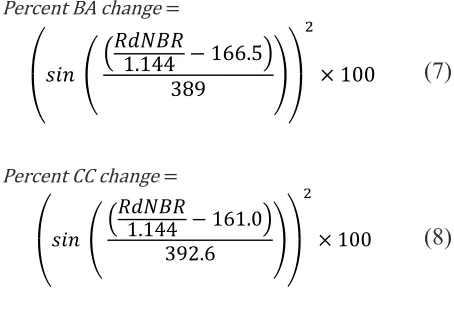
Miller and Thode (2007) published a cali-bration of RdNBR derived from one-year post-fire Landsat data (i.e., extended assessments [EA]) to the Composite Burn Index (CBI), a field based severity measure with values rang-ing from 0 to 3 (unchanged to high severity) that accounts for combined fire effects to sur-face fuels, understory, and upper canopy (Key and Benson 2006a). Consequently, it can be difficult to relate CBI values to a specific fire effect. Subsequently, Miller et al. (2009a) published calibrations of RdNBR EAs to two quantitative metrics: field-measured percent change in tree CC and basal area (BA). Esti-mates of all three metrics using RdNBR data are calculated as follows:
(3)
Percent BA change=
(4)
Percent CC change=
(5)
Miller et al. (2009a) also demonstrated that the calibrations produced fire severity classifications of similar accuracy in fires across a broad region of California that were not used in the original calibration process.
In 2006, the USDA Forest Service, Pacific Southwest Region, began developing methods to map severity to vegetation immediately post fire (i.e., initial assessments [IA] conducted within approximately 30 to 45 days of wildfire containment) to inform post-fire reforestation
planning for the national forests in California. Their methods were later adopted by the USDA Forest Service’s Remote Sensing Ap-plications Center (RSAC) under the Rapid As-sessment of VeGetation (RAVG) Condition program to extend coverage to all USDA For-est Service lands nationwide (USDA 2007). The RAVG program produces severity map products using the EA calibrations published in Miller et al. (2009a); however, there is one basic difference. Although NBR is primarily sensitive to changes in chlorophyll, the MIR wavelengths employed in the NBR are also sensitive to ash cover, which decreases over time due to wind and rain (Kokaly et al. 2007, Woods and Balfour 2008). As a result, RdN-BR values representing areas of complete mor-tality can differ between IAs and EAs. There-fore, new calibrations for IA post-fire images were necessary. However, there were not any immediate post-fire plot data available to de-rive new calibrations. The Pacific Southwest Region therefore modified the EA calibrations for CBI, and percent change in tree BA and CC to account for higher levels of ash cover that exist immediately post fire. In this paper, we first present the IA calibrations that were developed for California and were later adopt-ed by RSAC for the national RAVG program. Second, we use EA post-fire ground-based measurements used in Miller et al. (2009a) to assess the accuracy of IAs and compare them with EAs. Finally, considering that fires in forested landscapes can transition from surface to crown fire within 30 m, equal to the width of a Landsat pixel (Safford et al. 2012), we also compare the accuracy of BA ground mea-surements ˂30 m and ≥30 m distant from the inside boundary of mapped severity category polygons to determine how plot location and scale of the satellite data impacts classification accuracy.
��� � �0.3881 ��� �� ������� � 3��.0�421.7 �
����������������� � � ����� �������� � ������389 ��
�
� ���
������������������ � � ����� �������� � �6�.��392.6 �� �
� ���
����� � � �
� ����
���������� �����������1000 �� �
METHODS
Study Area
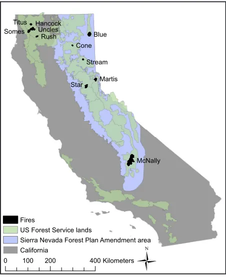
The fires used in this study were located within the region formed by the Sierra Nevada Forest Plan Amendment (SNFPA) planning area (USDA 2004) plus two national forests in northwestern California (Figure 1, Table 1).
The SNFPA planning area, which guides land and resource management on 50 000 km2
of national forest land on 11 US national for-ests, not only includes the Sierra Nevada and its foothills but also the Warner Mountains, Modoc Plateau, White Mountains, Inyo Moun-tains, and portions of the southern Cascades. Climate is mediterranean type, with warm, dry summers and cool, wet winters; nearly all pre-cipitation falls between October and April (Minnich 2007). Forest vegetation was di-verse, with different dominant species and high variation in density and vertical structure. The fires in this study were all located in mon-tane landscapes dominated by coniferous
for-est, with ponderosa pine (Pinus ponderosa Lawson & C. Lawson), Douglas-fir ( Pseudot-suga menziesii [Mirb.] Franco), and hard-woods (mostly Quercus spp.) dominant at low-er elevations; white fir (Abies concolor [Gord. & Glend.] Lindl. ex Hildebr.), incense cedar (Calocedrus decurrens [Torr.] Florin), sugar pine (Pinus lambertiana Douglas), ponderosa pine, and Douglas-fir at intermediate eleva-tions; and Jeffrey pine (Pinus jeffreyi Balf.), lodgepole pine (Pinus contorta Loudon), and red fir (A. magnifica A. Murray bis) at the higher elevations. The amount of understory vegetation was largely dependent on stand density, with open stands having more under-story vegetation.
Climate in northwestern California was also mediterranean, but somewhat moister on average than the SNFPA area, with higher spa-tial variability due to proximity to the Pacific Ocean and steep, complex topography (Skin-ner et al. 2006). While most of the dominant conifer species were shared with the Sierra Nevada and Cascade ranges, overall conifer diversity was higher with correspondingly greater vegetation diversity and complexity (Barbour et al. 2007). Midstory evergreen and deciduous hardwood trees were more abun-dant than in the Sierra Nevada (Sawyer and Thornburgh 1977).
Although total area burned per year on av-erage increased at the end of the twentieth cen-tury, much of the study area had not burned since before the beginning of the twentieth century (Miller et al. 2009b, Miller et al. 2012b, Mallek et al. 2013, Safford and Van de Water 2014).
Severity Data
The severity data for fires used in this study came from a database maintained by the USDA Forest Service’s Pacific Southwest Re-gion. The database contains fire severity data for most large wildfires since 1984 that have occurred at least partially on Forest Service Blue
Martis Star
Stream Cone
McNally Hancock
Rush Somes
Titus Uncles
Fires
US Forest Service lands
Sierra Nevada Forest Plan Amendment area California
Ü
0 100 200 400Kilometerslands in California. A majority of the RdNBR data used to produce the database was ac-quired from the Monitoring Trends in Burn Severity (MTBS; USDA-DOI 2005) and RAVG programs, but the database also con-tains many fires that were mapped by the Pa-cific Southwest Region. The MTBS protocols typically call for mapping fires in conifer for-ests using dNBR derived from a Landsat post-fire image acquired during the summer of the calendar year after fire containment (Key and Benson 2006b, Eidenshink et al. 2007). Al-though categorical severity maps produced by MTBS are produced from dNBR, MTBS also provides the non-calibrated RdNBR index data for each fire. The RAVG program produces severity maps (CBI, BA loss, and CC loss) within the first 30 to 45 days after wildfire containment. Conforming to best practices for a change detection methodology RAVG, MTBS and the Pacific Southwest Region chose pre- and post-fire images with the best possible matching anniversary dates to
mini-mize differences in sun angle, phenology, etc. (Singh 1989, Key and Benson 2006b). Before applying the calibrations to create categorical severity data, we applied a focal mean in a 3 × 3 pixel moving window to the RdNBR index data, which matched the 90-meter diameter of the field plots used to derive the calibrations, to reduce the number of single-pixel polygons in our database (Miller and Thode 2007). All severity data used in this study were derived from RdNBR, calculated from 30 m Landsat images, and calibrated to field measured CBI, percent change in BA, and percent change in CC.
Initial Assessment Calibrations
It is desirable to use ground reference data acquired near the same time as post-fire satel-lite data to train and assess the accuracy of de-rived classifications (Congalton and Green 1999, Jensen 2000). However, adequate post-fire plot data were not available when we
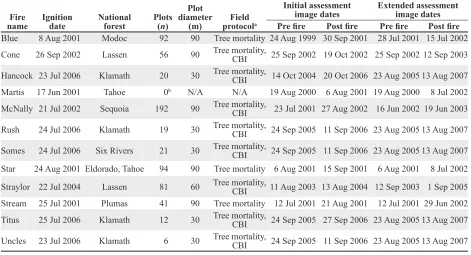
start-Fire
name Ignition date Nationalforest Plots(n) Plot diameter
(m) protocolField a
Initial assessment
image dates Extended assessment image dates
Pre fire Post fire Pre fire Post fire
Blue 8 Aug 2001 Modoc 92 90 Tree mortality 24 Aug 1999 30 Sep 2001 28 Jul 2001 15 Jul 2002
Cone 26 Sep 2002 Lassen 56 90 Tree mortality, CBI 25 Sep 2002 19 Oct 2002 25 Sep 2002 12 Sep 2003
Hancock 23 Jul 2006 Klamath 20 30 Tree mortality, CBI 14 Oct 2004 20 Oct 2006 23 Aug 2005 13 Aug 2007
Martis 17 Jun 2001 Tahoe 0b N/A N/A 19 Aug 2000 6 Aug 2001 19 Aug 2000 8 Jul 2002
McNally 21 Jul 2002 Sequoia 192 90 Tree mortality, CBI 23 Jul 2001 27 Aug 2002 16 Jun 2002 19 Jun 2003
Rush 24 Jul 2006 Klamath 19 30 Tree mortality, CBI 24 Sep 2005 11 Sep 2006 23 Aug 2005 13 Aug 2007
Somes 24 Jul 2006 Six Rivers 21 30 Tree mortality, CBI 24 Sep 2005 11 Sep 2006 23 Aug 2005 13 Aug 2007
Star 24 Aug 2001 Eldorado, Tahoe 94 90 Tree mortality 6 Aug 2001 15 Sep 2001 6 Aug 2001 8 Jul 2002
Straylor 22 Jul 2004 Lassen 81 60 Tree mortality, CBI 11 Aug 2003 13 Aug 2004 12 Sep 2003 1 Sep 2005
Stream 25 Jul 2001 Plumas 41 90 Tree mortality 12 Jul 2001 21 Aug 2001 12 Jul 2001 29 Jun 2002
Titus 25 Jul 2006 Klamath 12 30 Tree mortality, CBI 24 Sep 2005 27 Sep 2006 23 Aug 2005 13 Aug 2007
Uncles 23 Jul 2006 Klamath 6 30 Tree mortality, CBI 24 Sep 2005 11 Sep 2006 23 Aug 2005 13 Aug 2007
Table 1. Fires in this study and number of plots sampled one year post fire.
a CBI = Composite Burn Index; Tree mortality = species, live or dead, diameter at breast height, scorch height, crown base height,
and percent of crown volume scorched
ed to develop an IA methodology (circa 2006 to 2007). The only field data available in suf-ficient quantity were CBI and tree mortality data that had been collected one year post fire (Miller and Thode 2007, Miller et al. 2009a). Calibration of EA post-fire Landsat-derived RdNBR values to CBI had already been pub-lished, and a calibration to percent change in BA had been reported in a draft report (J. Mill-er and J. Fites, USDA Forest SMill-ervice, Nevada City, California, USA, unpublished report; Miller and Thode 2007).
As discussed earlier, in the pre- and post-fire change detection methodology we employ, wavelengths used in the RdNBR are primarily sensitive to changes in chlorophyll and ash cover (Key and Benson 2006b, Kokaly et al. 2007). However, additional tree mortality can occur for several years after a fire (Hood et al. 2010, van Mantgem et al. 2011). In addition, vegetation response (e.g., sprouting shrubs) in the first year post fire can result in higher chlo-rophyll levels in areas that experienced com-plete vegetation mortality (Crotteau et al. 2013). As we could not account for changes in chlorophyll due to delayed tree mortality or fire vegetative response using EA post-fire tree mortality data, we felt that the best ap-proach to developing calibrations for IAs was to adjust the EA calibrations to account only for differences in ash cover. To determine the average change in RdNBR due to changes in ash cover, we randomly selected areas with the following constraints: 1) they contain at least 1000 pixels representing unchanged condi-tions outside the fire perimeter and areas of complete tree mortality inside the perimeter, and 2) they were unaffected by post-fire man-agement actions, delayed tree mortality, or vegetative response (e.g., sprouting shrubs). The IA and EA RdNBR values were then gressed using ordinary least squares (OLS) re-gression. The IA RdNBR values in severely burned areas are primarily a function of ash cover and soil mineral content (Kokaly et al. 2007). We used EA RdNBR values as the
in-dependent variable as a proxy for soil mineral content in the regression model. Differences between pre- and post-fire images are always removed before computing RdNBR by sub-tracting the mean of unchanged areas from dNBR before computing RdNBR. The RdN-BR values for areas unaffected by fire or man-agement actions are therefore typically nor-mally distributed with a mean of zero as long as calendar dates of the pre- and post-fire im-ages are similar (Key and Benson 2006b, Mill-er and Thode 2007). Consequently, we did not include the intercept term in the OLS regres-sion model. The slopes of the regresregres-sions for a small representative set of fires were aver-aged and then incorporated as a linear scale factor into the EA post-fire calibrations. At the time (circa 2006 to 2007), Landsat images cost around $600 per scene and our funding for ac-quiring images was limited. In addition, through our experience in working with post-fire satellite imagery, we knew that there can be a high degree of variability between fires, and sometimes within fires, in the amount of decline in ash cover during the first year post fire. Therefore it would require only a small set of fires to obtain a rough estimate (within one SD) for the mean of ash cover decline, and a larger set of fires would not result in a more ro-bust estimate.
Accuracy Assessment
2001 to 2002, 60 m for 2004 fires, and 30 m for 2006 fires. Plots sampled in the SNFPA planning area were located at least 300 m apart on randomly placed transects. A stratified ran-dom procedure was used to generate potential plot locations for the 2006 fires in northwest California using a preliminary severity map. The CBI was not collected in fires that oc-curred during 2001, but was evaluated over the entire plot in subsequent years. Data collected to characterize fire effects on trees included status (live or dead), species, diameter at breast height (dbh), scorch height, crown base height (CBH), and percent of crown volume scorched. Tree data were collected for each tree in the 30 m diameter plots. The numbers of trees less than 10 cm in diameter were counted by species. In plots that were 60 m and 90 m in diameter, tree data were measured in four 10 m diameter subplots and tallied into 10-centimenter size classes. We estimated whether dead trees were killed by the fire or were already dead prior to the fire by presence or absence of dead needles as well as bark and wood consumption patterns. Live pre-fire trees are rarely consumed by fire (Pyne et al. 1996). But survival of pre-fire snags is depen-dent upon snag condition and fire intensity (Laudenslayer 1997, Skinner 2002). Pre- and post-fire BA was calculated from the diame-ters of trees thought to have been alive prior to the fire and alive after the fire, respectively. Pre- and post-fire CC was estimated using the Forest Vegetation Simulator (FVS; Dixon 2002). The FVS-derived estimates of individ-ual tree crown cover assume that trees are healthy and unaffected by fire or disease. We therefore adjusted FVS-computed CC using equations for modeling crown shape for north-ern California conifer species (Biging and Wensel 1990). (See Miller et al. [2009a] for more complete details on the CC calculations.) As USDA Forest Service vegetation classifica-tion standards require 10 % tree CC for an area to be classified as forested, we only used plots in this study for which FVS indicated ≥10% pre-fire tree CC (Brohman and Bryant 2005).
Analyses. We evaluated classification ac-curacy using error matrices detailing produc-er’s, usproduc-er’s, and overall accuracies and esti-mates of the Kappa statistic. Producer’s accu-racy (1 – omission error) is an evaluation of when a plot is not mapped in the correct cate-gory (i.e., a Type II error). User’s accuracy (1 – commission error) is an evaluation of when a plot is mapped in the wrong category (i.e., a Type I error). Kappa is a measure of the dif-ference between the actual agreement between reference data and classified data, and the chance agreement between the reference data and randomly classified data. Classifications can be statistically compared with Z-tests to determine whether classifications are signifi-cantly different (Congalton and Green 1999). We compared Kappa statistics of IAs and EAs, as well as Kappa statistics of plots that were ˂30 m and ≥30 m from mapped category boundaries of percent change in BA (Table 2).
for multiple comparisons (Kramer 1956). Fi-nally, we produced histograms of live tree BA in the highest BA mortality severity categories (≥75 % and ≥90 %) to illustrate how distance from the edge of mapped polygons (˂30 m, ≥30 m, and all plots) affects accuracy.
RESULTS
Initial Assessment Calibrations
The OLS regression slopes of initial to EA RdNBR values ranged between 1.069 and 1.193 (Table 3), resulting in a mean of 1.144 (SD = 0.053). The equations used to estimate CBI, percent change in BA, and percent change in CC from EA RdNBR values were modified as follows for IAs (Table 3: Miller et al. 2009a):
(6)
Percent BA change=
(7)
Percent CC change=
(8)
Accuracy Assessment
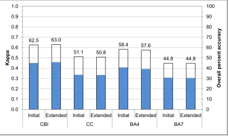
Initial vs. extended assessments. There were no significant differences between IA and EA Kappa statistics (Figure 2, all P ≥ 0.674). Comparing classifications of all plots, IA us-er’s and producus-er’s accuracies for the highest severity categories were greater than EAs, ex-cept for CBI (Table 4). However, there were no significant differences between mean plot
���� � �0.3881 ��� �� �������1.144 � 3��.0�421.7 �
������� �� ������ � �
���� � ������1.144 � 1��.��
389 �
� � �
� 1��
������� �� ������ � �
���� � ������1.144 � 161.��392.6 � � � �
� 1��
Composite burn index (CBI)
categories
Canopy cover (CC) change
categories Basal area change (BA4) categoriesBasal area change (BA7) categories CBI plots
(n) CC plots
(n) BA4a
plots (n)
BA4b plots (n)
BA7a plots (n)
BA7b plots (n)
Distance fr
om edge of severity category polygon
<30 m
0 % 0 % 51 39 56 42
>0 % and <10 % 54 64
>0 % and <25 % ≥10 % and <25 % 106 115 63 65
≥25 % and <50 % 75 80
≥25 % and <75 % ≥50 % and <75 % 115 119 67 66
≥75 % and <90 % 23 21
≥75 % ≥90 % 72 82 81 88
≥30 m
0 % 0 % 15 27 10 24
>0 % and <10 % 22 12
>0 % and <25 % ≥10 % and <25 % 40 31 7 5
≥25 % and <50 % 10 5
≥25 % and <75 % ≥50 % and <75 % 42 38 5 6
≥75 % and <90 % 3 5
≥75 % ≥90 % 193 183 158 151
All-plots distance
≥0 and <0 .1 0 % 0 % 0 % 9 72 66 66 66 66
>0 % and <10 % 76 76
≥0.1 and <1.25 >0 % and <25 % >0 % and <25 % ≥10 % and <25 % 98 137 146 146 70 70
≥25 % and <50 % 85 85
≥1.25 and <2.25 ≥25 % and <50 % ≥25 % and <75 % ≥50 % and <75 % 152 98 157 157 72 72
≥50 % and <75 % ≥75 % and <90 % 67 26 26
≥2.25 ≥75 % ≥75 % ≥90 % 141 260 265 265 239 239
Total 400a 634 634 634 634 634
Table 2. Number of plots by distance from edge of severity category polygon, severity category and as-sessment type. Lower case “a” and “b” denote initial and extended asas-sessments.
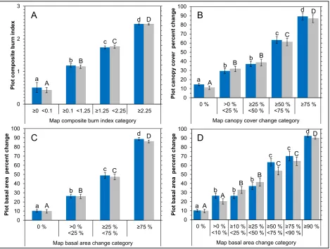
values of IA and EA classification categories (Figure 3, P = 0.077 for BA ≥10 % and <25 %, all other P ≥ 0.143).
User’s and producer’s accuracies were best for the highest severity categories, regardless
of severity metric (Table 4). Accuracies for lower severity categories of the percent change in BA and CC indicated that classification of individual plots was not much better than ran-dom. Accuracies of the low and middle CBI categories were a little better than the percent change in BA and CC.
Regardless of assessment, differences be-tween categories were significant for the four-category CBI and BA classifications (BA4; Figures 3A and 3C). When the number of categories increased, so did standard errors, resulting in differences between some adjacent categories not being significant (Figures 3B and 3D). Means of field-measured values in the lowest severity categories, regardless of assessment, were greater than what was ex-pected in the mapped categories (Figure 3). Means of field values for all other categories
62.5 63.0
51.1 50.8
58.4 57.6
44.8 44.8
0 10 20 30 40 50 60 70 80 90 100
0.0 0.1 0.2 0.3 0.4 0.5 0.6 0.7 0.8 0.9 1.0
Initial Extended Initial Extended Initial Extended Initial Extended
CBI CC BA4 BA7
Ov
era
ll
pe
rc
ent
a
cc
ura
cy
Kappa
Figure 2. Kappa statistic (blue bars) and overall classification accuracy (hollow bars with black outlines) for initial and extended assessment error matrices of Composite Burn Index (CBI), percent change in can-opy cover (CC), and basal area (BA) classifications. BA4 and BA7 refer to the four-category and sev-en-category basal area classifications. None of the comparisons of initial and extended assessment Kappa statistics are significantly different (all P > 0.674; Z ≥ 5.11).
Fire name Regression slope
Blue 1.069
Stream 1.156
Martis 1.193
Cone 1.157
Table 3. Fires used to estimate an average change in high severity RdNBR values between initial and extended assessments due to a decrease in ash cov-er. Regression slopes from ordinary least squares regression without an intercept in the model (all re-gressions R2
generally fell within the category ranges ex-cept for the seven-category BA classification (BA7).
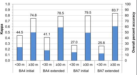
Distance from polygon boundary. Overall accuracy and Kappa values of plots ≥30 m from the mapped percent change in BA cate-gory boundary were higher when than when they were <30 m from the boundary (P <
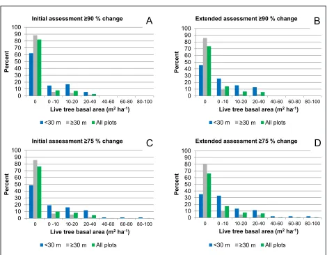
0.001; Figure 4). User’s and producer’s accu-racies were highest, ranging from 89.9 % to 100% for the highest (≥75 % or ≥90 %) severi-ty categories when plots were ≥30 m from the polygon boundary (Table 4). In contrast, us-er’s and producus-er’s accuracies ranged from 38.6% to 67.9 % when plots were <30 m from the polygon boundary. There were not any live trees in 81 % to 88 % of plots ≥30 m inside
Initial assessment Extended assessment
<30 m ≥30 m All plots <30 m ≥30 m All plots
CategoryUser’s (%) Producer’s (%) User’s (%) Producer’s (%) User’s (%) Producer’s (%) User’s (%) Producer’s (%) User’s (%) Producer’s (%) User’s (%) Producer’s (%)
Classification
Composite burn index
(CBI)
≥0
<0.1 36.4 44.4 27.3 66.7
≥0.1
<1.25 51.6 66.3 55.6 56.1
≥1.25
<2.25 58.9 50.0 58.3 55.3
≥2.25 78.4 74.5 79.3 75.9
Canopy cover
(CC)
0 % 28.9 38.9 40.2 48.6
>0 %
<25 % 33.7 40.9 39.0 43.8
≥25 %
<50 % 22.0 13.3 23.9 16.3
≥50 %
<75 % 22.2 17.9 18.8 19.4
≥75 % 83.3 82.7 77.0 76.2
Basal ar
ea
(BA4)
0 % 28.0 27.5 22.2 40.0 26.0 30.3 23.7 23.1 73.3 81.5 45.6 47.0
>0 %
<25 % 41.3 49.1 37.2 40.0 40.2 46.6 45.0 43.5 54.3 61.3 47.3 47.3
≥25 %
<75 % 46.0 40.0 50.0 21.4 46.6 35.0 36.4 36.1 34.6 23.7 36.1 33.1
≥75 % 60.3 56.9 92.1 96.4 84.1 85.7 50.0 53.7 89.9 92.3 77.2 80.4
Basal ar
ea (BA7)
0 % 28.0 25.0 22.2 60.0 26.0 30.3 23.7 21.4 73.3 91.7 45.6 47.0
>0 %
<10 % 16.3 24.1 45.5 22.7 19.8 23.7 33.3 34.4 46.2 50.0 35.4 36.8
≥10 %
<25 % 24.7 30.2 0.0 0.0 24.4 27.1 17.9 18.5 N/Aa 0.0 17.9 17.1
≥25 %
<50 % 21.3 17.3 25.0 10.0 21.5 16.5 20.8 20.0 N/Aa 0.0 20.8 18.8
≥50 %
<75 % 26.9 20.9 100.0 20.0 28.3 20.8 19.0 18.2 0.0 0.0 17.9 16.7
≥75 %
<90 % 8.7 17.4 N/Aa 0.0 8.7 15.4 11.1 23.8 N/Aa 0.0 11.1 19.2
≥90 % 67.9 44.4 92.4 100.0 86.6 81.2 48.6 38.6 90.7 96.7 77.9 75.3
Table 4. User’s and producer’s accuracies for initial assessments and extended assessments for all plots and for plots that were <30 m and ≥30 m from the edge of the severity category polygon in basal area (BA) classifications.
the highest severity polygons (EA ≥75 % BA change and IA ≥90 % BA change, respectively; Figure 5). In contrast, there were not any live trees in only 35 % to 62 % (EA ≥75 % BA change and IA ≥90 % BA change, respective-ly) of plots <30 m inside the highest severity polygons.
DISCUSSION
The modified EA calibrations that we used for IAs were based upon OLS regression of IA
and EA RdNBR values from four fires. We only used four fires in part because of the available data, but we also assumed that a small sample would produce a mean value that would be within one SD of the mean of a larg-er sample because of the high variation in ash cover decline between fires. In order to con-firm our assumption that a four-fire sample was adequate, we computed the mean of IA to EA regression slopes of all 12 fires (mean = 1.126, SD = 0.110, results not shown). The
0 10 20 30 40 50 60 70 80 90 100
0 % >0 %
<25 % <50 % ≥25 % <75 % ≥50 % ≥75 % Map canopy cover change category
Plot c anopy c ov er per ce nt c hange 0 10 20 30 40 50 60 70 80 90 100
0 % >0 %
<10 % ≥10 % <25 % ≥25 % <50 % ≥50 % <75 % ≥75 % <90 % ≥90 % Map basal area change category
Plot ba sa l a re a pe rc ent c hange 0 1 2 3
≥0 <0.1 ≥0.1 <1.25 ≥1.25 <2.25 ≥2.25
Map composite burn index category
Plot c omposi te burn inde x a A
b B
c C
d D
a A
b B
c C
d D
a A
a A
b B b B
c C
d D
b b
b
c c
d
A
B B
C C
D
A B
C D
0 10 20 30 40 50 60 70 80 90 100
0 % >0 %
<25 % ≥25 % <75 % ≥75 % Map basal area change category
Plot ba sa l a re a pe rc ent c hange
difference between the means from the four and twelve fire samples (0.018) was less than one SD of the four-fire sample (0.053), and a t-test of the difference between means was not significant (P = 0.38).
The IA calibrations derived using the four-fire sample adjustment factor produced classi-fications of similar accuracy to EA calibra-tions. Overall classification accuracies were similar and Kappa statistics were not signifi-cantly different between assessment types (Figure 2). Comparing category by category, there were not any significant differences in mean plot values between IAs and EAs (Fig-ure 3). Additionally, in a separate analysis, Safford et al. (2015) found no significant dif-ference in the percentage of high severity mapped by IAs and EAs within fires that oc-curred primarily in conifer forests on Forest Service managed lands in the Sierra Nevada (24.16 % vs. 23.99 %, IAs and EAs respective-ly; paired t-test P = 0.346, N = 53).
User’s and producer’s accuracies for low and middle severity categories were low for at least two reasons (Table 4). First, in most of the low and middle categories, there were more than twice as many plots <30 m from mapped category boundaries compared to the number of plots ≥30 m distant from boundar-ies (Table 2). It is therefore important to con-sider the registration accuracy of the satellite images and scale of the severity maps when using them for post-fire project planning. Plot location in relation to the boundary of the mapped severity polygons is important. Plots do not perfectly align with the 30 m satellite pixel, and as fire can transition from surface to crown within 30 m (Safford et al. 2012), fire effects can vary considerably within a pixel, resulting in lower accuracy for plots in the pix-el adjacent to the edge of the polygon. The middle severity categories often occur in nar-row bands around high severity patches. When the number of severity categories
in-44.5
74.8
41.1
78.5
27.0
79.5
25.8
83.7
0 10 20 30 40 50 60 70 80 90 100
0.0 0.1 0.2 0.3 0.4 0.5 0.6 0.7 0.8 0.9 1.0
<30 m ≥30 m <30 m ≥30 m <30 m ≥30 m <30 m ≥30 m
BA4 initial BA4 extended BA7 initial BA7 extended
Ov
er
al
l perc
ent ac
cura
cy
Kappa
0 10 20 30 40 50 60 70 80 90 100
0 0 -10 10-20 20-40 40-60 60-80 80-100
Pe
rc
ent
Live tree basal area (m2 ha-1)
Extended assessment ≥90 % change
<30 m ≥30 m All plots
B
0 10 20 30 40 50 60 70 80 90 100
0 0 -10 10-20 20-40 40-60 60-80 80-100
Per
cen
t
Live tree basal area (m2 ha-1)
Initial assessment ≥75 % change
<30 m ≥30 m All plots
C
0 10 20 30 40 50 60 70 80 90 100
0 0 -10 10-20 20-40 40-60 60-80 80-100
Per
cen
t
Live tree basal area (m2 ha-1)
Extended assessment ≥75 % change
<30 m ≥30 m All plots
D
0 10 20 30 40 50 60 70 80 90 100
0 0 -10 10-20 20-40 40-60 60-80 80-100
Pe
rc
ent
Live tree basal area (m2 ha-1)
Initial assessment ≥90 % change
<30 m ≥30 m All plots
A
Figure 5. Frequency of live tree basal area in field plots mapped at the highest severity in the percent bas-al area (BA) change classifications. Frequencies are for plots that were <30 m and ≥30 m inside the high-est severity polygon and all plots. Figures display field plots classified either ≥90 % or ≥75 % BA change by initial and extended assessments: A) initial assessment ≥90 % BA change, B) extended assessment ≥90 % BA change, C) initial assessment ≥75 % BA change, and D) extended assessment ≥75 % BA change.
creases (i.e., BA4 vs. BA7), those bands de-crease in width to only one to two pixels wide in many locations, leading to confusion be-tween severity categories (Figure 3). Consid-ering that pixels can be misregistered up to a pixel, it can also be impossible to identify the exact location of those moderate severity pix-els on the ground. Second, mean plot values in the lowest severity categories were greater than indicated by the mapped categories (Fig-ure 3). Kane et al. (2013) also detected tree mortality using LIDAR data in unchanged and low categories of maps calibrated to the CBI. All but two of the fires in our study occurred
(e.g., Landsat) under dense forest canopies (Stenback and Congalton 1990), leading to higher actual mortality measured in plots in the lower severity categories. Percent change in CC was based upon FVS calculations of pre- and post-fire live trees. The FVS esti-mates of CC were corrected for canopy over-lap, but FVS uses random tree placement (Crookston and Stage 1999, Miller et al. 2009a). Therefore, the percent changes in CC may not represent actual CC as seen from overhead by a satellite, thereby also leading to higher than expected CC change in the lowest severity categories. As a result, it may be more appropriate to combine the 0% category (BA or CC) with the next higher category (Kolden et al. 2012). When the 0 % and >0 % and <25 % change categories are combined, user’s and producer’s accuracies increase from ≥26.0 % to ≥62.4 % (results not shown).
Accuracies of the low and middle CBI cat-egories were a little better than the percent change in BA and CC metrics, perhaps be-cause CBI is a composite measurement repre-senting effects from surface fuels, understory vegetation, and the upper canopy (Key and Benson 2006a). However, the CBI protocol relies entirely upon ocular estimates, which can lead to considerable error (Korhonen et al. 2006).
Plot measured values we report for the lowest to mid-severity categories may not be representative of other vegetation types or of forests in other regions that are more or less productive, comprised of different species, or do not have a similar fire suppression history. However, it is likely that accuracies of the highest severity categories will be similar be-cause our methodology is dependent upon rel-ative change between pre- and post-fire imag-es (i.e., stand replacement regardlimag-ess of vege-tation type is always 100 % change).
There are two major factors that can con-tribute to differences between IAs and EAs. First, with the time delay between IA and EA image dates, any additional tree mortality or
resprouting or recovery of live vegetation can alter measured effects. Second, when fires are contained late in the calendar year, IA post-fire images may be acquired when the sun eleva-tion angle is low. Low sun angles, especially after the fall equinox at latitudes in our study area or farther north, can affect image quality in two ways: 1) the sun does not fully illumi-nate north-facing slopes in steep terrain, and 2) it can be difficult even on level terrain to see through tree canopies to the understory (Hol-ben and Justice 1980, Dymond and Qi 1997). When containment dates are late in the calen-dar year, a cloud-free post-fire image may not be available until the next spring due to cloud cover, thereby making an IA unfeasible. With-out immediate post-fire plot data re-measured one year post fire, we cannot assess whether delayed mortality was a factor in our classifi-cation accuracy. Consequently, we attempted to model only change in ash cover when modi-fying the EA calibrations. Some of our IA post-fire images were late in the calendar year (Table 1), so we therefore checked to see whether the IA RdNBR values for our plots were affected by steep north-facing slopes, and none appeared to be affected by topo-graphic shadows. Canopy shadowing may have been an issue as evidenced by lower IA accuracies of the lowest severity categories (Table 4), but there were not significant differ-ences between assessment types (Figure 3).
ACKNOWLEDGEMENTS
We wish to thank J. Baldwin for help with some of the statistics. We also wish to thank three anonymous reviewers whose comments greatly improved this manuscript. Finally, we would like to thank M. Landram, who had the original idea to begin the RAVG program, and T. Guay, who continues to do the operational day-to-day work in mapping IAs for RSAC.
LITERATURE CITED
Barbour, M.G., T. Keeler-Wolf, and A.A. Schoenherr, editors. 2007. Terrestrial vegetation of California. Third edition. University of California Press, Berkeley, USA. doi: 10.1525/ california/9780520249554.001.0001
Biging, G.S., and L.C. Wensel. 1990. Estimation of crown form for six conifer species of north-ern California. Canadian Journal of Forest Research 20: 1137−1142. doi: 10.1139/x90-151
Brohman, R., and L. Bryant, editors. 2005. Existing vegetation classification and mapping tech-nical guide. USDA Forest Service General Techtech-nical Report WO-GTR-67, Washington, D.C., USA.
Collins, B.M., R.G. Everett, and S.L. Stephens. 2011. Impacts of fire exclusion and recent man-aged fire on forest structure in old growth Sierra Nevada mixed-conifer forests. Ecosphere 2: art51. doi: 10.1890/ES11-00026.1
Congalton, R.G., and K. Green. 1999. Assessing the accuracy of remotely sensed data: princi-ples and practices. Lewis Publishers, Boca Raton, Florida, USA.
Crookston, N.L., and A.R. Stage. 1999. Percent canopy cover and stand structure statistics from the Forest Vegetation Simulator. USDA Forest Service General Technical Report RMRS-GTR-24, Rocky Mountain Research Station, Fort Collins, Colorado, USA.
Crotteau, J.S., J. Morgan Varner III, and M.W. Ritchie. 2013. Post-fire regeneration across a fire severity gradient in the southern Cascades. Forest Ecology and Management 287: 103−112.
doi: 10.1016/j.foreco.2012.09.022
Dillon, G.K., Z.A. Holden, P. Morgan, M.A. Crimmins, E.K. Heyerdahl, and C.H. Luce. 2011. Both topography and climate affected forest and woodland burn severity in two regions of the western US, 1984 to 2006. Ecosphere 2: art130. doi: 10.1890/ES11-00271.1
Dixon, G.E. 2002. Essential FVS: a user’s guide to the Forest Vegetation Simulator. USDA For-est Service, ForFor-est Management Service Center, Fort Collins, Colorado, USA.
Dymond, J.R., and J.G. Qi. 1997. Reflection of visible light from a dense vegetation cano-py—a physical model. Agricultural and Forest Meteorology 86: 143−155. doi: 10.1016/ S0168-1923(97)00028-2
from the boundary in the highest severity cate-gory had no live trees (Figure 5). As accuracy of IAs and EAs is similar, both appear to be adequate for producing broad-scale estimates and in identifying locations of complete tree mortality.
Currently, the calibrations presented in this manuscript are being utilized by the RAVG program for all initial post-fire assessments
Eidenshink, J., B. Schwind, K. Brewer, Z.-L. Zhu, B. Quayle, and S. Howard. 2007. A project for monitoring trends in burn severity. Fire Ecology 3(1): 3−21. doi: 10.4996/fireecology.0301003
Holben, B.N., and C.O. Justice. 1980. The topographic effect on spectral response from na-dir-pointing sensors. Photogrammetric Engineering and Remote Sensing 46: 1191−1200. Hood, S.M., S.L. Smith, and D.R. Cluck. 2010. Predicting mortality for five California
coni-fers following wildfire. Forest Ecology and Management 260: 750−762. doi: 10.1016/j. foreco.2010.05.033
Jensen, J.R. 2000. Remote sensing of the environment: an earth resource perspective. Prentice Hall, Upper Saddle River, New Jersey, USA.
Kane, V.R., J.A. Lutz, S.L. Roberts, D.F. Smith, R.J. McGaughey, N.A. Povak, and M.L. Brooks. 2013. Landscape-scale effects of fire severity on mixed-conifer and red fir forest structure in Yosemite National Park. Forest Ecology and Management 287: 17−31. doi: 10.1016/j.foreco.2012.08.044
Key, C.H., and N.C. Benson. 2006a. Landscape assessment: ground measure of severity, the Composite Burn Index. Pages LA8−LA15 in: D.C. Lutes, editor. FIREMON: Fire Effects Monitoring and Inventory System. USDA Forest Service Technical Report RMRS-GTR-164-CD, Rocky Mountain Research Station, Fort Collins, Colorado, USA.
Key, C.H., and N.C. Benson. 2006b. Landscape assessment: remote sensing of severity, the Nor-malized Burn Ratio. Pages LA25−LA41 in: D.C. Lutes, editor. FIREMON: Fire Effects Monitoring and Inventory System. USDA Forest Service Technical Report RMRS-GTR-164-CD, Rocky Mountain Research Station, Fort Collins, Colorado, USA.
Kokaly, R.F., B.W. Rockwell, S.L. Hiare, and T.V.V. King. 2007. Characterization of post-fire surface cover, soils, and burn severity at the Cerro Grande Fire, New Mexico, using hyper-spectral and multihyper-spectral remote sensing. Remote Sensing of Environment 106: 305−325.
doi: 10.1016/j.rse.2006.08.006
Kolden, C.A., J.A. Lutz, C.H. Key, J.T. Kane, and J.W. van Wagtendonk. 2012. Mapped versus actual burned area within wildfire perimeters: characterizing the unburned. Forest Ecology and Management 286: 38−47. doi: 10.1016/j.foreco.2012.08.020
Korhonen, L., K.T. Korhonen, M. Rautiainen, and P. Stenberg. 2006. Estimation of forest cano-py cover: a comparison of field measurement techniques. Silva Fennica 40: 577−588. doi: 10.14214/sf.315
Kramer, C.Y. 1956. Extension of multiple range tests to group means with unequal number of replications. Biometrics 12: 307−310. doi: 10.2307/3001469
Laudenslayer, W.F. 1997. Effects of prescribed fire on live trees and snags in eastside pine for-ests in California. Pages 256−262 in: M. Morales, and T. Morales, editors. Proceedings of the symposium: fire in California ecosystems: integrating ecology, prevention and manage-ment. The Association for Fire Ecology Miscellaneous Publication 1.
Lentile, L.B., Z.A. Holden, A.M.S. Smith, M.J. Falkowski, A.T. Hudak, P. Morgan, S.A. Lewis, P.E. Gessler, and N.C. Benson. 2006. Remote sensing techniques to assess active fire charac-teristics and post-fire effects. International Journal of Wildland Fire 15: 319–345. doi: 10.1071/WF05097
Leonzo, C.M., and C.R. Keyes. 2010. Fire-excluded relict forests in the southeastern Klamath Mountains, California, USA. Fire Ecology 6(3): 62−76. doi: 10.4996/fireecology.0603062
Miller, J.D., B.M. Collins, J.A. Lutz, S.L. Stephens, J.W. van Wagtendonk, and D.A. Yasuda. 2012a. Differences in wildfires among ecoregions and land management agencies in the Sier-ra Nevada region, California, USA. Ecosphere 3: art80. doi: 10.1890/ES12-00158.1
Miller, J.D., E.E. Knapp, C.H. Key, C.N. Skinner, C.J. Isbell, R.M. Creasy, and J.W. Sherlock. 2009a. Calibration and validation of the relative differenced Normalized Burn Ratio (RdN-BR) to three measures of fire severity in the Sierra Nevada and Klamath Mountains, Califor-nia, USA. Remote Sensing of Environment 113: 645−656. doi: 10.1016/j.rse.2008.11.009
Miller, J.D., H.D. Safford, M.A. Crimmins, and A.E. Thode. 2009b. Quantitative evidence for increasing forest fire severity in the Sierra Nevada and southern Cascade Mountains, Califor-nia and Nevada, USA. Ecosystems 12: 16−32. doi: 10.1007/s10021-008-9201-9
Miller, J.D., C.N. Skinner, H.D. Safford, E.E. Knapp, and C.M. Ramirez. 2012b. Trends and causes of severity, size and number of fires in northwestern California, USA. Ecological Ap-plications 22: 184−203. doi: 10.1890/10-2108.1
Miller, J.D., and A.E. Thode. 2007. Quantifying burn severity in a heterogeneous landscape with a relative version of the delta Normalized Burn Ratio (dNBR). Remote Sensing of Environ-ment 109: 66−80. doi: 10.1016/j.rse.2006.12.006
Miller, J.D., and S.R. Yool. 2002. Mapping forest post-fire canopy consumption in several over-story types using multi-temporal Landsat TM and ETM data. Remote Sensing of Environ-ment 82: 481−496. doi: 10.1016/S0034-4257(02)00071-8
Minnich, R.A. 2007. Climate, paleoclimate, and paleovegetation. Pages 43−70 in: M.G. Barbo-ur, T. Keeler-Wolf, and A.A. Schoenherr, editors. Terrestrial vegetation of California. Uni-versity of California Press, Berkeley, USA.
NWCG [National Wildfire Coordinating Group]. 2014. PMS 205 glossary of wildland fire ter-minology. <http://www.nwcg.gov/pms/pubs/glossary/index.htm>. Accessed 1 October 2014. Nelder, J.A., and R.W.M. Wedderburn. 1972. Generalized linear models. Journal of the Royal
Statistical Society. Series A (General) 135: 370−384. doi: 10.2307/2344614
Parsons, A., P.R. Robichaud, S.A. Lewis, C. Napper, and J.T. Clark. 2010. Field guide for map-ping post-fire soil burn severity. USDA Forest Service General Technical Report RMRS-GTR-243, Rocky Mountain Research Station, Fort Collins, Colorado, USA.
Pyne, S.J., P.L. Andrews, and R.D. Laven. 1996. Introduction to wildland fire. Second edition. John Wiley & Sons, New York, New York, USA.
Safford, H.D., J.D. Miller, and B.M. Collins. In press. Differences in land ownership, fire man-agement objectives, and source data matter: a reply to Hanson and Odion (2014). Internation-al JournInternation-al of Wildland Fire. doi: 10.1071/wf14013
Safford, H.D., J.T. Stevens, K. Merriam, M.D. Meyer, and A.M. Latimer. 2012. Fuel treatment effectiveness in California yellow pine and mixed conifer forests. Forest Ecology and Man-agement 274: 17−28. doi: 10.1016/j.foreco.2012.02.013
Safford, H.D., and K. Van de Water. 2014. Using fire return interval departure (FRID) analysis to map spatial and temporal changes in fire frequency on national forest lands in California. USDA Forest Service Research Paper PSW-RP-266, Pacific Southwest Research Station, Al-bany, California, USA.
Sawyer, J.O., and D.A. Thornburgh. 1977. Montane and subalpine vegetation of the Klamath Mountains. Pages 699−732 in: M.G. Barbour and J. Major, editors. Terrestrial vegetation of California. John Wiley and Sons, New York, New York, USA.
Singh, A. 1989. Digital change detection techniques using remotely-sensed data. International Journal of Remote Sensing 10: 989−1003. doi: 10.1080/01431168908903939
Skinner, C.N. 2002. Influence of fire on the dynamics of dead woody material in forests of Cali-fornia and southwestern Oregon. Pages 445−454 in: W. F. Laudenslayer Jr., P.J. Shea, B.E. Valentine, C.P. Weatherspoon, and T.E. Lisle, editors. Proceedings of the symposium on the ecology and management of dead wood in western forests. USDA Forest Service General Technical Report PSW-GTR-181, Pacific Southwest Research Station, Albany, California, USA.
Skinner, C.N., A.H. Taylor, and J.K. Agee. 2006. Klamath Mountains bioregion. Pages 170−194 in: N.G. Sugihara, J.W. Van Wagtendonk, J.A. Fites-Kaufman, K.E. Shaffer, and A.E. Thode, editors. Fire in California ecosystems. University of California, Berkeley, USA.
Spanner, M.A., L.L. Pierce, D.L. Peterson, and S.W. Running. 1990. Remote sensing of temper-ate coniferous forest leaf area index: the influence of canopy closure, understory vegetation and background reflectance. International Journal of Remote Sensing 11: 95−111. doi: 10.1080/01431169008955002
Stenback, J.M., and R.G. Congalton. 1990. Using Thematic Mapper imagery to examine forest understory. Photogrammetric Engineering and Remote Sensing 56: 1285−1290.
Taylor, A.H., and C.N. Skinner. 2003. Spatial patterns and controls on historical fire regimes and forest structure in the Klamath Mountains. Ecological Applications 13: 704−719. doi: 10.1890/1051-0761(2003)013[0704:SPACOH]2.0.CO;2
USDA [US Department of Agriculture]. 2004. Sierra Nevada forest plan amendment final sup-plemental environmental impact statement. USDA Forest Service Report R5-MB-046, Pacif-ic Southwest Region, Vallejo, California, USA.
USDA [US Department of Agriculture]. 2007. Rapid Assessment of Vegetation Condition after Wildfire (RAVG). <http://www.fs.fed.us/postfirevegcondition/index.shtml>. Accessed 1 Oc-tober 2014.
USDA-DOI [US Department of Agriculture-Departmet of the Interior]. 2005. Monitoring Trends in Burn Severity (MTBS) Project. <http://www.mtbs.gov>. Accessed 1 October 2014.
van Mantgem, P.J., N.L. Stephenson, E. Knapp, J. Battles, and J.E. Keeley. 2011. Long-term ef-fects of prescribed fire on mixed conifer forest structure in the Sierra Nevada, California. Forest Ecology and Management 261: 989−994. doi: 10.1016/j.foreco.2010.12.013
van Wagtendonk, J.W., and J.A. Lutz. 2007. Fire regime attributes of wildland fires in Yosemite National Park, USA. Fire Ecology 3(2): 34−52. doi: 10.4996/fireecology.0302034
Vankat, J.L., and J. Major. 1978. Vegetation changes in Sequoia National Park, California. Jour-nal of Biogeography 5: 377−402. doi: 10.2307/3038030
White, J.D., K.C. Ryan, C.C. Key, and S.W. Running. 1996. Remote sensing of forest fire sever-ity and vegetation recovery. International Journal of Wildland Fire 6: 125−136. doi: 10.1071/ WF9960125