Università degli Studi di Bologna
DEIS
Biometric System Laboratory
Pattern Recognition by Hierarchical Temporal Memory
Davide Maltoni
[email protected]
April 13, 2011
1
Pattern Recognition by Hierarchical Temporal Memory
Davide Maltoni,DEIS - University of Bologna (Italy)
Abstract—Hierarchical Temporal Memory (HTM) is still largely unknown by the pattern recognition community and only a few
studies have been published in the scientific literature. This paper reviews HTM architecture and related learning algorithms by using
formal notation and pseudocode description. Novel approaches are then proposed to encode coincidence-group membership (fuzzy
grouping) and to derive temporal groups (maxstab temporal clustering). Systematic experiments on three line-drawing datasets have
been carried out to better understand HTM peculiarities and to extensively compare it against other well-know pattern recognition
approaches. Our results prove the effectiveness of the new algorithms introduced and that HTM, even if still in its infancy, compares
favorably with other existing technologies.
IERARCHICAL temporal memory (HTM) is a biologically-inspired computational framework recently proposed by Hawkins and George [1-3] as a first practical implementation of the memory-prediction theory of brain function presented by Hawkins in [4]. A private company, called Numenta1 [5], was setup to develop HTM technology and to make available to researches and practitioners a complete development platform. A number of technical reports and presentations are available in Numenta website [5] to describe HTM technology, application and results, but at today few independent studies [6-12] have been published to validate this computational framework and to frame it into the state-of-the-art.
HTM substantially differs from traditional neural network implementations (e.g., a multilayer perceptron) and can be conveniently framed into Deep Architectures [13][14]. In particular, Ranzato et al. [15] introduced the term Multi-stage Hubel-Wiesel Architectures (MHWA) to denote a specific subfamily of Deep Architectures. An MHWA is organized in alternating layers of feature detectors (reminiscent of Hubel and Wiesel’s simple cells) and local pooling/subsampling of features (reminiscent of Hubel and Wiesel’s complex cells); a final layer trained in supervised mode performs the classification. Neocognitron [16], Convolutional Networks [17][18], HMAX and its evolutions [19][20] are the best known implementations of MHWA. In analogy with MHWA, HTM alternates feature detection and feature pooling; however, in HTM feature pooling heavily relies on the temporal analysis of pattern sequences while in Neocognitron is hardwired and in Convolutional Network and HMAX is performed through simple spatial operators such as max or average. The temporal analysis and the modeling as a Bayesian Network make HTM similar in some aspects to Hierarchical [21] or Layered [22] versions of Hidden Markov Models (HMM); however, while HMM attempts to model the intrinsic temporal structure of input patterns2, HTM exploits time continuity (mainly during learning) for unsupervised derivation of invariant representations, independently of the static or dynamic nature of the input patterns.
1 the author of this paper has no business relationships with Numenta or with its founders, and has no commercial interest in promoting HTM technology.
2
in fact, the most successful HMM applications are in domains where patterns have an intrinsic temporal structure (e.g., speech recognition) or a spatial structure
2 As pointed out by Hawkins and George "... many of these ideas existed before HTMs and have been part of other models. The power of HTM comes from a unique synthesis of these ideas". In our opinion, HTM is the result of brilliant intuitions and clever engineering, and although HTM is still in its infancy, in the future it could help dealing with invariance which is the holy grail problem of pattern recognition and computer vision. Why HTM should overcome existing techniques in tackling invariance? There are some important properties that can be exploited to this purpose:
The use of time as supervisor. A key problem in visual pattern recognition is that minor intra-class variations of a
pattern can result in a substantially different spatial representation (e.g., in term of pixel intensities). Huge efforts have been done to develop variation-tolerant metrics (e.g., tangent distance [23]) or invariant feature extraction techniques (e.g., SIFT [24]), but to date, successful results have been achieved only for specific problems. HTM exploits time continuity to claim that two representations, even if spatially dissimilar, originate from the same object if they come close in time. This concept, which constitutes the basis of Slow Feature Analysis [25], is simple but extremely powerful because it is applicable to whatever form of invariance (i.e., geometry, pose, lighting). It also enables unsupervised learning: labels are provided by the time.
Hierarchical organization. This is a largely used computation paradigm to put in practice the maxim "divide et
impera". Recently a number of studies provided theoretical support to the advantages of hierarchical systems in learning invariant representations [13][26]. As the human brain HTM uses a hierarchy of levels to decompose object recognition complexity: at low levels the network learns basic features which are used as building blocks at higher levels to form representations of increasing complexity. Building blocks are also crucial for efficient coding and generalization since through their combination HTM can encode new objects never seen before. Top down and bottom-up information flow. In MHWA information typically flows one-way from lowers levels to
upper levels. In the human cortex, both feed-forward and feed-back messages are continuously exchanged between different regions; although the precise role of feed-back messages is still very debated, neuroscientists agrees on their fundamental support in the perception of non-trivial patterns [4][27]. Memory-prediction theory postulates that feed-back messages from higher levels carry contextual information that can bias the behavior of lower levels. This is crucial to deal with uncertainty: if a node of a given level has to process an ambiguous pattern (e.g., a noisy version of an already encountered pattern) its decision could be better taken in presence of hints from upper levels, whose nodes are probably aware of the context the network is operating in (e.g., if one step back in time we were recognizing a car, probably we are still processing a traffic scene).
Bayesian probabilistic formulation. Probabilistic decisions are often better than binary choices when dealing with
3 Although HTM can be used in a variety of contexts, in this paper we focus only on visual recognition applications (i.e., inputs are 2D images). We also ignore biological aspects of HTM theory: an excellent description of HTM biological underpinning is reported in [3] where its implementation in terms of biological circuits is presented. When we started working with HTM we initially used the Numenta development platform, called Nupic [5] (most of the components are freely available to research organizations), but soon we decided to implement a new version from scratch: this is to have more flexibility and full control over the entire training/inference stages. Examples and experimental results reported throughout this paper have been obtained with our own HTM implementation.
The main contributions of this work are:
an extensive description of HTM architecture (Sections 1, 2 and 3) and learning algorithms (Section 4) with
consistent notation and pseudocode description;
the introduction of novel approaches (Section 5) to encode coincidence-group membership more robustly (Fuzzy
grouping) and to derive more stable temporal groups (MaxStab temporal clustering);
the implementation of fast learning procedures, based on temporary data-buffering, to speed-up the training stage
(Section 5.1.3);
an extensive experimentation on three line-drawing datasets (Section 6) aimed at: (i) finding out optimal HTM
architecture and parameters; (ii) assessing the effectiveness of Fuzzy grouping and MaxStab temporal clustering; (iii) comparing HTM with other existing approaches.
further experiments to understand (and quantify) the efficacy of HTM mechanisms such as overlapped
architectures (Section 6.2.3) and saccading (Section 6.2.5).
In Section 7 we draw some conclusions and summarize the huge amount of work we believe it is worth undertaking to overcome current HTM limitations and, hopefully, move some steps forward in solving challenging pattern recognition problems.
1.
OVERALL HTM STRUCTURE
An HTM is a tree-like network composed of (≥ 2) levels numbered from 0 to (see Fig. 1). is
the input level; is the output level; are called intermediate levels (if = 2 the
network has no intermediate levels). Each level is composed of nodes . Nodes in input, intermediate and output levels are called input, intermediate and output nodes, respectively. To make notation lighter,
a generic node can be denoted as and a generic node at level can be denoted as . When an HTM is used for visual pattern classification, typically:
input nodes are in 1:1 relationship with image pixels;
nodes in each level are arranged in a rectangular grid (i.e., retinotopic mapping of the input);
4 Fig. 1. A four-level HTM designed to work with 16x16 pixel images. Level 0 has 16x16 input nodes, each associated to a single pixel. Each level 1 node has 16 child nodes (arranged in a 4×4 region) and a receptive field of 16 pixels. Each level 2 node has 4 child nodes (2×2 region) and a receptive field of 64 pixels. Finally, the single output node at level 3 has 4 child nodes (2×2 region) and a receptive field of 256 pixels. In the figure only the downward connections of one node per level are shown.
levels are sequentially interconnected through node connections: only connections between nodes in consecutive
levels are allowed;
each intermediate or output node is connected to a set (called region) of spatially close child nodes in .
Given a node , we denote with the set of its child nodes, with the number of its child
nodes, and with its child node. Regions are rectangular shaped and the
number of nodes along each of the two dimensions in a region is defined in such a way that allows an even partition of nodes to nodes. For example, in the network of Fig. 1, has 256 nodes arranged in a 16×16 grid whereas has 16 nodes arranged in a 4×4 grid; each intermediate node has 256/16=16 child nodes arranged in a (16/4)×(16/4) region;
Level 3
(output) 1 node
Level 2
(intermediate) 2×2 nodes
Level 1
(intermediate) 4×4 nodes
Level 0
(input) 16×16 nodes
5 each input or intermediate node is connected to a single parent node in . In the following, we denote
with the parent node of . Actually, in some special configurations (see Section 6.2.3) the one-parent constraint is relaxed to allow the visual field of nodes in a given level to be partially overlapped;
the receptive field (or visual field) of node can be conceived as the portion of input image that the node can see
(i.e., the union of image pixels that can be reached by moving downward from the node). For input nodes, the receptive field is just one pixel. At higher levels a node receptive field is the union of its child receptive fields. As we move up in the hierarchy the receptive field gets larger: the receptive field of the output node is the entire image.
2.
INFORMATION FLOW IN HTM
Information flow in HTM is bidirectional. Messages travelling bottom-up (feed-forward flow) are denoted with while messages travelling top-down (feed-back flow) are denoted with . Using the notation introduced by Pearl for Belief Propagation [28] and adjusted to HTM by Hawkins and George [1]:
an input from below, denoted with , is called evidence; in Bayesian terms, if is a pattern, corresponds to the pattern density;
an input from above, denoted with , is called contextualinformation; in Bayesian terms, if is a pattern,
corresponds to the pattern prior;
according to Bayes theorem, by fusing density with prior into a posterior probability we obtain the best
probabilistic explanation of unknown patterns [28]. Analogously, by fusing bottom up and top down messages each HTM node reaches an internal state (called node belief and corresponding to Bayes posterior) which is an optimal probabilistic explanation of the external stimuli.
Although in the HTM framework feed-back flow is expected to be crucial for robust pattern classification, most of the practical achievements obtained until now rely on feed-forward flow only. This paper focuses on feed-forward flow. Details about feed-back equations can be found in [1] and the application of feed-back flow to segment out objects in cluttered scenes with multiple objects is presented in [3].
In the feed-forward flow each input or intermediate node takes in input a message from each of its child nodes. The above equation means that corresponds to the conditional density3 of the evidence
given the status of . After internal processing of this information, the node produces an output
for its parent node (see Fig. 2). Since node connections do not alter messages, output messages at level coincide with input messages at level . Input messages to the output node (i.e., the single node in the
3 Throughout this paper we often use the terms density (e.g., ) and conditional density (e.g., ). In the probability theory, and are density functions only if their summation (i.e. integral) over all possible values of is 1. Since this constraint is not enforced in our formulation, we should define new
functions and and claim that they are proportional to and , where proportional means equal except for a normalizing factor. However, since the normalization factors have no influence on HTM information processing, we prefer to keep notation as simple as possible and to avoid such an
6 output level) are equivalent to those of intermediate and input nodes, whereas the output message is a vector whose elements denote the (posterior) probability that the input pattern belongs to any of the problem classes .
Feed-forward propagation of messages is performed level by level, starting from level 0. All nodes must process their input (in any order)and produce their output , before level nodes can start their computation.
Fig. 2. A three-level HTM designed to work with 16×1 pixel images (such a special configuration allows to deal with one dimensional patterns). Feed-forward messages (on the left part of the network) are shown. For each node the input message coincide with the output messages of its child node. The output message of the output node is a vector whose elements denote the probability that the input pattern belongs to any of the classes .
3.
NODE STRUCTURE
In the previous section we treated the network nodes as black boxes capable of transforming input messages into output ones. Here we describe the internal structure of input, intermediate and output nodes and explain how nodes process information while performing inference. Inference is the phase where new patterns are presented to the HTM for classification. Throughout this section we assume that the network nodes already undergone a training stage (node training is discussed in Sections 4 and 5) and therefore all the node internal data have been already initialized.
3.1
INPUT NODES
The structure of an input node is very simple. receives only one message from below. Let be the input image, where denotes the image pixel at position . Then, the input message, is a d -dimensional feature vector extracted from a local neighborhood of the image centered at .
In the simplest case, if I is a grayscale image, a 1-dimensonal feature vector can be obtained as:
Level 0 (input) 16×1 nodes Level 2 (output)
1 node
Level 1
(intermediate) 4×1 nodes
Image I
16×1 pixels
7
However, better performance can be often achieved by using more powerful feature vectors such as the responses of a bank of Gabor filters:
thus emulating the early processing performed by simple cells in the visual cortex [29].
Input nodes do not perform any internal processing, they simply propagate their input to the output:
3.2
INTERMEDIATE NODES
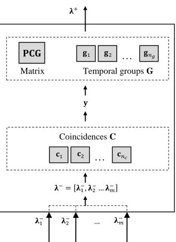
The internal structure of an intermediate node is shown in Fig. 3. The node maintains: a set of coincidences ;
a set of temporal groups (or simply groups) ; a matrix .
Fig. 3. An intermediate node working in inference mode.
3.2.1 Coincidences
Each coincidence is a sort of prototype pattern that spans a portion of the image corresponding to the node receptive field (i.e., small at low levels and large at high levels). Coincidences are used to perform a spatial analysis of input patterns and to find out spatial similarities. However, the coincidence structure depends on the node level: if is an intermediate node at level 1 (hence its child nodes are input nodes), a coincidence corresponds to a
small image patch. An example of coincidence graphical representation in a level 1 node is shown in Fig. 4 (left).
Coincidences C
Temporal groups G
Matrix
… …
8 Note that the coincidence dimensionality is the same as the input message (i.e., the sum of the dimensionality of all the input messages coming from child nodes);
if is an intermediate node at level 2 (hence its child nodes are intermediate nodes), a coincidence can be
conceived as a feature selector: each element is the index of a single temporal group among the groups of
The dimensionality of coincidences is . Although a graphical representation is here
meaningless, a simple numerical example can help understanding: if has 4 child nodes and , then selects: group 5 from child 1, group 3 from child 2, group 1 from child 3 and group 1 from child 4.
3.2.2 Temporal groups
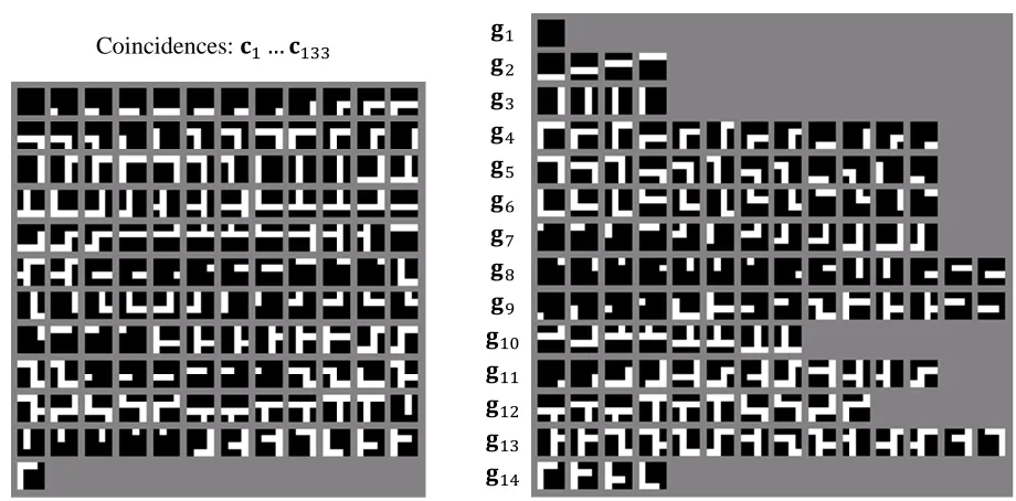
A serious drawback of spatial-similarity-based pattern recognition is that slight variations of the input pattern can produce relevant changes in the feature representation. For example, let us consider the pixel level representation of a short vertical bar (one pixel thick): the right (or left) movement of just one pixel is enough to dramatically reduce the spatial similarity with the original pattern. A temporal group (or simply group) is a subset of coincidences, that could be spatially quite different each from the other, but that are likely to be originated from simple variations of the same pattern. An example of level 1 temporal groups is shown in Fig. 4 (right). The name “temporal”, as it will become clearer in Section 4, depends on the fact that HTM exploits temporal smoothness to create temporal groups; in other words, patterns that are presented to the network very close in time, are likely to be variants of the same pattern that is smoothly moving throughout the network receptive field.
Fig. 4. Coincidences and temporal groups in a level 1 intermediate node trained on line-drawing patterns. Each of the 133 coincidences (on the left) is a 16=4×4 dimensional vector. On the right, graphical representation of 14 temporal groups (one per row). Group denotes a horizontal (and a vertical) bar at different positions within the node receptive field. Groups and correspond to four different types of corner. As explained in Section 4, HTM groups are not hardwired, but are the result of an unsupervised learning process.
Coincidences:
Groups:
9 3.2.3 PCG
is a matrix: element denotes the conditional probability of coincidence given the group , or, in other words, the relative probability of occurrence of coincidence in the context of group
. Hence, for each group , .
3.2.4 Inference steps
Inference in an intermediate node can be decomposed in the following steps (see Fig. 3):
1. Composition of input message: a single input message is obtained as juxtaposition of the
input messages from the child nodes. The dimensionality d of is the sum of
dimensionalities. In general dimensionality can vary across the child nodes.
2. Computation of densities over coincidences: vector is composed by the conditional densities of the evidence given the coincidences: . Intuitively each can be conceived as the activation level
of coincidence when the node input is . computation depends on the node level:
o if is an intermediate node at level 1 (hence its child nodes are input nodes), the input message is essentially
an image patch and coincidences are prototype image patches. In this case encodes the spatial similarity between two image patches and can be conveniently computed as a Gaussian distance:
(1)
where σ is a parameter controlling how quickly the activation level decays when deviates from . Fig. 5 shows an example of coincidence activations;
o if is an intermediate node at level 2 (hence its child nodes are intermediate nodes), the input message is a
probability vector (see point 4 below). In this case is proportional to the probability of co-occurence of sub-evidences (each sub-evidence coming from a child), in the context of . Assuming the sub-evidences to be independent the probability is obtained by product rule:
(2)
where is the element at position in input message from .
For example, if has 4 child nodes, , ,
, and , then ;
For numerical stability (i.e., to avoid that probabilities become too small as we move up in the hierarchy) it is
preferable to normalize such that . This normalization does not alter the HTM behavior.
3. Computation of densities over groups: the conditional density over a group (which intuitively can be
conceived as the activation level of group ) can be obtained by probability marginalization over the group
coincidences:
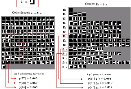
10 where the assumption holds because the knowledge of is irrelevant for the estimation of density in the context of . Fig. 5 shows an example of group activations.
4. Composition of output message: the output message , whose dimensionality is , is simply composed by the conditional densities over the groups: .
Fig. 5. This example shows, in the context of Fig. 4 intermediate node at level 1, the top 3 coincidence activations and the top 3 group activations produced by the input message graphically represented in the box located in the top-left part of this figure. In particular, even if the input patch is not identical to any of the node coincidences, it activates the three spatially closest coincidences. Group activations provide some generalization by associating the input patch to a corner-type pattern, independently of its precise location in the node receptive field.
3.3
OUTPUT NODES
The output node works as a pattern classifier. Its internal structure is shown in Fig. 6: the input part of the node is identical to an intermediate node, whereas in the output part group data are replaced by class data. The node maintains:
a set of coincidences ;
a prior probability vector [ where are the problem classes; a matrix .
Coincidences:
Groups:
top 3 coincidence activations
top 3 group activations
11 Fig. 6. The output node working in inference mode.
3.3.1 Coincidences
Output node coincidences are identical to intermediate node ones (see Section 3.2.1). However, except for
degenerate cases where the network has no intermediate levels, the level of output node is 2 and therefore coincidences at this level work as feature selectors.
3.3.2 Prior class probabilities
In all pattern classification problems, the knowledge of class prior probabilities allows to improve classification
accuracy according to Bayes theory. In HTM prior class probabilities are computed at training time.
3.3.3 PCW
is a matrix: element denotes the conditional probability of coincidence given the class , or, in other words, the relative probability of occurrence of coincidence in the context of class
. Hence, for each class , .
3.3.4 Inference steps
Inference in the output node can be decomposed in the following steps (see Fig. 6): 1. Composition of input message: identical to intermediate nodes (see Section 3.2.4).
2. Computation of densities over coincidences: identical to intermediate nodes (see Section 3.2.4).
Coincidences C
Prior class prob. Matrix
…
12 3. Computation of densities over classes: the conditional density over a class (which intuitively can be
conceived as the activation level of class ) can be obtained by probability marginalization over the class
coincidences:
(4) where the assumption holds because the knowledge of is irrelevant for the estimation of density in the context of .
4. Computation of class posterior probabilities: according to Bayes theorem, class posterior probabilities can be
obtained as:
. (5)
5. Composition of output message: the output message , whose dimensionality is , is simply composed by the
class posterior probabilities: , where .
4.
NETWORK TRAINING
With networktraining we denote a batch procedure aimed at computing: (i) coincidences , groups and
matrix for all intermediate nodes; (ii) coincidences , priors and matrix for the output node. Once training is finalized all network nodes are switched in inference mode and the network can start classifying unknown patterns.
HTM training requires a training set , where is a pattern (e.g., a grayscale
image) and the corresponding class. Intermediate levels are trained in unsupervised mode (i.e., pattern classes are not used), whereas the output node is trained in supervised mode. HTM training is performed level by level, from to ; (input level) does not require any training. When training nodes at level , all the network nodes at
previous levels, whose training was already finalized, work in inference mode. In Section 4.2 we will present the HTM training procedure in details, but before it is necessary to understand how training sequences are generated (Section 4.1).
4.1
TRAINING SEQUENCES
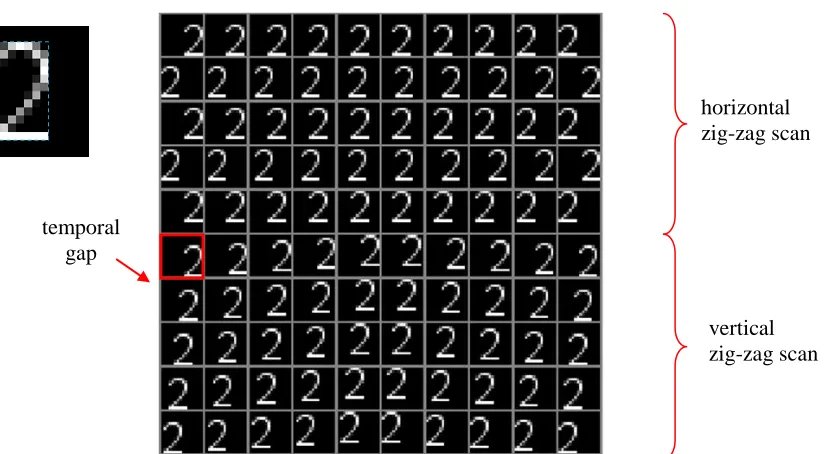
Training an intermediate level requires to expose the network to a sequence of patterns. Such a sequence can be obtained by smoothly moving each training pattern across the network visual field. Since consecutive patterns in the sequence are close in time we can expect they are characterized by minor changes in terms of geometric (e.g., translation, rotation, scale, etc.) and photometric (e.g., brightness, color, etc.) features. Although different strategies can be designed to extract a sequence of temporally close patterns from a training set , a baseline
implementation is as follows: for each pattern perform two scans (an horizontal zig-zag followed by a
13 (temporally) group variants of the same pattern where the bar occurs at slightly different vertical positions. A full training sequence can be obtained by concatenating sequences generated by single training patterns. In general, in a training sequence we can have discontinuities, denoted as temporal gap (see Fig. 7). Temporal gaps occur when we abruptly move a pattern to a distant position to start a new scan or when the training pattern changes (e.g., we stop moving and start with ).
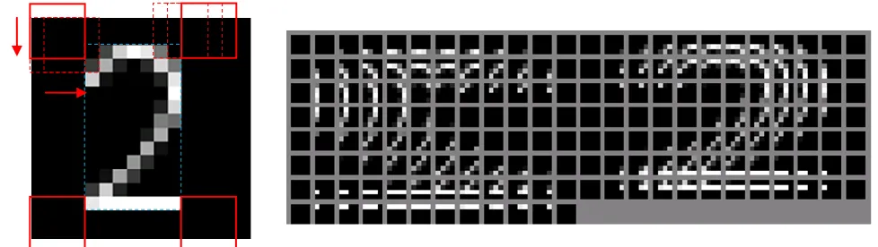
Fig. 7. An example of sequence obtained by the single 16×16 training image shown on the top-left (the foreground object it contains is highlighted with a dashed light blue rectangle). The first pattern, at the beginning of the second scan, is not obtained as a small movement of its predecessor in the sequence, hence it is marked as temporal gap.
Intermediate levels can operate in a special mode (denoted as node sharing): in this configuration all the level nodes share the same coincidences , groups and matrix. When HTM are used for visual pattern recognition, node sharing is typically used for the bottom levels in the hierarchy (e.g., level 1 and/or level 2), whose nodes are expected to learn primitives such as bars, corners, etc. that can occur at any position in the image. Node sharing forces all the nodes of the level to respond in the same way to identical stimuli4. For levels working in shared mode, it is sufficient to train just one node (denoted as master node), and then cloning5 , and of the master node for all the other level nodes. When training a master node, the whole foreground object should be moved across the master node receptive field. In general this require to extend the movement of the foreground object outside the pattern boundaries6. A convenient strategy to generate such a sequence is shown in Fig. 8.
Finally, to train the output node it is sufficient to expose the node to single training patterns with associated class labels (in fact, no temporal information are processed by the output node). However, if the network is required to
4 this is in analogy with early regions (e.g., V1 and V2) in the visual cortex.
5 in practical HTM implementations, cloning is accomplished by using pointers to the master node data structures.
6
note that Fig. 7 sequence does not allow the whole foreground object to be moved over the receptive field of a single (master) node. In fact, let us consider a
level 1 master node with a receptive field of size 4×4: there is no 4×4 subwindow of the 16×16 image over which the entire foreground object is moved.
horizontal zig-zag scan
vertical zig-zag scan temporal
14 recognize patterns independently of their position (translation invariance), each training pattern must be presented at different positions. In practice, we can use training sequences like that reported in Fig. 7, but unlike for intermediate nodes, here only a single scan (either horizontal or vertical) is necessary.
Fig. 8. A convenient way to create the pattern sequence needed to train a master node, is to slide a window (whose size matches the node receptive field) across the foreground object. The example shows the sequence generated by an horizontal zig-zag scan.
4.2
OVERALL TRAINING
A pseudo-code implementation of HTM training is here provided:
HTM Training
Reset coincidences // for all network nodes set
for each level
{ = Training Sequence for Level from // see Section 4.1
= Get First Pattern from // is the label of the pattern class
while (I is not null)
{ Expose I to
for each Level
Do Inference // see Sections 3.1 and 3.2.4
Train on // expanded below
= Get Next Pattern from }
Finalize Training on // expanded below
}
where:
Train on
if ( ) // output level
Train Output Node on // see Section 4.4
else if ( is a node sharing Intermediate level)
Train Intermediate Node on // see Section 4.3 (we assume that is the master node)
else // intermediate level (no node sharing)
{ for each Node
Train Intermediate Node on // see Section 4.3
15 and
Finalize Training on
if ( ) // output level
Finalize Output Node Training // see Section 4.4
else if ( is a node sharing Intermediate Level)
{ Finalize Intermediate Node Training // see Section 4.3
for each node Clone from
}
else // intermediate level (no node sharing)
{ for each Node
Finalize Intermediate Node Training // see Section 4.3
}
4.3
INTERMEDIATE NODE TRAINING
The procedure Train Intermediate Node on , reported below, assumes that I has been presented to the network (level ) and inference has been already performed until level . Hence messages are available from the child nodes of .
Train Intermediate Node on
Compose Input Message // see 3.2.4, point 1
if ( // node at level 1 → is an image patch
{ // select the coincidence closest to , as candidate active coincidence
if ( ) // none of the existing coincidences is spatially representative of
{ // increase number of coincidences
= // add to as a new coincidence
// the active coincidence is the new one
} }
else // node at level ≥ 2 → is a probability vector
{ = Indices of Child Winning Groups in // see Equation 6
// select the coincidence closest to , as candidate active coincidence
if ( ) // none of the existing coincidences is spatially representative of
{ // increase number of coincidences
= // add to as a new coincidence
// the active coincidence is the new one
} }
// number of times was the active coincidence during training
if ( is not a temporal gap pattern)
// updates Temporal Activation Matrix
// remember the active coincidence for next step
16 the active coincidence is the spatially closest coincidence to the node input. If all existing coincidences are too
dissimilar from the input (with respect to a level specific threshold ), then a new coincidence is created and selected as active coincidence. Selecting and bringing forward only one coincidence, implements a winner take all criterion that is in contrast with the continuous criterion used during inference, when the activation of all coincidences are taken into account for the computation of group activations (see Equation 3). It is worth noting that such an asymmetrical approach (winner take all for learning vs continuous for inference) is not atypical, and proved to be quite effective in training other deep architectures [15][30];
is a vector of indices of child winning groups. Index is the group index, within the groups of child node , which obtained maximum activation. Let be the number of groups in , and
be the element of vector , then:
(6)
Here too a winner take all criterion is adopted. In fact, only the index of the most active group within each child node is considered. Again, this is in contrast with the continuous criterion used during inference where the activations of all child groups are used to compute coincidence activations (see Equation 2);
counts the number of differences between indices at corresponding positions in the two vectors. For example, if and , then ;
A scalar is maintained for each coincidence to count the number of times was active during the node training. When finalizing node training these values will be used to quantify coincidence relevance;
, denoted as Temporal Activation Matrix (or TAM), is an matrix, used to keep track of coincidences that have been activated in succession, and thus are good candidates to form a temporal group. When finalizing node training will be used to compute temporal groups and . For simplicity of presentation, in the above pseudocode update is performed by looking only one step back in time (i.e., through ). In general, better performance can be achieved by considering steps back: let be the index of the active coincidence steps back in time, then:
for each
where linearly decreasing weights are here used to update as the time gap increases.
17 Finalize Intermediate Node Training
Forget Rare Coincidences // coincidence such that are removed from
Compute Coincidence Priors // see Equation 7
Make Symmetric // after this step:
Normalize by Rows // after this step: , see Equation 8
Temporal Grouping // determine groups from clustering, see Section 4.3.1
Compute // see Section 4.3.2
where:
forgetting rare coincidences can be useful to reduce the number of coincidences; in fact, deletion of rarely
activated coincidences usually has a minor impact on the network classification accuracy; to make symmetric the upper diagonal part is summed to the lower diagonal part 7:
for each pair
Making symmetric allows coincidences that occurred close in time to be grouped independently of the activation order. Therefore a pattern moving left-to-right across a node receptive field yields to the same groups as the same pattern moving right-to-left;
coincidence priors can be simply obtained by normalizing the number of times coincidences have been activated
during training:
(7)
values are proportional to the probability of (close in time) co-occurrence of coincidences. A simple
normalization by rows makes values true conditional probabilities:
for each
After normalization:
(8)
where means that was active at time , and , for each . Note that after
normalization is no longer symmetric.
Some further definitions are useful before discussing group computation:
Equation 8 asserts that is the probability that the next active coincidence will be if the current active coincidence is ; in other words, denotes the temporal connection of the (ordered) pair , ;
the temporal connection of a single coincidence is the probability that the next active coincide will be independently of the currently active coincidence, and can be obtained from 8 by marginalization:
(9)
where we assume that are the prior probabilities obtained from Equation 7, and therefore:
7 throughout this paper, for Equations that require updating a whole matrix/vector by overwriting the same matrix/vector, we denote the target with the
18
(10)
the temporal connection of a group is the average temporal connection between any two coincidences belonging to the group. Let be the number of coincidences in , then:
(11)
4.3.1 Temporal Grouping by T Clustering
A temporal group is a set of coincidences that are likely to occur close in time. Partitioning coincidences into
a set of disjoint groups , can be formulated as a clustering problem aimed at maximizing the functional:
(12)
subject to the constraints:
for each (13)
(14)
for each (15) Equation 13 asserts that groups must be disjoint, equation 14 that all the coincidences must be assigned to groups and Equation 15 sets a maximum group size. Maximization of 12 leads to maximize the average group temporal connection, that is the within group temporal connections among coincidences.
Clustering is one of the most studied problem in pattern recognition and machine learning [31] and hundreds of algorithms have been proposed in the literature. The clustering problem at hand has some peculiarities: (i) we can easily compute similarity between any pair of coincidences, but there is not an efficient way to compute the centroid of a set of coincidences (this makes the application of k-means like approaches critical); (ii) the number of coincidences and groups can be quite large in practical applications, so we need computationally efficient approaches; (iii) we do not care too much about the optimality of the solution since HTM is robust enough with respect to suboptimal grouping. For this reasons an ad-hoc (computationally efficient) greedy algorithm, here denoted as Default temporal clustering, was introduced in [32]:
Default Temporal Clustering
// a flag is maintained to denote coincidences already assigned
while (not all coincidences have been assigned) {
// select the non assigned coincidence with highest temporal connection
// initialize a new list with a single coincidence
// this is a cursor used to scan elements by their position
while ( ( ) // until scan is completed or group is too large; ( is the list length
{ // get coincidence at position in the list
19
}
// create a new empty group and add it to
for each // add the first coincidences in to the new group
{
// mark it as assigned
} }
where:
selects the coincidences with highest temporal connection
with , excluding coincidences already assigned. Selected coincidences are added to , by inserting them at the end of the list and by excluding coincidences already present in the list. A typical value for is 3. The default temporal clustering algorithm runs by creating one group at each time. The group seed is a single highly connected coincidence, to which its coincidence are associated; group growing is recursive, i.e., each newly associated coincidence will cause its coincidences to be associated as well. Recursion terminates: (i) naturally, when the coincidences of all the coincidences in the list are already in the list; (ii) forcedly, if the list length exceeds . Some nice graphical examples of group growing are shown in [32]. Temporal grouping shown in Fig. 4 has been created with the default temporal clustering algorithm. A different algorithm, based on Agglomerative Hierarchical Clustering, was proposed in [1].
4.3.2 PCG Computation
denotes the conditional probability of coincidence given the group . The computation of matrix is performed in two simple steps:
1.
, for each
2. , for each
The former step sets the conditional probability as the coincidence prior in case the coincidence belongs to the group.
The latter is a within group normalization aimed at guaranteeing, for each group , that
4.4
OUTPUT NODE TRAINING
Training the output node during pattern presentation is very simple:
Train Output Node on
... // the first part, aimed at selecting/creating the active coincidence , is identical to Intermediate Node Training, see Section 4.3.
20 A few steps are required to finalize the output node training:
Finalize Output Node Training
Forget Rare Coincidences // coincidence such that are removed from
Compute Class Priors // see Equation 16
Normalize // see Equation 17
where:
is the total number of times coincidence has been active independently of the pattern class;
these values are here used to forget rare coincidences;
class Priors are computed by marginalization and normalization:
(16)
normalization is aimed at guaranteeing, for each class , that
, for each . (17)
5.
NEW TRAINING
ALGORITHMS
In this Section we introduce new training techniques: in particular, Section 5.1.1 presents a new temporal clustering algorithm, Section 5.1.2 introduces a fuzzy grouping approach, and finally in Section 5.1.3 we discuss computational issues and show how activation buffering can markedly reduce training time.
A new constructive definition of is fundamental for the discussion hereafter. Let be a temporal grouping solution and be a normalized temporal activation matrix (see Equation 8), then:
(18)
where:
, since given , the knowledge of is irrelevant to determine ;
is computed as the relative prior probability of (see Equation 7) over the total prior probability of coincidences belonging to group :
.
Hence Equation 18 becomes:
(19)
It can be simply proved that, for each group :
(20)
21
.
According to Equations 18 (and 19) the conditional probability of a coincidence given a group can be
conceived as the probability that the next active coincidence will be if the currently active coincidence is one of the coincidences of the group . It is worth noting that Equation 19 allows to compute the degree of membership of
a coincidence to a group either if the coincidence belongs to the group or not. Equation 19 also allows to define the stability of a group :
(21)
is the probability that if the currently active coincidence belongs to then the next active coincidence will also belong to . It can be simple proved that always lies in [0,1], where 1 means maximum stability; in fact, is smaller than or equal to the summation in Equation 20.
It should be noted that the definition of group stability is quite similar to that of group temporal connection (see Equation 11): the only difference is that to compute group stability we make use of prior probabilities to weight values non uniformly.
5.1.1 MaxStab Temporal Clustering
The default temporal clustering approach introduced in Section 4.3.1 indirectly maximizes functional (Equation
12) by forming groups with high internal values. The algorithm here introduced performs a more direct maximization of the average group stability, expressed by the functional:
(22)
subject to the constraints 13, 14 and 15.
MaxStab Temporal Clustering
// a flag is maintained to denote coincidences already assigned
while (not all coincidences have been assigned) {
// select the non assigned coincidence with highest temporal connection
// create a new empty group and add it to
do
{
// get coincidence that most increases group stability
}
22 where:
computes the delta stability resulting from the inclusion of in .
MaxStab creates one group at each time starting from a single highly connected coincidence. The group is then expanded by associating, step by step, the coincidence that most increases the group stability. The expansion continues while: (i) the increase in stability is larger than a given threshold computed as , and (ii) the group size is smaller than .
Because of the similarity between group stability and temporal connection both and maximization are expected to give similar results. However in our experiments, MaxStab usually leads to an higher average group stability (Equation 22) with respect to the default temporal clustering of Section 4.3.1, and this often results in better classification performance. On the other hand, since HTM networks are quite robust with respect to suboptimal grouping the accuracy improvement is often marginal. A graphical comparison of the solutions obtained with the two algorithms is shown in Fig. 9.
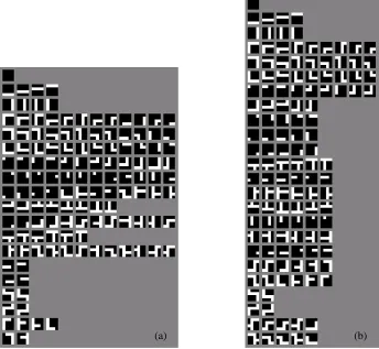
Fig. 9. Two temporal groupings over the coincidences of Fig. 4 (left) starting from the same temporal activation matrix: (a) clustering was performed with the default temporal grouping algorithm with parameter values: , . The first group, i.e., that containing a single empty patch, was hardcoded; in fact, we noted that for line drawing classification, in case of perfectly clean background, this often leads to better accuracy. The average group stability obtained is (b) clustering was performed with MaxStab algorithm with parameter values: , . Unlike for the default algorithm, no group was hardcoded here, since MaxStab can create groups with a single element. The average group stability obtained is . Finally it should be noted that groups in (b) are better balanced and that while in (a) group growing was terminated in 8 cases by the maximum group size constraint, in (b) group growing always terminated naturally because of the threshold imposed by .
23 5.1.2 Fuzzy Grouping
In Section 4.3.1, Equation 13 requires the groups to be disjoint (i.e., no coincidence can be part of more than one group) and Equation 14 requires all coincidences to be assigned to one group. In real applications, rarely clusters can be clearly identified and even for optimal solutions some patterns can lie near the boundaries of two of more clusters. Forcing patterns to be member of only one cluster can lead to ambiguity. For this reason in many pattern recognition applications, probabilistic or fuzzy clustering, such as fuzzy-k-means [33] or Expectation-Maximization [34] is preferred to exclusive clustering. In the following we will relax Equation 13 and 14 constraints; this will lead to the formation of partially overlapped groups from which we will derive in a novel way. Some steps in this direction (non exclusive grouping) were pioneered by Greg Kochaniak (unfortunately a formal description of his approach is not available), but his temporal grouping implementation was quite different from the fuzzy grouping approach here introduced.
To implement Fuzzy grouping, the last two steps of the Finalize Intermediate Node Training algorithm in Section 4.3 must be replaced with the following five sequential stages (previous steps remain unaltered):
1. Compute initial groups with a clustering algorithm enforcing Equation 13 and 14. This initial clustering solution can be computed with the default algorithm described in Section 4.3.1 or with the MaxStab algorithm described in Section 5.1.1.
2. Remove small groups and groups with low stability. Groups with less than coincidences are expected to bring limited generalization, so they are removed. Analogously, groups such that are removed since their elements are not enough temporally close each other. At this stage coincidences of deleted groups remain orphans (Equation 14 is no longer enforced).
3. Computation of . Each element is calculated according to Equation 19.
4. Group extension. Given a group , coincidences already belonging to at the end stage 2, are denoted as
primary coincidences, whereas coincidences added subsequently (i.e., during this phase) are denoted as
secondary. Since primary coincidences contributed to the group formation they are expected to be the most representative for the group. However, other coincidences not belonging to the group could be temporally close to coincidences in the group: we allow a coincidence to be added to a group as secondary coincidence if
is high. However, instead of explicitly thresholding , group extension is accomplished as:
Group Extension to Secondary Coincidences
for each
{
while ( // we want to add only to the top% groups (default value for )
{
// select the temporally closest group, excluding those already considered
// to avoid selecting again
24
// is added to as secondary coincidence
} }
At the end of this stage Equation 13 is no longer enforced.
5. Cleaning and Normalization of
, for each .
This step clears a value, computed at stage3, if does not belong (neither as primary nor as secondary) to group .
, for each
This step is necessary, after cleaning, to ensure that for each group , .
It is worth noting that fuzzy grouping could be implemented without group extension (stage 4) and cleaning/normalization (stage 5), since, at the end of stage 3, matrix is already consistent. However, the proposed implementation leads to a sparse (e.g., only a minor portion of its element are not 0) which is preferable for both robustness (as confirmed by experimental results) and computational efficiency. In the rest of this paper we will denote the temporal grouping introduced in Section 4.3.1 as exclusive grouping in order to distinguish it from the fuzzy grouping here proposed. Fig. 10 shows an example of fuzzy grouping and compares it with the exclusive grouping solution from which it was derived.
5.1.3 Activation Buffering
In Section 4.2 we explained that HTM training is performed level by level: while training level , all the nodes of previous levels work in inference mode. Therefore all the patterns in the training sequence used to train level must be processed (i.e., inference) by all the levels . For huge training sequences this (lower level)
processing can be computationally demanding thus leading to long training time. However, since the training sequences used to train the different levels are usually generated from the same training patterns, buffering the node responses (i.e., the group activations) allows re-processing of the same patterns to be avoided. This idea is derived by an HTM implementation developed by Greg Kochaniak.
Activation buffering implementation details depend on the training strategy and in particular on the composition of the training sequences. In the following we assume that training sequences are created as described in Section 4.1 where patterns in each training sequence are obtained by one or more exhaustive scans over the training set patterns (see Fig. 7 and Fig. 8). Let be a training set pattern, then is the pattern
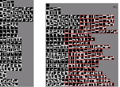
25 Fig. 10. (a) The exclusive grouping solution reported in Fig. 9.b is characterized by an average group stability . (b) Fuzzy grouping solution obtained starting from groups in (a) and with parameter values: ,
, . Two groups have been deleted because of .
Coincidences enclosed inside red frames are secondary coincidences added during group extension. It can be noted that many of the secondary coincidences can be obtained by small translations of primary coincidences in the same group. Here the average group stability grows to , and, even if the average group length increases from 5.5 to 14, the percentage of non-zero elements remains quite small (10.5%).
no node sharing. For each node of level and for each pattern the index of the winning
group (i.e., the most active group) is stored in a buffer: . When training nodes of level , indices of child winning groups ( ,see Equation 6) are composed by directly accessing the buffer
without any lower level pattern re-processing.
node sharing. Only the master node is trained. In this case, the node reference is always 1, so the buffer entries are . When training nodes of level the child winning group index of each
non master node can obtained by accessing the buffer at a position that depends, not only on the current scan offset, but also on the relative position of with respect to the master node (in practice, the activation of a non master node is derived from the master node activation upon receptive field shifting).
Two types of activation buffering, denoted as normalBuffering and fastBuffering, can be implemented:
normalBuffering results are identical to the non-buffering case. Buffering is performed at the end of node training
when the entire training sequence is presented again to the network and inference is carried out through previous (a)
26 levels . However, NormalBuffering is effective only for levels operating in node sharing mode; making
it advantageous also for "no node sharing" levels would be very complex and space-demanding.
fastBuffering results are usually slightly different with respect to the non-buffering case. Buffering is carried out
in two stages: (i) during the training of level , the winning coincidence indices (i.e., the most active coincidence indices) are buffered. At the end of training, once has been computed, winning coincidence indices are batch converted into winning group indices. This is an heuristic step (leading to a loss of information) because it ignores the contributions of the non-winning coincidences to the computation of group activation levels (see Equation 3). However, from experimental results (refer to Section 6) we noted that fastBuffering is not only more efficient, but sometimes is also more accurate than normalBuffering, and in general, even when it is less accurate, the accuracy drop is small.
6.
P
ATTERN CLASSIFICATION EXPERIMENTSIn this Section we present several experimental results on pattern classification problems: Subsection 6.1 introduces the three datasets used in the experiments; in Subsection 6.2 we discuss HTM training, tuning and parameterization and we compare the new training algorithms of Section 5 with the default implementation reported in Section 4; finally, in Subsection 6.3 HTM is compared with other pattern recognition approaches.
6.1
DATASETS
For this study we selected three different pattern classification problems: SDIGIT, PICTURE and USPS. In our opinion, these three datasets constitute a good benchmark to study invariance, generalization and robustness of a pattern classifiers. However, in all the three cases the patterns are small black-and-white or grayscale images (32×32 or smaller). Even if HTM was already applied with success to object recognition problems with larger color images (see [3][11]) our current implementation need to be further enhanced to be able to efficiently works with large patterns. As discussed in Section 7, part of our future efforts will be dedicated to the demonstration of HTM capabilities on typical object recognition benchmarks such as CalTech and Pascal VOC datasets [35].
6.1.1 SDIGIT
SDIGIT is a machine-printed digit classification problem where just a single (16×16 pixels, 8-bit grayscale) image, called primary pattern, is provided for each of the 10 digit classes, and a number of variants are generated by geometric transformations of the primary patterns. By explicitly controlling the size and the amount of variation in both the training and the test set we can study specific characteristics of HTM related to training, generalization/invariance, robustness. With we denote a set of
patterns, including, for each of the 10 digits, the primary pattern and further patterns generated by simultaneous scaling and rotation of the primary pattern according to random triplets where
27 The creation of a test set starts by translating each of the 10 primary
pattern at all positions that allow it to be fully contained (with a 2 pixel background offset) in the 16×16 window thus obtaining patterns; then, for each of the patterns, further patterns are generated by transforming the pattern according to random triplets ; the total number of patterns in the test set is then . Fig. 11 shows an example of test set generation.
Fig. 11. SDIGIT: 10 patterns for each class extracted from a test set . Note the large intra-class variation because of relevant rotation and scale changes; also note that some patterns of different classes appear to be very similar (e.g., rotated "1" and "7", small "5" and "6").
6.1.2 PICTURES
This is a difficult line-drawing classification problem introduced in [1]. The dataset can be obtained from [5]. Patterns are 32×32 pixels, 1-bit (i.e., black and white) images belonging to 48 classes, including: characters, stereotyped animals and simple objects. The training set is constituted by 453 images; pattern distribution over classes in unbalanced but all classes have more than one pattern. The test set is composed by 8,941 patterns which represent distorted versions of the training set ones. Distortion includes geometric change, line thickness change, noise (i.e., randomly flipped pixels), disconnection/cancellation of parts; some of the patterns are so severely distorted that also human classification is challenging. Fig. 12 shows some examples. A reduced version of PICTURE problem, denoted as PICTURE-, can be obtained by considering only the first 8
classes: in particular, contains 100 patterns and contains 2,000 patterns.
6.1.3 USPS
USPS is a well known handwritten digit classification problem [36], largely used in the scientific literature as a benchmark for pattern recognition and machine learning approaches. USPS patterns are 16×16 pixels, 8-bit grayscale images; the training set and test set contains 7,291 and 2,007 patterns respectively. Fig. 13 shows some examples. With we denote a subset of the training set composed by the first
28 Fig. 12. Two examples per class extracted from (a) and (b) .
Fig. 13. Ten examples per class extracted from (a) and (b) .
6.2
HTM ANALYSIS
Designing an HTM architecture and finding optimal values for the numerous parameters controlling the network learning and inference is not a trivial task. Furthermore, as for many other pattern recognition approaches, the optimal architecture and parameter values are problem dependent and a proper parameter tuning can lead to a relevant performance improvement. Fortunately HTM is quite robust with respect to its parameterization and
(b) (a) (a)
29 performance just nicely degrades as parameters drift away from their optimal values. In our experimentation we tried to fix, as much as possible, the network architecture and the parameter values independently of the problem. This could lead to suboptimal accuracy, but in general allows to control data overfitting, especially when a validation set (disjoint from the test set) is not available to tune parameters.
6.2.1 Parameter selection
Table I list the parameter values that we found to be appropriate for all the classification problems addressed in this work, while Table II includes dataset specific parameter values.
All the HTM used are four-level networks: two intermediate levels perform both spatial and temporal analysis; the output level performs a further spatial analysis and then classifies the pattern. Some experiments have been carried out with three- and five-level networks too; although with proper parameterization these architectures can perform well (sometimes better than a four-level HTM), a four-level architecture demonstrated to be an optimal choice for input patterns of size 16×16 and 32×32. As reported in Table II, node arrangements across the four levels is 16×16 → 4×4 → 2×2 → 1 (as in Fig. 1 example) for SDIGIT and USPS, and 32×32 → 8×8 → 4×4 → 1 for PICTURE.
Level 1 always operates in node sharing mode since its nodes are expected to learn basic features that are somewhat independent of the position within the network receptive field. Level 2 also operates in node sharing mode for PICTURE while level 2 node sharing is not activated for SDIGIT and USPS since in these cases pattern translations across the input window is more limited and nodes experience sub-patterns that are position dependent.
Common parameter values
Level 0 (Input) Level 1 (Intermediate) Level 2 (Intermediate) Level 3 (Output)
Default Temporal Clustering
MaxStab Temporal Clustering
Default Temporal Clustering
MaxStab Temporal Clustering
Table I. Common parameter values for all the HTM networks used in our experiments. Optimal parameters for both Default Temporal Clustering and MaxStab Temporal Clustering are reported. Parameter is used only if Fuzzy Grouping is activated.
SDIGIT
Level 0 (Input) Level 1 (Intermediate) Level 2 (Intermediate) Level 3 (Output)
16×16 4×4
MaxStab Temporal Clustering
2×2