A non-simultaneous dynamic ice-structure interaction model

1 A Non-simultaneous Dynamic Ice-structure Interaction Model

1

Xu Ji*, Dale G. Karr**, Erkan Oterkus*** 2

3

* Department of Naval Architecture, Ocean and Marine Engineering, University of Strathclyde 4

100 Montrose Street, Glasgow, G4 0LZ, United Kingdom 5

Phone: +44 (0)141 5484094 6

e-mail: [email protected] 7

8

** Department of Naval Architecture and Marine Engineering, University of Michigan 9

2600 Draper Drive, Ann Arbor, Michigan, 48109, United States of America 10

Phone: +1(734) 764-3217 11

e-mail: [email protected] 12

13

*** Department of Naval Architecture, Ocean and Marine Engineering, University of Strathclyde 14

100 Montrose Street, Glasgow, G4 0LZ, United Kingdom 15

Phone: +44 (0)141 5483876 16 e-mail: [email protected] 17 18 Abstract: 19

To simulate non-simultaneous ice failure effects on ice-structure interaction, an extended dynamic Van der Pol 20

based numerical model is developed. The concept of multiple ice failure zones is proposed to fulfil non-21

simultaneous crushing characteristics. Numerical results show that there is more simultaneous force acting on 22

all segments at lower ice velocity and there is more non-simultaneous ice failure at higher velocity. Variations 23

of force records show a decreasing trend with increasing ice velocity and structural width. These effects can 24

be attributed to the assumption that the size of ice failure zone becomes smaller with increasing ice velocity, 25

which increases the occurrence of non-simultaneous ice failures. Similarly, the decreasing size of ice failure 26

zone as velocity increases is explained as the reason of different ice failure modes shifting from large-area 27

ductile bending to small-area brittle crushing. The simulation results from a series of 134 demonstration cases 28

show that the model is capable of predicting results at different ice velocities, structural widths and ice 29

thicknesses. In addition, analysis of the ice indentation experiments indicates that the mean and minimum 30

effective pressure have an approximately linear relationship with ice velocity, which testified the assumption 31

on variations of ice failure zone in the model. 32

33 34

Keywords: 35

Non-simultaneous failure; Ice-structure interaction; Ice failure zone; Van der Pol equation. 36

NOMENCLATURE 37

i

L

Ice failure length of each ice strip (m)

c Constant distributed normally with mean

µ

and variance

σ

_s2

H

Ice thickness (m)

0

2

0

K

Reference stiffness (kN m-1)

K

Structural stiffness (kN m-1)

strip

N

Number of ice strips

i

W Width of an ice failure zone (m)

M

Mass of the structure (kg)

C Damping coefficient (kg s-1)

ξ Damping ratio

X Structural acceleration (m s-2) X Structural velocity (m s-1) X Structural displacement (m)

T

Time (s)

A

Magnification factor

σ Ice stress (kPa)

D

Structural width (m)

i

q Dimensionless fluctuation variable of each ice strip ,

a ε Scalar parameters that control the qi profile

i

ω

Angular frequency of ice force (rad s-1)

i

f

Ice failure frequency (Hz)

B Coefficient depending on ice properties

i

Y

Velocity of each ice strip (m s-1)

i

Y

Displacement of each ice strip (m)

i

Y

Acceleration of each ice strip (m s-2)

max

σ

Maximum stress at ductile-brittle range (kPa) ,

d b

σ σ

Minimum stress at ductile and brittle range (kPa)

r

v

Relative velocity between ice and structure (m s-1)

t

v

Transition ice velocity approximately in the middle of transition range (m s-1) ,

α β Positive and negative indices to control the envelope profile

𝜇_" Mean effective pressure (kPa)

𝜎" Standard deviation of effective pressure (kPa) 𝐹_% Mean value of ice force (kN)

𝐹_& Standard deviation of ice force (kN)

∆𝜇₍, ∆𝜎₍ The difference between the results from model and experiment for 𝜇( and 𝜎(

1. INTRODUCTION

1

As the study of ice failure has advanced, non-simultaneous failure has gained increasing attention. It can be 2

utilized to explain several well-recognized issues, such as higher localized pressure zone than global pressure 3

3 Kry (1978) proposed an estimation of statistical influence on non-simultaneous failure across a wide structure 1

and divided the ice interaction surface into multiple equivalent zones that are statistically independent of each 2

other. Then Kry (1980) found that ice generally had a more uniform contact with a structure at low velocity 3

and more irregular contact at higher velocity. Ashby et al. (1986) explained the non-simultaneous failure as a 4

size effect resulting from cracks of different lengths having been distributed statistically in ice. Bhat (1990) 5

proposed that ice fails at many self-similar zones like many other fractals in nature and proposed an equation 6

to control the size effect depending on the scale to estimate the irregular ice contact geometry. 7

Sodhi (1998) used segmented indentors to conduct a series of ice indentation tests and found simultaneous 8

failure at low velocity and non-simultaneous at high velocity, and proposed an equation to estimate the 9

decreasing size of ice failure length with increasing indentation velocity. Yue et al. (2009) installed ice load 10

panel on a full-scale monopod platform and found simultaneous ice failure on different panels during lock-in 11

condition. 12

At the same time, many ice-structure interaction numerical models have been developed. Matlock et al. (1971) 13

proposed the very first ice-structure interaction model and many Matlock based numerical models have been 14

developed since then (Huang and Liu, 2009; Karr et al., 1993; Withalm and Hoffmann, 2010). Non-15

simultaneous ice-structure interaction models have been developed based on Matlock model (Hendrikse et al., 16

2011; Yu and Karr, 2014) by extending the single ice strip into multiple strips moving towards the structure. 17

Another method of modelling the interaction process is through utilizing Van der Pol ice force oscillator to 18

control ice force fluctuations (Wang and Xu, 1991). Three distinctive structural response modes and ice-19

induced vibration phenomenon were captured in Ji and Oterkus (2016). Physical mechanism of ice-structure 20

interaction at each stage were discussed based on feedback mechanism and energy mechanism in Ji and 21

Oterkus (2018). 22

In this study, following the concept of Matlock-based non-simultaneous modeling, an extension of Ji and 23

Oterkus (2018) Van der Pol based model is introduced. Apart from the ice velocity and structural stiffness 24

effect on the ice failure, a normally distributed variable is added in the ice failure length equation instead of a 25

constant in the previous model. In addition, the previous one-dimensional single strip ice model is extended 26

to a two-dimensional multiple strips ice model in this study. 27

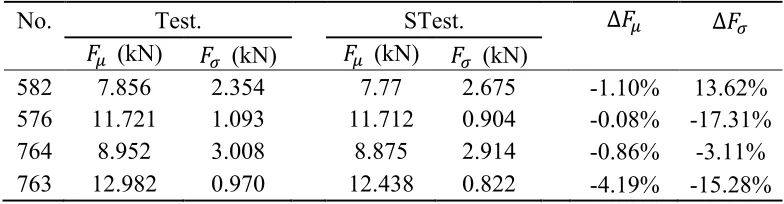
2. EXPERIMENTAL DATA FROM SODHI (1998) 28

Sodhi (1998) listed 159 test results including structural width D, ice thickness H, ice velocity v, mean 29

𝜇₍ and standard deviation 𝜎₍ of the effective pressure across the interaction surface. In Test 582 and 576 as 30

well as Test 764 and 763, they are sharing similar ice thickness and structural width but different ice velocities. 31

In Test 582 and 764 as well as Test 576 and 763, they share similar velocities but different ice thicknesses and 32

structural widths. Therefore, different tests, Test. 582, 576, 764 and 763, are simulated by the numerical model. 33

The time history of ice force and structural displacement are plotted and compared with the time history of 34

experimental results. 35

To use the data more efficiently for blind test later, they are relisted in the Table 1. There are four main sections 36

in total with different D ranging from 50 mm, 150 mm, 250 mm to 350 mm. Each section has several groups 37

of data from (A) to (K). Each group has the ice thickness with 1 mm difference, or rarely with 1.5mm 38

difference. Then each group is sorted from the lowest to the highest ice velocity. There are 25 tests that are 39

not grouped together because of limited similar ice thickness, as shown in grey color in the Table 1. Therefore, 40

134 different tests are simulated by only changing the D,H and v. Then, 𝜇₍ and 𝜎₍ are compared 41

between the numerical simulations and experimental results. 42

[image:4.595.38.277.53.742.2]

4 Table 1. Test configurations from Sodhi (1998).

1

Test D

mm

H

mm

v

mm s-1 𝜇(

MPa

𝜎(

MPa

Group Test D

mm

H

mm

v

mm s-1 𝜇(

MPa

𝜎(

MPa

Group

166 50 25.1 62 2.032 0.243

(A)

399 150 25.5 44 0.933 0.3

160 50 27.3 80 2.307 0.34 398 150 26.6 20 1.69 0.906

165 50 24.8 100 2.12 0.224 391 150 27 20 1.907 0.862

167 50 25 125 1.78 0.291 390 150 27 45 1.029 0.347

164 50 26.3 199 1.504 0.319 410 150 30.6 20 1.869 0.831

(D)

163 50 25.6 300 1.644 0.256 405 150 30 27 2.214 0.967

162 50 26.3 400 1.622 0.263 411 150 30 43 1.077 0.321

161 50 25.7 492 1.915 0.301 404 150 30 43 1.265 0.45

158 50 45.1 47 1.736 0.229

(B)

356 150 32.3 81 1.402 0.4

154 50 44.4 82 1.681 0.229 354 150 32.8 97 1.665 0.544

153 50 45.2 101 1.548 0.237 358 150 31.8 134 1.374 0.357

155 50 44.2 127 1.877 0.265 357 150 32.4 134 1.372 0.287

156 50 43.3 156 1.417 0.307 361 150 30.5 181 1.424 0.231

157 50 43.5 188 1.394 0.408 359 150 31.2 187 1.178 0.245

152 50 45.6 197 1.461 0.188 353 150 32.7 197 1.62 0.236

159 50 45.3 224 1.363 0.25 351 150 33.3 395 2.06 0.197

151 50 43.9 304 1.392 0.247 352 150 33.4 294 1.813 0.223

150 50 45.6 393 1.497 0.231 366 150 45.1 194 1.706 0.38

175 50 69.7 103 2.491 0.555 367 150 46 270 1.959 0.231 176 50 71.1 136 2.509 0.742 364 150 46.2 197 1.819 0.45 362 150 15.3 406 2.405 0.275 363 150 46.8 301 2.186 0.236

388 150 18.8 10 1.62 0.634

(C)

534 250 17.9 48 0.803 0.287

(E)

387 150 18.8 20 0.806 0.25 536 250 17.8 56 0.874 0.226

378 150 18.7 25 0.925 0.288 535 250 17.7 72 0.864 0.207

386 150 18.5 31 1.086 0.306 537 250 18.1 72 0.834 0.384

385 150 18.5 42 0.856 0.239 538 250 17.9 73 0.917 0.167

377 150 18.7 42 0.986 0.287 533 250 18 102 0.893 0.2

376 150 18.7 42 0.91 0.266 521 250 18.2 149 0.997 0.13

373 150 17.3 52 1.012 0.192 532 250 18.1 201 1.026 0.184

375 150 17.6 74 1.055 0.192 540 250 18.1 249 1.123 0.121

374 150 17.6 90 0.915 0.36 531 250 18.2 300 1.158 0.212

375 150 17.6 99 1.144 0.199 539 250 18.1 350 1.257 0.135

371 150 17.8 100 1.114 0.177 549 250 18.5 355 1.234 0.13

372 150 17.8 200 1.263 0.171 548 250 18.4 499 1.319 0.161

369 150 18.5 391 1.462 0.147 516 250 24.8 10 1.58 0.948

(F)

370 150 18 394 1.399 0.167 513 250 24.8 10 1.454 0.597

368 150 18.5 469 1.508 0.178 528 250 25.4 21 1.536 0.791

384 150 19.2 21 0.991 0.331 514 250 24.6 42 0.934 0.382

403 150 24.5 14 2.083 0.769 527 250 25.4 42 1.025 0.421

402 150 24.5 21 1.657 0.724 592 250 23.6 83 0.937 0.253

401 150 25.5 31 0.99 0.344 590 250 24.1 104 1.003 0.195

5

Test D

mm

H

mm

v

mm s-1 𝜇₍

MPa

𝜎₍

MPa

Group Test D

mm

H

mm

v

mm s-1 𝜇₍

MPa

𝜎₍

MPa

Group

591 250 23.8 159 1.055 0.157

(F)

556 250 42.2 6 1.258 0.807

589 250 23.9 202 1.141 0.131 560 250 43.1 219 1.289 0.182

593 250 24 254 1.181 0.116 553 250 44.3 8 1.198 0.819

588 250 24 315 1.212 0.132 552 250 44.3 8 1.38 1.02

587 250 24.5 373 1.246 0.121 760 350 20.3 82 0.835 0.143

(J)

586 250 24.7 408 1.304 0.115 752 350 22.2 100 0.899 0.174

585 250 25.1 465 1.377 0.124 759 350 20.2 156 0.939 0.088

583 250 25.7 490 1.611 0.127 761 350 20.5 157 0.915 0.105

582 250 32.7 102 0.961 0.288

(G)

755 350 20.7 172 0.994 0.094

579 250 33.9 133 1.085 0.214 758 350 20.2 251 1.001 0.095

578 250 33.3 199 1.199 0.162 754 350 20.8 306 1.125 0.093

572 250 34.6 199 1.25 0.277 757 350 20.3 354 1.117 0.085

581 250 33 246 1.236 0.146 753 350 20.8 401 1.17 0.089

577 250 34.2 312 1.291 0.141 751 350 21.1 453 1.214 0.09

580 250 33 356 1.32 0.132 756 350 20.4 459 1.163 0.082

575 250 33.2 386 1.436 0.131 771 350 24.5 80 0.859 0.263

(K)

569 250 34.7 400 2.067 0.169 773 350 23.8 99 0.898 0.219

576 250 33.9 409 1.383 0.129 777 350 24.5 99 1.121 0.298

545 250 35.8 110 0.917 0.2

(H)

764 350 25.2 100 1.015 0.341

596 250 35.1 200 1.194 0.169 779 350 24.8 115 1.067 0.278

546 250 36.3 200 1 0.372 770 350 23.9 121 1.029 0.108

544 250 35.6 215 1.065 0.147 780 350 24.8 150 1.223 0.217

543 250 35.9 277 1.207 0.146 781 350 24.9 157 1.197 0.124

547 250 36.8 298 1.238 0.362 782 350 25 193 1.23 0.122

595 250 35.4 301 1.41 0.17 766 350 24.6 196 1.11 0.111

571 250 35.9 304 1.462 0.145 772 350 24 197 1.143 0.11

542 250 35.5 331 1.332 0.145 776 350 24.5 199 1.272 0.133

541 250 35.9 375 1.315 0.141 769 350 23.9 248 1.23 0.128

594 250 35.5 399 1.581 0.182 775 350 24.7 277 1.547 0.123

554 250 41.5 6 1.732 1.033

(I)

765 350 24.8 303 1.194 0.099

555 250 42 6 1.572 1.419 768 350 24.4 350 1.264 0.099

551 250 41.1 8 1.006 1.327 774 350 24.4 358 1.371 0.129

559 250 40.4 145 1.197 0.29 767 350 24.4 452 1.297 0.105

525 250 41.3 201 1.453 0.491 762 350 25.6 481 1.598 0.104

563 250 39.8 300 1.503 0.514 763 350 26.4 401 1.405 0.105

524 250 40.9 304 1.77 0.256 785 350 29.8 198 1.273 0.134

526 250 40.9 353 1.926 0.157 784 350 30 305 1.624 0.129

523 250 39.8 392 2.112 0.179 783 350 30.4 399 1.503 0.121

522 250 40.1 467 1.992 0.231

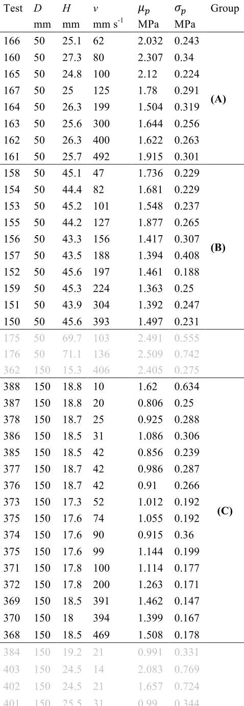
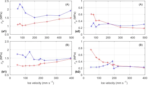
6 To show the ice velocity effect on the ice force level, four groups of data, (C), (E), (F) and (J) at different 1

structural widths with similar ice thickness are selected from Table 1, as shown in Figure 1. Figure 1 (a) and 2

(b) show the mean 𝜇( and standard deviation 𝜎( of the effective pressure from the Table 1, respectively.

3

Figure 1 (c) and (d) are the maximum and minimum effective pressure calculated from 𝜇₍± 2𝜎₍, respectively. 4

In Figure 1 (a) and (c), the pressure decreases from higher value to the lowest value first before ice velocity 5

reaches the transition ice velocity. Reason of this pressure difference can be the difference between static 6

frictional force at low velocity and kinetic frictional force at high velocity (Ji and Oterkus, 2018). After the 7

transition ice velocity, the mean value increases approximately linearly with increasing ice velocity. It is due 8

to the fact that there is more momentum energy transferred to the structure from ice, i.e. higher acceleration 9

of the structure in the form of 𝐹 = 𝑀(𝜕𝑣/𝜕𝑇). Apart from ice speed effect, it shows that thicker ice has 10

higher effective pressure and wider structure has lower effective pressure. In other words, the higher the aspect 11

ratio of structural width D over ice thickness H, the lower the effective pressure is. 12

Figure 1 (b) shows the standard deviation of pressure decreases with increasing velocity. The decreasing trend 13

indicates smaller ice failure size and the occurrence of more non-simultaneous failure. Provided that the 14

minimum effective pressure to be 𝜇₍− 2𝜎₍, Figure 1 (d) also indicates that it has more dependency on ice 15

velocity and less dependency on structural width or ice thickness. Slope at lower velocity is higher since 16

simultaneous failure has large standard deviation caused by the maximum force value. For the same reason, 17

the data points at lower velocity calculated in this method has less accuracy. Because there should not be any 18

of negative pressure. Then the minimum value increases approximately linearly with ice velocity, which 19

means that the lower bound of ice force follows the similar pattern. Considering that most part of the ice 20

maintains constant contact with structure at high ice speed after failure, ice force will not reduce back to zero 21

as that at lower ice speed. 22

7

[image:7.595.50.545.47.432.2]

1

Fig. 1. Ice velocity vs. the (a) mean, (b) standard deviation, (c) maximum and (d) minimum of effective 2

pressure from the data group of (C), (E), (F) and (J) in Table 1. 3

3. MODEL DESCRIPTION

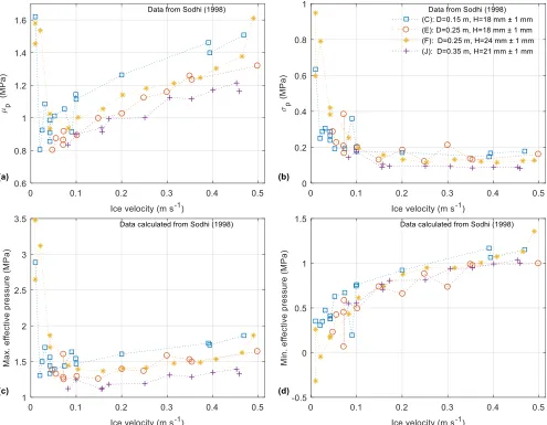
4

3.1 Ice failure zone 5

The governing equations in the model proposed here are mainly adopted from Ji and Oterkus (2018). There 6

are some improvements between the previous work and the current one. The previous ice failure length, 7

0 0

2 ( / )( / )

L= H v v K K , in the single ice strip model with different structural rigidities and ice velocities were 8

justified in Ji and Oterkus (2018). The constant of 2, as Sodhi used, was in the range of 1-3 in the experiment. 9

Therefore, 𝑐 is assumed to follow a normal relationship in the range of 1-3. As shown in Figure 2, the ice 10

sheet is modeled as multiple strips moving towards a mass-spring-damper idealized structure. Each ice strip 11

is assumed to be independent of each other and fails at a normally distributed random length of L_i, as 12

specified in Eq. (1) 13

0 0

( / )( / )

i

L =cH v v K K (1)

14

where Li is the ice failure length of each strip, c is a variable distributed normally in the form of

15

2

~ ( , _s)

c N µ σ with mean µ and variance 2

s

σ , v₀ is the reference velocity, v is the ice velocity, K₀ is 16

8 As shown in the Figure 1 (b), the decreasing standard deviation is related with the decreasing size of ice failure 1

zone. Therefore, it is presumed that ice sheet fails at smaller ice failure zones with higher ice speed with the 2

dimension of L W H_i× ×_i , as illustrated in Figure 1, where the width of an ice failure zone 𝑊₇ is equal to the 3

structural width D over the number of ice strips, i.e. 𝑊₇ = 𝐷/𝑁_:;<7(. Besides a decreasing ice failure length 4

with increasing ice speed relationship, the width 𝑊₇ is also assumed to be inversely proportional to the ice 5

velocityv. In other words, the number of ice strips 𝑁_:;<7( is proportional to ice velocity v, as specified in 6

Eq. (2), which means that there are more ice strip failure across the interaction surface as the ice speed 7

increases, 8

eg

(20 1)

strip s

N = v+ N (2)

9

where 𝑁_:=> is the corresponding number of segments in Sodhi’s experiment and each segment has a width 10

of 50 mm, i.e. 𝑁_:=>= 1, 3, 5, 7 at 𝐷= 50, 150, 250 ,350 mm, respectively. The constant 20 is calibrated based 11

on the comparison between numerical and experimental results and the 𝑁:;<7( should be round up to an

12

integer during calculation in the case of a decimal value. 13

[image:8.595.90.509.283.522.2]

14

Fig. 2. Schematic sketch of non-simultaneous dynamic ice-structure model. 15

3.2 Governing equations 16

In this study, compared with the model in Ji and Oterkus (2018), the ice sheet is extended to multiple strips 17

for non-simultaneous failure characteristics in Eq. (3) and (4). Each ice failure zone applies a local ice force 18

to the structure that is controlled by the product of area and stress and the variable q_i from Van der Pol 19

oscillator equation adjusted by a magnification factor A. By adding up each local ice force, the total ice force 20

will result in the structure to vibrate in a single degree-of-freedom first-mode motion. The Van der Pol equation 21

is an oscillator with non-linear damping to describe the saw-tooth ice force fluctuation characteristic. There 22

are internal and external effects regarding the oscillator in Eq. (4). Internal effect is an assumption that ice has 23

its own original failure characteristic length which corresponds to the oscillator without relative velocity 24

related forcing term on the right-hand side of the oscillator equation. By considering internal effect only, the 25

ice failure frequency can be calculated using the relationship

f v L

_i

=

/

_i. External effect corresponds to structural 26

Ice failure zone

9 effects including structural displacement and structural velocity, i.e. relative displacement and relative velocity 1

between ice and structure. Relative velocity takes effect in the forcing term of the Van der Pol oscillator and 2

ice strain rate-stress function in Eq. (6). Relative displacement reflects to compressive stress resulting in ice 3

deformation and when the deformation exceeds the ice failure length L_i, ice failure occurs. Therefore, each 4

ice failure zone will fail under both internal and external effects. 5 1 ( ) strip N i i i

MX CX KX AHWσ q a =

+ + =

∑

+ (3)

6

2 2

( 1) i ( )

i i i i i i i B

q q q q Y X

H

ω

εω

ω

+ − + = − (4)

7

In Eq. (3) and Eq. (4), M is the mass of the structure, X is the displacement of the structure, the “dot” 8

symbol represents the derivative with respect to time T , C is the damping coefficient, A is the 9

magnification factor for oscillator variable adjusted from experimental data, H is the ice thickness, σ is 10

the variable ice stress satisfying Eq. (6), N_strip is the number of ice strips, qi is the dimensionless fluctuation

11

variable of each ice strip, 𝑎 and 𝜀 are scalar parameters that control the lower bound of ice force value and 12

saw-tooth ice force profile, respectively. Since Figure 1 (d) shows that the minimum effective pressure 13

increases with increasing velocity, the lower bound a is assumed to increase linearly with ice velocity, as 14

specified in Eq. (5), where the coefficients are calibrated based on the comparison between numerical and 15

experimental results for Test. 582, 576, 764 and 763. 16

( ) 7 4 / 3

a v = v+ (5)

17

2 i fi

ω

=

π

is the angular frequency of each ice strip force at each particular ice failure length, fi =v L/ i is

18

the frequency of each ice strip force, B is a coefficient depending on ice properties and Y_i is the 19

displacement of each ice strip. In conjunction with the ice stress power functions (Huang and Liu, 2009), 20

max

max

( )( / ) , / 1 ( )( / ) , / 1

d r t d r t

b r t b r t

v v v v v v v v

α

β

σ σ σ

σ

σ σ σ

⎧ − + ≤

⎪

=⎨

− + >

⎪⎩ (6)

21

where

σ

_max is the maximum stress at ductile-brittle range,

σ

_d and

σ

_b are the minimum stress at ductile 22

and maximum stress at brittle range, respectively, α and β are positive and negative indices to control the 23

envelope profile, respectively, and v_t is the transition ice velocity approximately in the middle of transition 24

range. Further and justification of the parameters are provided in detail in the next section. 25

3.3 Parameter values 26

The parameters in Eq. (1-4) and Eq. (6) are determined and calibrated by the experimental results summarized 27

in Sodhi (1998). The mass of the structure M =600 kg and damping ratio ξ =0.1 are found in the earlier 28

experimental configuration in Sodhi (1991). Ice velocity, ice thickness, structural stiffness and structural width 29

are directly used from the Table 1. Values of A, a,

ε

and B are used directly from Ji and Oterkus (2018). 30

0

K , α and β are adjusted by the preliminary simulation results from Test. 582 and Test. 576. Stress 31

variations range is approximately from 1.6 MPa to 4.5 MPa and there is a clear boundary between higher and 32

lower stress value at the velocity of 0.03 m s-1_{. Therefore, 0.03 m s} 1

t

v ₌ − _,

min 1600 kPa

σ

= and

33

max 4500 KPa

σ

= are used for the minimum and maximum stress, respectively. As suggested in Sodhi (1998), 34

1 0 0.03 m s

v = − and c varies between 1 to 3. Therefore, the mean value is set to

µ

=2 and standard 35

deviation is

σ

s =0.3. A summary of parameter values is listed below:

10 1 1 max 1 1 0 0

600 kg, 0.1, 35000 kN m 0.19, 4.6, B 0.1;

2000 kPa, 1600 kPa, 4500 kPa, 0.5, 0.7, 0.03 m s ; 0.03 m s , 10000 kN m , 2, 0.3.

d b t

s

M K A

v

v K

ξ ε

σ σ σ α β

µ σ − − − − = = = = = = = = = = =− = = = = = ， 1

4. RESULTS AND DISCUSSION 2

Based on the experimental results summarized in Table 1, four different tests, Test. 582, 576, 764 and 763, are 3

considered. To differentiate the number of numerical simulation and the experimental test, the reproduced 4

numerical results from the corresponding tests are named after STest. and with the corresponding test number, 5

i.e. numerical simulation STest. 582 for experimental Test. 582. Results obtained from the current numerical 6

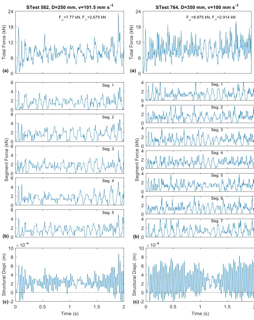
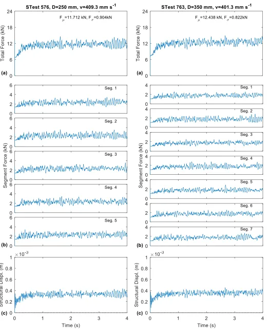
model are shown in Figures 3-6. Each figure contains time history plot of total ice force, ice force on each 7

segment and structural displacement. Comparison between numerical results and experiments shows 8

quantitively agreement with the envelope profile of all forces and structural displacement. The mean value 𝐹_%

9

and standard deviation 𝐹& of ice force are listed in Table 2, in which the force is calculated by the product of

10

interaction area and effective pressure. The difference between the results from the model and experiment for 11

[image:10.595.101.493.337.439.2]

𝐹_% and 𝐹_&, i.e. ΔF_µ and ΔF_σ, are also listed to show the error rate of results. 12

Table 2. Results from experimental tests and numerical simulations. 13

No. Test. STest. ∆𝐹% ∆𝐹&

𝐹_% (kN) 𝐹_& (kN) 𝐹% (kN) 𝐹& (kN)

582 7.856 2.354 7.77 2.675 -1.10% 13.62%

576 11.721 1.093 11.712 0.904 -0.08% -17.31% 764 8.952 3.008 8.875 2.914 -0.86% -3.11% 763 12.982 0.970 12.438 0.822 -4.19% -15.28% 14

Although force records in Figure 3 and 4 are showing non-simultaneous characteristic in general, there are 15

still different levels of simultaneousness if only one cycle of failure is considered. Force records in STest. 582 16

show that there is occurrence of a sudden peak force on all segments simultaneously, resulting in large 17

amplitude of force upon the structure, whereas peak force occurs randomly in STest. 764 upon different 18

segments of the structure. 19

The pattern of smaller variations and higher mean value of ice force with increasing ice velocity coincide with 20

the test results, as shown in Figure 3 and 5 as well as Figure 4 and 6. However, as Sodhi mentioned, variations 21

of ice force should decrease when structural width becomes larger, as in STest. 576 and STest.763 shown in 22

Figure 5 and 6, respectively. On the contrary, both numerical and test results from Test. 764 and STest.764 23

have higher standard deviation than that from Test. 582 and STest. 582. The reason is that figures in Sodhi 24

(1998) are just plotted in one second. Moreover, the starting and ending time in those figures are not picked 25

at the same time period which makes the statistics less accurate. Because of the randomness in the numerical 26

model, the occurrence and quantity of those four typical ice forces would appear randomly at both STest. 582 27

and STest. 764. This means that the randomness would exist in the real experiment. 28

Moreover, it can be noticed that there is more non-simultaneous failure in STest. 764 (Figure 4) than that in 29

STest. 582 (Figure 3) and in STest. 763 (Figure 6) than STest. 576 (Figure 5), respectively. Due to increasing 30

ice speed and structural width, the size of ice failure zone becomes smaller, i.e. the number of ice failure zone 31

increases. Hence, the possibility of non-simultaneous failure increases and variation of ice force decreases. 32

11 modes at different speeds. As the size of ice failure zone decreases with increasing ice speed, ice will fail from 1

larger size to smaller size, which corresponds to the ductile bending mode to brittle crushing mode, 2

respectively. Technically, a cycle of simultaneous ice failure will reduce back to zero value entirely after the 3

unloading phase. There are two reasons of this lower bound of ice force variations. One is attributed to the 4

non-simultaneous characteristic where there are some ice zones remaining in contact with the structure before 5

failure occurs. The other is purely physical contact with the structure leading to high level of ice force. 6

12

1

2

3 4

[image:12.595.38.552.33.680.2]

Fig. 3. Time history of (a) total ice force; (b) ice force on each segment; (c) structural displacement with 5 segments at 𝐷= 250 mm, 𝑣= 101.5 .m s-1.

Fig. 4. Time history of (a) total ice force; (b) ice force on each segment; (c) structural displacement with 7 segments at 𝐷= 350 mm, 𝑣= 100 mm s-1.

13

1

2

[image:13.595.41.567.34.678.2]

3

Fig. 5. Time history of (a) total ice force; (b) ice force on each segment; (c) structural displacement with 5 segments at 𝐷= 250 mm, 𝑣= 409.3 mm s-1.

Fig. 6. Time history of (a) total ice force; (b) ice force on each segment; (c) structural displacement with 7 segments at 𝐷= 350 mm, 𝑣= 401.3 mm s-1.

14

5. DEMOSTRATION CASES

1 2

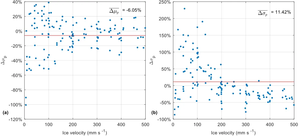
To test the calibrated model’s capability at different 𝐷, 𝐻 and 𝑣, it is used to simulate 134 different tests 3

from Group (A) to (K) in Table 1. Same configurations as those in the previous four simulations are used by 4

only changing the 𝐷, 𝐻 and 𝑣. Figure 7 (a-k) show a series of comparisons of 𝜇₍ and 𝜎₍ between the 5

model (plotted in red) and experiment (plotted in blue) as the ice velocity increases. The model captures the 6

general trend of 𝜇( and 𝜎( as v increases, especially at some fluctuation points. Meanwhile, there are

7

some abnormal experimental results that require a double-check, such as the peak points in Figure 7 g(1) and 8

h(2). The 𝜇₍ and 𝜎₍ has better accuracy as the ice velocity increases, as shown in Figure 8. The difference 9

between the results from model and experiment for 𝜇₍ and 𝜎₍, i.e. ∆𝜇₍ and ∆𝜎₍, are plotted against v

10

with the mean of -6.05% and 11.42% difference, respectively. 11

Figure 9 shows the histogram of the ∆𝜇( and ∆𝜎( with an interval of 10% between each bar. The number

12

on the top of each bar shows the corresponding percentage weighted among all data. The model can predict 13

well on the mean value that 76.8% of data yields a value within the 20% of difference between the model and 14

experiment. In terms of 𝜎₍, 71% of data yields a value within the 50% of difference and 30.7% of data yields 15

a value within the 20% of difference. The less accuracy at lower velocity range can be the reason of 16

corresponding ductile ice failure property. The failure mechanism in the numerical model is supposed to 17

simulate the crushing brittle ice failure behavior, in which ice fails at certain amount of length. 18

19

[image:14.595.43.554.332.624.2]

15

1

[image:15.595.44.551.47.336.2]

16

1

[image:16.595.43.554.51.625.2]

17

[image:17.595.44.554.46.341.2]

1

Fig. 7. Ice velocity vs. the mean 𝜇₍ and standard deviation 𝜎₍ of the effective pressure across the interaction 2

surface from numerical simulations (red line) and experimental results (blue line), at (a-b) D=50 mm, (c-d) D

3

=150 mm, (e-i) D =250 mm, (j-k) D =350 mm with the corresponding data group of (A) to (K) from Table 1. 4

5

6

Fig. 8. Ice velocity vs. (a) mean and (b) standard deviation of the effective pressure difference (in percentage) 7

between numerical simulations and experimental results. 8

[image:17.595.47.552.422.652.2]

18

[image:18.595.44.550.49.385.2]

1

Fig. 9. Histogram of (a) mean and (b) standard deviation of the effective pressure difference (in decimal) 2

between numerical simulations and experimental results. 3

6. CONCLUSION

4

To simulate non-simultaneous ice failure effects on ice-structure interaction, an extended model based on the 5

previous work of Ji and Oterkus (2018) was developed. An assumption was made that the size of ice failure 6

zone will decrease when ice velocity increases. Therefore, the ice failure length and width decreases, which 7

increase the possibility of non-simultaneous effect on ice failure. Numerical results agree well with those in 8

Sodhi (1998) and indicates that variations of ice force decrease with increasing ice velocity and increasing 9

structural width, respectively. There is simultaneous failure occurrence on all segments at lower ice velocity, 10

indicating large size of ice failure zone at ductile bending failure mode. At higher ice velocity, there is more 11

random peak forces taking place on different segments, indicating more non-simultaneous ice failures at 12

smaller brittle crushing zones. The simulation results from a series of 134 blind tests demonstrate the model’s 13

capability of predicting at different ice velocities, structural widths and ice thicknesses. In addition, analysis 14

of the ice indentation experiments shows that the mean and minimum effective pressure have an approximately 15

linear relationship with ice velocity which testified the assumption on variations of ice failure zone in the 16

model. 17

ACKNOWLEDGEMENT 18

19 of Glasgow and the University of Strathclyde for his visit to the University of Michigan.

1

REFERENCES 2

Ashby, M., Palmer, A., Thouless, M., Goodman, D., Howard, M., Hallam, S., Murrell, S., Jones, N., Sanderson, 3

T., Ponter, A., 1986. Nonsimultaneous failure and ice loads on arctic structures, Offshore Technology 4

Conference. Offshore Technology Conference. 5

Bhat, S., 1990. Modeling of size effect in ice mechanics using fractal concepts. Journal of Offshore Mechanics 6

and Arctic Engineering 112 (4), 370-376. 7

Hendrikse, H., Kuiper, G., Metrikine, A., 2011. Ice induced vibrations of flexible offshore structures: the effect 8

of load randomness, high ice velocities and higher structural modes, 21st International Conference on Port 9

and Ocean Engineering Under Arctic Conditions, p. 031. 10

Huang, G., Liu, P., 2009. A dynamic model for ice-induced vibration of structures. Journal of Offshore 11

Mechanics and Arctic Engineering 131 (1), 011501. 12

Ji, X., Oterkus, E., 2016. A dynamic ice-structure interaction model for ice-induced vibrations by using van 13

der pol equation. Ocean Engineering 128, 147-152. 14

Ji, X., Oterkus, E., 2018. Physical mechanism of ice/structure interaction. Journal of Glaciology 64 (244), 15

197-207. 16

Johnston, M., Croasdale, K.R., Jordaan, I.J., 1998. Localized pressures during ice–structure interaction: 17

relevance to design criteria. Cold Regions Science and Technology 27 (2), 105-117. 18

Karr, D.G., Troesch, A.W., Wingate, W.C., 1993. Nonlinear dynamic response of a simple ice-structure 19

interaction model. Journal of Offshore Mechanics and Arctic Engineering 115 (4), 246-252. 20

Kry, P., 1978. A Statistical Prediction of Effective Ice Crushing Stresses on Wide Structure, Proc. of IAHR Ice 21

Symposium. 22

Kry, P., 1980. Third Canadian geotechnical colloquium: Ice forces on wide structures. Canadian Geotechnical 23

Journal 17 (1), 97-113. 24

Matlock, H., Dawkins, W.P., Panak, J.J., 1971. Analytical model for ice-structure interaction. Journal of the 25

Engineering Mechanics Division 97 (4), 1083-1092. 26

Sodhi, D.S., 1991. Ice-structure interaction during indentation tests, in: Jones S., T.J., McKenna R.F., Jordaan 27

I.J. (Ed.), Ice-Structure Interaction. Springer, Berlin, Heidelberg, pp. 619-640. 28

Sodhi, D.S., 1998. Nonsimultaneous crushing during edge indentation of freshwater ice sheets. Cold Regions 29

Science and Technology 27 (3), 179-195. 30

Sodhi, D.S., Haehnel, R.B., 2003. Crushing ice forces on structures. Journal of Cold Regions Engineering 17 31

(4), 153-170. 32

Wang, L., Xu, J., 1991. Description of dynamic ice-structure interaction and the ice force oscillator model, 11 33

th International Conference on Port and Ocean Engineering under Arctic Conditions, St. John's, Canada, pp. 34

141-154. 35

Withalm, M., Hoffmann, N., 2010. Simulation of full-scale ice–structure-interaction by an extended Matlock-36

model. Cold Regions Science and Technology 60 (2), 130-136. 37

Yu, B., Karr, D., 2014. An ice-structure interaction model for non-simultaneous ice failure, OTC Arctic 38

Technology Conference. Offshore Technology Conference, p. 24547. 39

Yue, Q., Guo, F., Kärnä, T., 2009. Dynamic ice forces of slender vertical structures due to ice crushing. Cold 40

Regions Science and Technology 56 (2), 77-83. 41