University of Pennsylvania
ScholarlyCommons
Publicly Accessible Penn Dissertations
1-1-2012
Statistical Methods for Non-Ignorable Missing
Data With Applications to Quality-of-Life Data.
Kaijun Liao
University of Pennsylvania, [email protected]
Follow this and additional works at:
http://repository.upenn.edu/edissertations
Part of the
Biostatistics Commons
This paper is posted at ScholarlyCommons.http://repository.upenn.edu/edissertations/658
Recommended Citation
Liao, Kaijun, "Statistical Methods for Non-Ignorable Missing Data With Applications to Quality-of-Life Data." (2012).Publicly Accessible Penn Dissertations. 658.
Statistical Methods for Non-Ignorable Missing Data With Applications to
Quality-of-Life Data.
Abstract
Researchers increasingly use more and more survey studies, and design medical studies to better understand the relationships of patients, physicians, their health care system utilization, and their decision making processes in disease prevention and management. Longitudinal data is widely used to capture trends occurring over time. Each subject is observed as time progresses, but a common problem is that repeated measurements are not fully observed due to missing response or loss to follow up. An individual can move in and out of the observed data set during a study, giving rise to a large class of distinct "non-monotone" missingness patterns. In such medical studies, sample sizes are often limited due to restrictions on disease type, study design and medical information availability. Small sample sizes with large proportions of missing information are problematic for researchers trying to understand the experience of the total population. The information in the data collected may produce biased estimators if, for example, the patients who don't respond have worse outcomes, or the patients who answered "unknown" are those without access to medical or non-medical information or care. Data modeled without considering this missing information may cause biased results.
A first-order Markov dependence structure is a natural data structure to model the tendency of changes. In my first project, we developed a Markov transition model using a full-likelihood based algorithm to provide robust estimation accounting for "non-ignorable'' missingness information, and applied it to data from the Penn Center of Excellence in Cancer Communication Research. In my second project, we extended the method to a pseudo-likelihood based approach by considering only pairs of adjacent observations to significantly ease the computational complexities of the full-likelihood based method proposed in the first project. In my third project, we proposed a two stage pseudo hidden Markov model to analyze the association between quality of life measurements and cancer treatments from a randomized phase III trial (RTOG 9402) in brain cancer patients. By incorporating selection models and shared parameter models with a hidden Markov model, this approach provides targeted identification of treatment effects.
Degree Type
Dissertation
Degree Name
Doctor of Philosophy (PhD)
Graduate Group
Epidemiology & Biostatistics
First Advisor
Keywords
Clinical trial /Cancer applications, Composite likelihood /pseudo likelihood method, Conjoint analysis, Hidden Markov model, Longitudinal and multivariate data, Non-ignorable missing data
Subject Categories
STATISTICAL METHODS FOR NON-IGNORABLE MISSING DATA WITH
APPLICATIONS TO QUALITY-OF-LIFE DATA.
Kaijun Liao
A DISSERTATION
in
Epidemiology and Biostatistics
Presented to the Faculties of the University of Pennsylvania
in
Partial Fulfillment of the Requirements for the
Degree of Doctor of Philosophy
2012
Supervisor of Dissertation
Andrea B. Troxel, Professor of Biostatistics
Graduate Group Chairperson
Daniel F. Heitjan, Professor of Biostatistics
Dissertation Committee
Mary E. Putt, Associate Professor of Biostatistics
Benjamin C. French, Assistant Professor of Biostatistics
STATISTICAL METHODS FOR NON-IGNORABLE MISSING DATA WITH
APPLICATIONS TO QUALITY-OF-LIFE DATA.
c
COPYRIGHT
2012
Kaijun Liao
This work is licensed under the
Creative Commons Attribution
NonCommercial-ShareAlike 3.0
License
To view a copy of this license, visit
ACKNOWLEDGEMENT
Completing a PhD is truly like running a marathon, and I would not have been able to
complete this journey without the support of many people. I must first express my gratitude
to my advisor, Prof. Andrea B. Troxel, as an outstanding advisor and excellent professor.
She provided me many insightful comments and advice, constant encouragement, and
in-valuable suggestions which guided me through all the challenges and difficulties during the
entire process of completing my doctoral work. What’s most important is that she taught
me how to be an excellent statistician and this experience will definitely benefit me for
my entire career. I would like to thank all the members of my committee, Prof. Katrina
Armstrong, Prof. Mary E. Putt, and Prof. Benjamin C. French, for their insightful
com-ments, and their time and effort in reviewing and improving the quality of this work. I also
feel lucky to have the opportunity to work with Prof. Katrina Armstrong’s research team
and collaborate on many levels of the research projects. I highly appreciate her knowledge,
expertise, understanding, and patience, which added considerably to my graduate
experi-ence. I would like to thank Prof. Mary E. Putt for advising my master level project and
all her encouragement, Prof. Nandita Mitra for her career suggestions and class selection
during the graduate years, Prof. Benjamin C. French for reviewing my thesis and providing
valuable feedback, and other faculty members at Penn who have offered me tremendous
help throughout my Ph.D. years.
Finally, I am deeply and forever indebted to my parents and my wife for their love,
sup-port and encouragement throughout my entire life. Without their love and supsup-port, this
ABSTRACT
STATISTICAL METHODS FOR NON-IGNORABLE MISSING DATA WITH
APPLICATIONS TO QUALITY-OF-LIFE DATA.
Kaijun Liao
Andrea B. Troxel
Researchers increasingly use more and more survey studies, and design medical studies
to better understand the relationships of patients, physicians, their health care system
utilization, and their decision making processes in disease prevention and management.
Longitudinal data is widely used to capture trends occurring over time. Each subject is
observed as time progresses, but a common problem is that repeated measurements are not
fully observed due to missing response or loss to follow up. An individual can move in and
out of the observed data set during a study, giving rise to a large class of distinct
“non-monotone” missingness patterns. In such medical studies, sample sizes are often limited
due to restrictions on disease type, study design and medical information availability. Small
sample sizes with large proportions of missing information are problematic for researchers
trying to understand the experience of the total population. The information in the data
collected may produce biased estimators if, for example, the patients who don’t respond
have worse outcomes, or the patients who answered “unknown” are those without access to
medical or non-medical information or care. Data modeled without considering this missing
information may cause biased results.
A first-order Markov dependence structure is a natural data structure to model the tendency
of changes. In my first project, we developed a Markov transition model using a
full-likelihood based algorithm to provide robust estimation accounting for “non-ignorable”
missingness information, and applied it to data from the Penn Center of Excellence in Cancer
pseudo-likelihood based approach by considering only pairs of adjacent observations to significantly
ease the computational complexities of the full-likelihood based method proposed in the
first project. In my third project, we proposed a two stage pseudo hidden Markov model to
analyze the association between quality of life measurements and cancer treatments from
a randomized phase III trial (RTOG 9402) in brain cancer patients. By incorporating
selection models and shared parameter models with a hidden Markov model, this approach
TABLE OF CONTENTS
ACKNOWLEDGEMENT . . . iii
ABSTRACT . . . iv
LIST OF TABLES . . . ix
LIST OF ILLUSTRATIONS . . . x
CHAPTER 1 : Introduction . . . 1
CHAPTER 2 : A transition model for quality of life data with ignorable non-monotone missing data . . . 6
2.1 Introduction . . . 6
2.2 Methods and Notation . . . 11
2.3 Example: Analysis of PCIE Data . . . 16
2.4 Simulation Study . . . 19
2.5 Discussion . . . 23
CHAPTER 3 : Pseudo-likelihood methods for transition models in longitudinal data with non-ignorable non-monotone missing data . . . 30
3.1 Introduction . . . 30
3.2 Model and Notation . . . 34
3.3 Example: Analysis of PCIE Data . . . 41
3.4 Simulation Study . . . 45
3.5 Discussion . . . 48
4.1 Introduction . . . 56
4.2 Motivating Example . . . 58
4.3 Methods and Notation . . . 61
4.4 Simulation Study . . . 74
4.5 Example: Analysis of RTOG Data . . . 78
4.6 Discussion . . . 88
CHAPTER 5 : Conclusion . . . 100
APPENDIX . . . 102
LIST OF TABLES
TABLE 2.1 : Missingness patterns in PCIE study . . . 24
TABLE 2.2 : Response rate for possible outcome . . . 24
TABLE 2.3 : Characteristics of covariates . . . 25
TABLE 2.4 : Pearson correlation matrix of exercise score . . . 25
TABLE 2.5 : Longitudinal analysis of PCIE data . . . 26
TABLE 2.6 : Simulation study 500 replicates . . . 27
TABLE 2.7 : Model comparison simulations, 1000 replicates . . . 28
TABLE 2.8 : Simulation comparison study, 500 replicates . . . 28
TABLE 2.9 : Non-normal data, 500 replicates . . . 29
TABLE 3.1 : Missingness patterns in PCIE study . . . 50
TABLE 3.2 : Response rates for possible outcomes . . . 50
TABLE 3.3 : Patient characteristics by response time . . . 50
TABLE 3.4 : Longitudinal analysis of PCIE data . . . 51
TABLE 3.5 : Simulation study of sensitivity to sample size, 1000 replicates . . . 52
TABLE 3.6 : Simulation study of model comparison, 500 replicates . . . 53
TABLE 3.7 : Simulation study of sensitivity to different covariance structures, 1000 replicates . . . 54
TABLE 3.8 : Simulation study of normal data vs gamma data, 500 replicates . . 55
TABLE 4.1 : Patients characteristics by arm . . . 90
TABLE 4.2 : Simulation of model comparisonn= 150: SHMM vs SPHMM . . . 91
TABLE 4.3 : Simulation of model comparisonn= 300: SHMM vs SPHMM . . . 92
TABLE 4.4 : Simulation of sensitivity analysis: transition matrixQA . . . 93
TABLE 4.5 : Simulation of sensitivity analysis: transition matrixQB . . . 94
TABLE 4.7 : Analysis for 5 years data: B-QLQ . . . 96
TABLE 4.8 : Patients characteristics by arm for at least 2 years survival . . . 97
TABLE 4.9 : Data analysis for at least 2 years survival: MMSE . . . 98
LIST OF ILLUSTRATIONS
FIGURE 4.1 : MMSE response rate for 5 years follow up. . . 81
FIGURE 4.2 : B-QLQ response rate for 5 years follow up. . . 81
FIGURE 4.3 : MMSE: response rate for at least 2 years survival. . . 84
CHAPTER 1 : Introduction
In chronic disease studies, questionnaires are an often primary source of information to
measure changes in attitude or compliance with treatment or medical advice. More and
more survey studies focus on questionnaires of patients with different health issues, stages of
disease, types of cancer, and other medical/non-medical information so that health providers
or decision makers can better understand patient behavior and the estimates of treatment
effects. The underlying structure of the quality and quantity of information that can be
collected from each participant can be complicated due to the fact that during follow-up,
the occurrence of observations at a given time depends on many observed or unobserved
factors. Intuitively, patient behavior involves attitudes and knowledge. So questionnaires,
health-related attitudes and information clearly are relevant. It is reasonable to expect that
patients’ responses could be lower for those with worse health, or could be a function of
all health information, such as disease type, how actively patients seek medical help, and
their supporting environment; this makes the missingness more likely to be informative.
Longitudinal data is widely used to monitor disease progression, or investigate changes over
time in a characteristic which is measured repeatedly for each study participant. Missing
information is typically inevitable in longitudinal studies, and can result in biased estimates
and a loss of power when the missingness is informative.
In Chapter 2, we propose a full-likelihood based transition model and apply it to data from
the Penn Center of Excellence in Cancer Communication Research, a cancer-related survey
study recently conducted at the University of Pennsylvania. One of the research goals of
the study was to examine how the Patient-Clinician Information Engagement (PCIE) score
affects cancer patients’ attitudes and behaviors in breast, prostate, and colorectal cancers;
in particular, researchers were interested in the amount of exercise the patients were engaged
in. Decisions people choose to follow will impact their health status. For example, patients
decide whether to increase exercise, to get radiation therapy, or to choose surgery after
be influenced by both medical and non-medical information. A random sample was selected
in fall 2006 from the Pennsylvania Cancer Registry (PCR). Patients had to have one of the
above three cancers, diagnosed in 2005. There were a total of 2010 cancer patients who
responded to at least one of three surveys, including 650 patients with prostate cancer, 682
patients with colorectal cancer, and 678 patients with breast cancer. The study included
three longitudinal surveys. Surveys were initially conducted in fall 2006, with the second
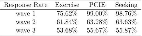
and third waves conducted in fall 2007 and fall 2008. The response rate for PCIE scores
were 99.00% for wave one, 63.28% for wave two, and 55.67% for wave three. Clearly this
study resulted in a large amount of missing data for unknown reasons, and thus requires
careful attention to the issue of missingness.
We use a full-likelihood based method to analyze continuous longitudinal responses with
non-ignorable non-monotone missing data, and consider a transition probability model for
the missingness mechanism. A first-order Markov dependence structure is assumed for
both the missingness mechanism and observed data. This process fits the natural data
structure in the longitudinal framework. Instead of using logistic regression to model the
missing mechanism, we propose a beta-binomial distribution to model the probability of
non-response. The beta-binomial distribution can be extended to the multivariate Polya
distribution when there are more than two types of responses; our main interest is in
esti-mating the parameters of the marginal model and evaluating the MAR (missing at random)
assumption in the Effects of Public Information Study. We also present a simulation study
to assess model performance in small samples, addressing the basic issues of bias in the
parameter estimates and computing coverage probabilities, while varying the covariance
structure of the longitudinal outcomes. The marginal effects are estimated well even when
the underlying data distribution is not normal. However, full-likelihood based methods
require integration over the unobserved data. The parameter estimation has to be done
numerically, and this can be computationally prohibitive due to the complicated joint
Pseudo-likelihood methods (Gong and Samaniego, 1981; Parke, 1986) and composite marginal
likelihood methods (Cox and Reid, 2004; Varin et al., 2011) are widely used to ease the
com-putational complexities of the conventional likelihood-based method. The pseudo-likelihood
methods can be viewed as an extension of composite marginal likelihood methods, which can
be transferred into the non-ignorable non-monotone missing data framework. In Chapter
3, we propose a pseudo-likelihood method based on the conditional density of all adjacent
pairs of assessments, with a first-order auto-regressive covariance structure to account for
the correlation of the repeated observations within subjects. Estimation proceeds using
the score vector, which guarantees a consistent estimator. Although the
pseudo-likelihood method achieves asymptotically unbiased estimators of the regression
parame-ters and missingness parameparame-ters if the model is correctly specified, these estimators can be
highly inefficient in the case of faulty assumptions about the covariance structure across
measurement times. A sandwich estimator is used to obtain correct inference for variance
parameters. We fitted the proposed method to the same data from the Penn Center of
Excellence in Cancer Communication Research as in project one. A simulation study
in-vestigates the empirical behavior of the proposed models, compared to the full-likelihood
method proposed in Chapter 2. The simulation study shows that this approach can handle
longitudinal data with various covariance structures well and is no more computationally
intensive than the independent pseudo-likelihood model (Troxel et al., 1998b). This
ap-proach can handle a mis-specified correlation to some extent. In simulation studies with
a variety of mis-specified correlation structures, the marginal effects and missingness
ef-fects consistently have high coverage probabilities as long as the correlation among pairs is
nonzero.
In Chapter 4, we extend our approach using a hidden Markov model framework. By
incorporating both selection models and shared parameter models, we can identify
dif-ferences among the transition processes with incomplete data simultaneously in both a
state-dependent model and a missingness mechanism model. The conditional
multi-dimensional integration in traditional methods into one dimensional integration in
the observed likelihood. In addition, the proposed models avoid the problem of
specifica-tion of the correlaspecifica-tion structure of repeated outcomes by instead emphasizing estimaspecifica-tion
in Markov Chain parameters. We propose a generalized linear model and generalized
lin-ear mixed model framework, using a Baum-Welch algorithm (Baum et al., 1970; Rabiner,
1989; Welch, 2003) to update the Markov Chain parameters to provide efficient
parame-ter estimation in the general situation of non-ignorable non-monotone longitudinal missing
data. A two-stage pseudo-likelihood method is used to reduce the parameter space to make
this model more attractive. Our proposed method is applied to data from a randomized
phase III intergroup trial conducted by the Radiation Therapy Oncology Group (RTOG
9402) between 1994 and 2002, coordinated by the National Cancer Institute, in anaplastic
oligodendroglioma (AO) brain tumor, patients received either chemotherapy plus radiation
therapy (Arm 1) or radiation therapy alone (Arm 2), as previously described by Cairncross
et al. (2006) and Wang et al. (2010). Previous reports had shown that AO patients
re-spond to surgery and radiotherapy (RT) at diagnosis, as well as to procarbazine, lomustine,
and vincristine (PCV) chemotherapy; it was unclear whether patients would benefit from
combined PCV and RT therapy, compared to RT alone. Study reports also showed that
patients who lack the 1p and 19q chromosomes have significantly longer progression
sur-vival times when treated with PCV+RT, but this is associated with substantial toxicity. In
RTOG 9402, there was no significant difference in median survival times between the two
treatment arms in patients with only one co-deletion or no deletions of chromosomes. The
effect of toxicity and side effects from PCV chemotherapy and RT on patients’ neurologic
functioning and global quality of life remains unclear. Several measures were collected at
each visit to assess patients cognitive ability and attitudes on quality of life during the
study time period, including Karnofsky performance status (KPS), which measures
phys-ical well-being; the Mini-Mental Status Exam (MMSE), which measures cognitive ability
as assessed by a nurse, research associate, or physician to reflect the opinions of the health
mea-sures patient-reported quality of life. In this Chapter, we focus on the association between
patients’ MMSE/B-QLQ scores and treatment effect. By modeling the disease
progres-sion through different hidden states, our approach allows more precise identification of the
CHAPTER 2 : A transition model for quality of life data with non-ignorable
non-monotone missing data
2.1. Introduction
In a longitudinal study, each subject is observed as time progresses. A common problem
is that repeated measurements are not fully observed due to missing responses or loss
to follow up. An individual can move in and out of the observed data set during the
study, giving rise to a large class of distinct “non-monotone” missingness patterns. The
appropriate statistical methods differ based on the nature of the data structure and missing
mechanism. The simplest types of incomplete data are when the missingness is MCAR
(missing completely at random) or MAR (missing at random). Little and Rubin (1987)
and Allison (2001) provide helpful terminology to describe missing data mechanisms and
a comprehensive overview of methods in this setting. Most approaches can be categorized
as selection models, pattern-mixture models or shared-parameter models depending on the
factorization of the joint likelihood of the outcomes and missingness indicators. This article
will focus on selection models.
Under the MCAR mechanism, the observed data can be viewed as a random subset of
the complete data. For the MAR assumption, the missingness mechanism depends only
on observed quantities. Both mechanisms can be treated as “ignorable” if the parameters
in the two parts of the model are distinct. For “ignorable” data, generalized estimating
equations (GEE) provide asymptotic unbiased estimation if the underlying data is MCAR
(Liang and Zeger, 1986). Weighted generalized estimating equations (WGEE) can provide
unbiased estimation if the underlying data is MAR (Robins and Rotnitzky, 1995).
How-ever, none of above methods can provide consistent unbiased estimators under informative
dropout or non-ignorable missingness. The approaches to modeling informative drop out
or non-ignorable missing data in the longitudinal setting depend on the nature of the data
proposed methods assume a multivariate Gaussian distribution for the outcomes, with
dif-ferent specifications of the covariance structure; these include (Verbyla and Cullis, 1990;
Richard and Lynn, 1990; Munoz et al., 1992; Diggle and Kenward, 1994). Diggle and
Ken-ward (1994) proposed a likelihood-based method for continuous longitudinal outcomes with
non-ignorable or informative drop-out. They specified a multivariate Gaussian distribution
for the data and a logistic model for the probability of missing observations. Their model
allowed the missingness probability to depend on previous and current measurements, and
the likelihood was integrated over the range of the unobserved values. The likelihood
in-volved approximations with numerical integration and iterative computations. However,
their method required monotone missingness, also called informative drop-out.
Troxel et al. (1998a) extended the method to allow a non-monotone and non-ignorable
missingness mechanism. They proposed a logistic model that allowed the probability of
non-response to depend on the value of the current and/or previous measurement, allowing for
a non-ignorable missing data mechanism, and assumed multivariate Gaussian distribution
for the underlying outcomes. They assumed a first-order Markov dependence structure to
facilitate estimation.
Another way to attack the problem of non-ignorable non-monotone missingness in
longitu-dinal data is using pseudolikelihood methods to greatly ease the computational burdens of
the full-likelihood method, by setting the nuisance parameter at zero or some convenient
estimate. Troxel et al. (1998b), Sinha et al. (2010), and Parzen et al. (2007) used
pseudolike-lihood methods to deal with the binary case. Troxel et al. (2010) used an optimal weighted
combination of two pseudolikelihoods to increase the efficiency of the estimation. Tsonaka
et al. (2009) considered a semi-parametric shared parameter model without assuming any
parametric assumption for the random effects distribution.
Our method is an extension of the work of Troxel et al. (1998a). As in the earlier work
we adopt the multivariate Gaussian distribution assumption for the underlying data and
the missing mechanism, we propose a beta-binomial distribution to model the
probabil-ity of non-response. The multivariate Polya distribution is a high-dimensional version of
the beta-binomial distribution; the beta and binomial distributions correspond to Dirichlet
and multinomial distributions, respectively, in the multivariate situation. Because of this
property, our approach can be easily extended into more than one state of missingness,
such as intermediate missingness, drop-out or even death if there is non-response due to
death. Because of the Gamma function and/or Beta functions involved, closed-form
maxi-mum likelihood estimates are impractical. We propose to use Gauss-Hermite quadrature as
suggested in Liu and Pierce (1994) to approximate the likelihood. The
Broyden-Fletcher-Goldfarb-Shanno (BFGS) (Nocedal and Wright, 2006) algorithm is applied to search for
optimal solutions. The beta-binomial model provides superior model fitting to the data
compared to a traditional logistic model, especially for binary data with unbalanced sparse
data. From a Bayesian perspective, the beta is the conjugate prior distribution for the
parameters of the binomial distribution. The parametersα and β of the beta distribution
can be thought of as pseudo-observations of “success” and “failure” to be added to the
ac-tual number of successes or failures observed. This helps to stabilize the estimation of the
missingness mechanism, especially when some time points have small amounts of missing
or no missing data. This mixture model also reduces multimodality in the likelihood.
The proposed methods were applied to the data from the Penn Center of Excellence in
Cancer Communication Research. Effectiveness of communication between patients and
their physicians is a very important factor in cancer research, and throughout the health
care system. Effective exchange of information between patients, physicians, health care
systems, and the environment surrounding them determines how active participants are
within the health care system. There are many studies showing a link between highly
isolated areas or individuals and worse outcomes in cancer research (Putt et al., 2009),
including shorter survival time, worse quality of life, and lower rates of participation in
recommended treatment programs. The rate of patient adherence to a recommended course
treatment and quality of life from different channels (Tan et al., 2011). So it is crucial to
understand the relationship between patients, their physicians, and the health care system
around them, as well as the role of shared decision-making skills; how patients get, give,
and discuss information and make health care decisions is important in cancer research,
especially given the high demands that the healthcare system is facing.
There are a total of 2010 cancer patients who responded to at least one of three surveys,
including 650 patients with prostate cancer, 682 patients with colorectal cancer, and 678
patients with breast cancer. The study included three longitudinal surveys. Surveys were
initially conducted in fall 2006, with the second and third waves conducted in fall 2007
and fall 2008. The response rates of possible explanatory variables are listed in Table 2.2.
Clearly this study resulted in a large amount of missing data for unknown reasons, may
have an important impact on inference derived from this study.
The study sample was randomly selected in fall 2006 from the Pennsylvania Cancer Registry
(PCR). Patients had to have one of the above three cancers, diagnosed in 2005. The
American Association for Public Opinion Research (AAPOR, 2006) response rates for the
primary sample were 68%, 64%, and 61% for the respective cancer groups (Nagler et al.,
2010). Surveys were mailed to all participants using Dillman’s design method (Dillman,
2010). All patients were first mailed an introductory letter explaining the purpose of the
study and including instructions; the surveys were mailed in a subsequent packet with a
small monetary incentive ($3 or $5 for the short or long version of the survey). Reminder
letters were sent after 2 weeks for subjects who did not return the survey. Patient consent
was provided prior to participation, and the University of Pennsylvania Institutional Review
Board reviewed and approved this study.
One of the research goals of the study described here is to examine how the Patient-Clinician
Information Engagement (PCIE) score affects breast, prostate, and colorectal cancer
pa-tients’ attitudes and behaviors; in particular, researchers were interested in the amount of
status. For example patients decide whether to increase exercise, to get radiation
ther-apy, or to choose surgery after seeking treatment information from their physicians. The
decision making process may be influenced by both medical and non-medical information.
PCIE scores are measured from 8 items; for each item, patients think back to the first
few months of their cancer diagnosis and recall whether they have 1) sought information
about treatments from their treating physician; 2) sought treatment information from other
physicians or health professionals; 3) actively looked for information about their cancer from
their treating physician; 4) actively looked for information about their cancer from other
physicians or health professionals; 5) discussed information from other sources with their
treating physician; 6) received suggestions from their treating physician to get information
from other sources; 7) actively looked for information about quality of life issues from their
treating physician; and 8) looked for quality of life information from other physicians or
health professionals. Each of the eight items was transformed to a Z-score, and the average
of the eight Z-scores formed the PCIE scale.
We use the extent of exercise (“During an average week, how many days do you exercise?”)
as the primary outcome. The outcomes range from 0 to 7 by experimental design; we treat
these as continuous responses in this small interval. The Pearson correlation coefficients
in Table 2.4 suggest that the correlation between baseline and follow-up is greater than
the correlation among the follow-up assessments. We use the unstructured correlation
in the data analysis and simulation sections, and we extend the correlation into AR(1),
exchangeable and Toeplitz later in the simulation section for further model assessment.
The proposed methods are described in Section 2.2, and illustrated with an analysis of the
PCIE data in Section 2.3. A simulation study to address the performance of the methods
2.2. Methods and Notation
2.2.1. Notation and underlying assumptions
Given a longitudinal data set, let Yi = (Yi1, Yi2, . . . , YiT)
0
represent the vector of repeated
measurements for subjecti(i= 1, . . . , n) withT measurement times. LetXibe a vector ofp
covariates observed on theith subject. The covariate vectorXicould be either time
indepen-dent or time depenindepen-dent. Because the repeated measurements are not fully observed at each
time pointt= (1, . . . , T), define a vector of missingness indicatorsRi = (Ri1, Ri2, . . . , RiT)
to correspond with the outcome vector Yi= (Yi,obs,Yi,mis). Each element of Ri is defined
as
Rit =
0 if missing
1 if observed
.
For each subject, the full data are given by the repeated measurements and missingness
indicators with joint distribution L(θ, β|Yi,Ri,Xi) ∝ P(Yi,Ri|Xi, θ, β). By partitioning
Yi into (Yi,obs,Yi,mis), we can rewrite the joint likelihood in several ways. θ is parameter
space associated with outcome process, andβis parameter space associated with missingness
mechanism. A selection model would specify the joint distribution using the marginal
distribution of the repeated outcomes and the conditional distribution of missing indicators:
P(Yi,Ri|Xi, θ, β) =P(Yi,obs,Yi,mis|Xi, θ)P(Ri|Yi,obs,Yi,mis,Xi, β).
A pattern-mixture model assumes the full data have different distributions across strata
determined by the pattern of missingness:
P(Yi,Ri|Xi, θ, β) =P(Ri|Xi, β)P(Yi,obs,Yi,mis|Ri,Xi, θ).
indicators conditional on group of shared parameters γ:
P(Yi,Ri|Xi, θ, β) =
Z
P(Yi,obs,Yi,mis|γi,Xi, θ)P(Ri|γi,Xi, β)p(γi)dγi.
In our study, we focus on selection models, which are a natural way to factor the joint
likelihood function. The diagram below indicates the relationships among the variables
graphically. Each line indicates the dependence between the nodes.
Yi1 −→ Yi2 · · · Yi,T−1 −→ YiT
↓ · · · ↓ · · · ↓ · · · ↓
Ri1 −→ Ri2 · · · Ri,T−1 −→ RiT
We adopt a similar model to Troxel et al. (1998a), and assume Yi ∼M V N(µi,Σ), where
the mean structure µi = (µi1, µi2,· · ·µiT) depends on a p-dimensional covariate vector
Xi. We also assume a first-order Markov dependence structure for both the full
out-come data and the missingness indicators, so that f(Yit|Yi1, Yi2, . . . Yit−1) = f(Yit|Yit−1)
and f(Rit|Ri1, Ri2, . . . Rit−1) = f(Rit|Rit−1). Let σ2t = var(Yit) and ρt = corr(Yit, Yit+1).
Then we can denote the conditional likelihood as
Yit|Yi,t−1∼N n
µit+ρt−1 σt σt−1
(Yi,t−1−µi,t−1), σt2(1−ρ2t−1) o
.
ForT = 3 the first-order ante-dependence structure is denoted as :
Σ =
σ21 σ1σ2ρ1 σ1σ3ρ1ρ2
σ2σ1ρ1 σ22 σ2σ3ρ1
σ3σ1ρ1ρ2 σ3σ2ρ2 σ32
2.2.2. Missingness mechanism model
Unlike other approaches to modeling the missingness mechanism, we are interested in the
transition probability of the missingness indicators Rit. Conditional on each time t, the
missingness mechanism becomes a two-state Markov chain. We model the transition
prob-abilitiesπjk =P r(Rit=j|Ri,t−1 =k, Yit, Xit), j= 0,1;k= 0,1 as
π00 π01
π10 π11
which satisfy the equation π00+π01 = π10+π11 = 1. We assume that the initial state is
independent, and definenj,k as the number of times in the whole sequence thatkis followed
by j:
nj,k =PTt=1I(Rt=j|Rt−1 =k)
nj.= P
knj,k, n.k = P
jnj,k.
Then the missingness mechanism can be written as
Li =πn00i00π01ni01π10ni10π11ni11
=QT t=2
Q1 j=0
Q1
k=0πjk(t)I(Ri,t=j|Ri,t−1=k).
This becomes a product of binomial distributions. Logistic regression has been used for this
type of problem but yield unstable estimates for binary outcomes near the boundary of the
parameter space. Thus we estimate the probability of missingness at each time t using a
joint beta-binomial distribution.
Given timet−1, the missingness mechanism follows (Ri,t|Ri,t−1 =k)∼Bernoulli(πikt); we
have
f(Ri,t|Ri,t−1, yit, π) = 1 Y
k=0
πI(Rit=1)I(Rit−1=k)
k1 (1−πk1)
[1−I(Rit=1)]I(Rit−1=k)
f(πk1|ak1, bk1) =
Γ(ak1+bk1)
Γ(ak1)Γ(bk1)
×πak1−1
k1 (1−πk1) bk1−1.
Integrating the π out, the mixture function can be expressed as
f(Ri,t|Ri,t−1, aik1, bik1, yit) = Z 1
0
f(Ri,t|Ri,t−1 =k, πikt)f(πikt|aikt, bikt, yit)dπikt
=
1 Y
k=0
Γ(aik1+bik1)
Γ(aik1)Γ(bik1)
× Γ(aik1+I(Ri,t = 1)I(Ri,t−1 =k))Γ(bik1+ [1−I(Ri,t = 1)]I(Ri,t−1=k)) Γ(aik1+bik1+I(Rit−1 =k))
with aik1 = exp(ζ1Xit+ϑ1Yit +ψ1Ri,t−1) and bik1 = exp(ζ2Xit +ϑ2Yit+ψ2Ri,t−1).
However, the link function chosen could be different resulting in a different missingness
mechanism model. For givenRi,t−1 = 0, the transition probability can be denoted as
P(Rit=l|Rit−1 = 0, Yit, Xit) : =
1
1+exp((ζ1−ζ02)Xit+(ϑ1−ϑ2)Yit)
if l= 1
1 1+exp(−(ζ1−ζ
0
2)Xit−(ϑ1−ϑ2)Yit)
if l= 0
.
For givenRi,t−1= 1,
P(Rit=l|Rit−1 = 1, Yit, Xit) : =
1
1+exp((ζ1−ζ2)Xit+(ϑ1−ϑ2)Yit+(ψ1−ψ2)) if l= 1
1
1+exp(−(ζ1−ζ2)Xit−(ϑ1−ϑ2)Yit−(ψ1−ψ2)) if l= 0
.
Notice that if ϑ1 −ϑ2 6= 0 then the missingness mechanism is indeed non-ignorable since
the probability of missingness depends on the unobserved outcome Yit. In practice, only
the difference of each parameters are identifiable, not the individual parameters. We let
mechanism model, where ζc is the coefficient of the covariates, ϑc is the coefficient of the
current observationyit ,andψc is the coefficient of the previous missingness indicatorrit−1.
The link function for parameters aikt and bikt of the Beta distribution could be chosen
differently than a simple exponential function, and this will result a different
missing-ness mechanism model. The missingmissing-ness mechanism model could be expanded, similar
to Dirichlet-Multinomial distribution, from the current Beta-Binomial distributions when
modeling a missing data indicator with more than two levels, such as “observed”,
“inter-mittently missing”, “drop out”.
2.2.3. Parameter estimation
The observed joint likelihood function can be denoted as
Li(µ,Σ, θ, β) = f(Yi,obs,Ri)
=
Z . . .
Z
f(Yi,obs,Yi,miss,Ri)dYi,miss
=
Z . . .
Z
f(Yi1)f(Ri1|Yi1) T Y
t=2
f(Yit|Yi,t−1)f(Rit|Ri,t−1, Yit)dYi,miss.
There is no closed form for the observed likelihood function due to the complicated joint
likelihood; a numerical integration method will be applied to approximate the likelihood
function. The Gauss-Hermite quadrature rule is defined as
Z
R
f(t)dλ(t) =
Z
R
f(t)w(t)dt
=
Z
R
f(t) exp(−t2)dt=
m X
k=1
wkf(τk) +Rm(f)
wheremis the number of nodes,dλ(t) =w(t)dt=exp(−t2)dtis the measure with bounded
or unbounded support on R, wk is the weight of the Gauss-Hermite quadrature rule, τk
are the nodes (zero roots of the mth order Hermite polynomials) and Rm(f) is the error
polynomial with degree less than 2m−1. Let φ(t;µ, σ) be a normal density with mean µ
and standard deviationσ. Then for any given functionf(t) we can approximate an integral
as a summation following the transfomation used in Liu and Pierce (1994).
Z ∞
∞
f(t)φ(t;µ, σ)dt'
m X
i=1 wi
√
πf(µ+
√ 2στk).
For T = 3, we list all possible data patterns and the joint likelihood function in the
Ap-pendix.
Our model is likelihood based, so maximum likelihood theory holds for parameter
estima-tion. Lettingη = (µ1, µ2,· · ·, µT, σ1, σ2,· · · , σT, ρ1ρ2,· · ·, ρt−1, , β, θ, ψ), we have
√
n(ηˆ−η0)∼MVN(∅,I−1)
The Fisher information matrixIis estimated using the observed information matrix ˆI. The
Hessian matrix can be calculated during the maximization step, and the inverted Hessian
matrix provides the observed Fisher information matrix .
2.3. Example: Analysis of PCIE Data
More and more survey studies focus on questionnaires returned by patients with different
health issues, stages of disease, type of cancer, and other medical/non-medical
characteris-tics, so that health providers and/or decision makers can better understand the changing
behavior of the patients. Intuitively, patients’ behaviors involving attitude change and
information seeking, as well as their propensity to respond to questionnaires, can be
health-related. It is reasonable to expect that patients are less likely to respond in cases of worsened
health, or that response propensity is a function of all health information, such as disease
type, how actively subjects seek medical help, and how they are affected by their supporting
environment, which makes the missingness more likely informative.
subjects are missing data at all three waves, carries no information and will be excluded
from the study. We use the extent of exercise (“During an average week, how many days do
you exercise?”) as the primary outcome. The outcomes range from 0 to 7 by experimental
design; we treat these as continuous responses in this small interval. There were 85.66% of
patients who responded to the baseline survey, 61.75% who returned the survey in wave 2,
and 56.03% who answered the questions in wave 3. We calculate the Pearson correlation
coefficients, shown in Table 2.4, which suggests that the correlation between the baseline
and follow-up assessments is greater than the correlation among the follow-up assessments.
We use the unstructured correlation for data analysis and in the simulation section, and
we extend the correlation into AR(1), exchangeable and Toeplitz later in the simulation
section for further model assessment.
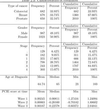
Table 2.3 lists all patient characteristics of interest for both the marginal model and the
missingness model. There are a total of 2010 cancer patients who responded to at least one
of three surveys, including 650 patients with prostate cancer, 682 patients with colorectal
cancer, and 678 patients with breast cancer. The study included three longitudinal surveys.
The cohort includes both male and female whose cancer stage ranges from mild (stage 0) to
severe (stage 4). The age at cancer diagnosis ranges from a minimum of 23 to a maximum of
103. PCIE scores are measured from 8 items; for each item, patients think back to the first
few months of their cancer diagnosis and recall whether they have 1) sought information
about treatments from their treating physician; 2) sought treatment information from other
physicians or health professionals; 3) actively looked for information about their cancer from
their treating physician; 4) actively looked for information about their cancer from other
physicians or health professionals; 5) discussed information from other sources with their
treating physician; 6) received suggestions from their treating physician to get information
from other sources; 7) actively looked for information about quality of life issues from their
treating physician; and 8) looked for quality of life information from other physicians or
health professionals. Each of the 8 items was transformed to a Z-score, and the average of
PCIE score at each times.
The parameters are estimated using the proposed method and compared to a GEE model,
which assumes MCAR missingness, and a WGEE (weighted GEE), which assumes MAR.
Both GEE and WGEE assume an “ignorable” mechanism. The traditional PCIE study
considered the missingness mechanism as either MAR or MCAR, possibly resulting in biased
results. We modify the standard GEE to address missingness in the data. The weighting
is calculated using the missingness mechanism model first, followed by inversion of the
observed probability to form the corresponding weights. The missingness mechanism model
used “cancer type”, “gender”, “age at diagnosis”, “cancer severity”, “PCIE score” and the
previous missingness indicator to predict the current missingness indicator. For “ignorable”
data, WGEE will have unbiased estimators if the underlying data is MCAR. GEE will have
a biased estimators if the underlying data is MAR.
Because missing covariate data was not of primary interest, a multiple imputation method
was used to complete the missing covariates. Rubin (1987) proposed a multiple imputation
method using a Monte Carlo approach in which the missing values are replaced by m >1
simulated versions. We generated m = 20 replicates in our study. Each of the imputed
datasets is analyzed using the proposed method, the GEE model and two weighted GEE
models. The combined parameter estimates and confidence intervals from the m= 20 data
sets follows Rubin’s (Rubin, 1987) multiple imputation rule.
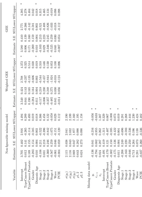
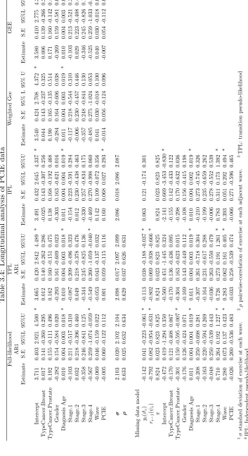
In Table 2.5, we list the parameter estimates after combined 20-fold imputation. The
coeffi-cient forYi in the missingness model indicates if the probability of missingness is related to
the potentially unobserved values of the outcomes. A significant effect indicates that the
lon-gitudinal data is “non-ignorable”. The coefficient forRi−1 indicates if the previous response
had an effect on patients current response. Ri−1= 1 means that the previous response was
collected. Clearly there are statistically significant effects in the missingness model for the
coefficient of both Yi [−0.136(−0.216,−0.055)] and Ri−1 [−0.794(−0.955,−0.633)], which
negative, indicating an inverse relationship with the missingness indicator. Patients who
exercise more tend to be more likely to respond to the survey. They also tend to answer
the questionnaire if they already answered the previous one. Patients who have prostate
cancer [−0.302(−0.595,−0.008)] are more likely to return the questionnaire. Severe cancer
stage (stage 4) [0.713(0.196,1.230)] increases the missingness rate, which indicate that
pa-tients with advanced disease are less likely to respond to the survey. “Wave” has coefficient
[0.287(0.138,0.424)] which suggests that patients tend to be less responsive to the survey
as time increases; this happens typically in repeated measures studies; in that participants
become less compliant as the study advances.
The marginal estimates from our proposed model are somewhat larger than the ones from
either GEE or WGEE model. However, the significance levels are consistent between the
models. Only “age at diagnosis” and “cancer stage” are statistically significant. “Age at
diagnosis” has coefficient 0.010 (0.003,0.018) indicating that older patients engage in more
exercise then younger patients. The coefficient of “cancer stage” [−0.567(−1.075,−0.058)]
indicates a negative correlation with outcome. Patients tend to reduce the amount of
exer-cise when their cancer becomes more severe. PCIE did not show a statistically significant
effect in either model which suggests we did not have enough evidence to show the patients’s
exercise behavior will be affected by differences in the PCIE score.
Although the MCAR and MAR assumption is apparently invalid, both GEE and WGEE
models show similar trends to the proposed model; while most of the parameters estimates
are attenuated, the inferential conclusions are unchanged in this example. The weighted
GEE model provides similar results to the GEE model when the sample size large.
2.4. Simulation Study
2.4.1. Simulation results
In this section we use a simulation study to assess model performance in small samples,
probabilities. We simulated N subjects with three potential measurement times, for N =
300, N = 400 and N = 500. For each setting ofN, we increase the missing rate from low
to high. In the low missingness situation, there is about 10% missing at time 1, 20%−
25% at time 2 , and around 40%−45% missing at time 3. In the higher missingness
setting, there is 30%−35% missing at time 2 and 55%−60% missing at time 3. The
true parameters were selected to fit the proportion of each missingness pattern. Both
the proposed method, the GEE model and weighted GEE model are applied in these six
data settings. 500 simulations have been run to assess the model’s performance; results
are displayed in Table 2.6. The data were generated as trivariate normal, with pairwise
correlation parameters ρ1,2 = 0.4 and ρ2,3 = 0.2. The variance for time 1 is σ1 = 1.2, for
time 2 isσ2 = 2.6 and for time 3 isσ3= 3.0. The estimators are good for both the marginal
parameter and missingness mechanism model in Table 2.6. The bias is very small. Both
GEE and WGEE model consistently underestimate the parameters when the sample size is
small, and the bias is substantial. This becomes much more severe when the missingness
rate increases from low to high. For WGEE model, the weights are calculated through
the missingness mechanism model first, and inverse of the observed probability forms the
weights. “Intercept”, “time” and previous missingness indicator Ri−1 are used to predict
the observed probability. Consistently, WGEE provides better estimators than GEE model
across all data setting, although the bias are still substantial compared with the proposed
model. WGEE model performs better when the missing proportion increases than does the
GEE model.
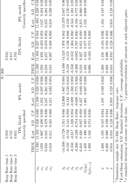
2.4.2. Model Comparison
The proposed model is compared with the original model in Troxel et al. (1998a), which
used the same settings for the complete data and a different logistic model for the
missing-ness indicators denoted as logit(πrit=1) =β0t+β1Yit. In the Troxel et al. (1998a) model,
this missingness model did not include the previous missing indicator as a covariate. We
spec-ified Troxel et al. (1998a) model. The correctly specspec-ified original model from Troxel et al.
(1998a) will become a misspecified model if the coefficient of the previous missing indicator
is not zero. Our proposed model will be over-specified if the parameter of the previous
missing indicator is zero. Table 2.7 shows these comparison results. When the parameter
(ψ) of the previous missing indicator is not zero, the estimates from our transition model are
unbiased and have high coverage probabilities. The Troxel 1998 model has good estimation
in the marginal model and variance-covariance structure, but poor estimation in the
miss-ingness model. This is not surprising, since the missmiss-ingness model is misspecified. When
the parameter (ψ) of the previous missing indicator is zero, both models have very good
estimation. The proposed model uses a small value to estimate the ψ with 95% coverage
rate including zero.
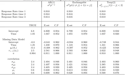
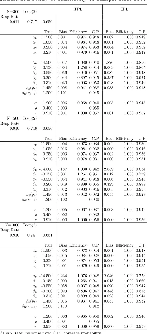
Next, we fit the proposed model with three different covariance structures to see how our
model handles a miss-specified correlation matrix. Our transition model uses ANTE(1)
(ante-dependence) structure denoted as σiσjQk=ij−1ρk for the (i, j)th element. There are a
total of 2t−1 parameters needed. This will become computationally burdensome when t,
the number of repeated times, increases. In practice the AR(1) (autoregressive(1)) structure
is widely used, denoted as σ2ρi−j for the (i, j)th element. There are only two parameters
needed. The Pearson coefficient matrix in Table 2.4 shows the correlation between baseline
and followup is 0.644, and 0.618 for followup2 and followup3. We also have the coefficients
from Table 2.4 for ρ1,2 = 0.643(0.607,0.678) and ρ1,2 = 0.624(0.586,0.662) are statistics
same which make the AR(1) structure reasonable choice. Another two correlation structures
used for comparison are exchangeable (σ2[ρ1(i 6= j) + 1(i = j)]) structure and TOEP(2)
(Banded Toeplitz σ2
The AR(1), exchangeable, and TOEP(2) structure for T = 3 are written respectively as: Σ =
σ2 σ2ρ σ2ρ2
σ2ρ σ2 σ2ρ
σ2ρ2 σ2ρ σ2 AR(1) ; Σ =
σ2 σ2ρ σ2ρ
σ2ρ σ2 σ2ρ
σ2ρ σ2ρ σ2 Exch ; Σ =
σ2 σ1 0
σ1 σ2 σ1
0 σ1 σ2
T OEP(2)
The comparison table is listed in Table 2.8. The proposed model can handle the AR(1)
structure well since it is a special case of ANTE(1) structure. Our model still performs quite
well in estimating the marginal effects and missingness coefficients for both exchangeable
and TOEP(2) structure. The variances are estimated with high coverage probabilities. Both
correlation estimates are less efficient than for the AR(1) model.
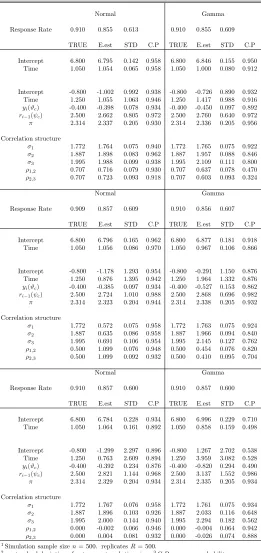
2.4.3. Non-Normal Data
In this section we compared the proposed model to each other with different underlying
assumptions about the data distribution. We simulated two data sets with same true
pa-rameters with different distributions. One data set was simulated from a trivariate normal
distribution. Another was simulated from a trivariate Gamma distribution. A Clayton
copula, which is an asymmetric Archimedean copula, was used to generate the trivariate
Gamma data. This dependence structure of trivariate Gamma followed an exchangeable
correlation. We used Kendall’s formula (Kendall, 1976) to assure the same covariance
struc-ture between trivariate normal and trivariate Gamma data. We generate three correlation
structures with high (ρ = 0.707), low (ρ = 0.5) and zero (ρ = 0) intra-subject correlation
with sample sizes n= 300 andn= 500 to examine the models’ performance in Table 2.9.
Our proposed model performed quite well when the data are normally distributed. The
estimator becomes less efficient when the data are independent (ρ= 0), which makes sense
since the missingness model is miss-specified and thus the model is over-fitted. The marginal
effect and missingness models are still estimated well when the underlying data distribution
is not normal. However, the correlations are poorly estimated, although we still have quite
is strong and worsens when the correlation is weak in the dependent data.
2.5. Discussion
We have presented an extension of the full likelihood-based algorithm to handle
non-monotone and non-ignorable missing data. We assume a first-order Markov structure in
both the complete data and missingness mechanism which is a natural way to capture the
correlation among repeated measurements in a longitudinal data framework. The
estima-tion of marginal effects is generally robust to correct specificaestima-tion of the covariance matrix
and missingness mechanism.
As with any model-based approach to non-ignorable missing data, the current approach is
subject to unavoidable assumptions about the complete data distribution and the missing
data mechanism. It is important to consider all substantive information about the area of
application, prior experience with missing data in similar situations, and expert opinion
about the mechanism of missing data when building such models. In many areas, enough
knowledge and experience exists to justify the necessary assumptions, and the benefit in
terms of bias reduction can be significant.
Our transition model can be easily extended to model more than two states such as dropout
or intermittent missingness. The numerical integration provides an accurate approximation
but at the cost of increased computational complexity. We sometimes encountered a
mul-timodal likelihood surface in our study. A method to handle such surfaces is to choose a
vector of starting values and use GEE estimates to get the starting point as close to the
true values as possible. There are many classes of correlation structure; while we can not
explore all of them, the proposed model can handle the situation of a mis-specified
correla-tion as demonstrated by our simulacorrela-tions. The marginal effects and missingness effects are
consistently estimated with high coverage probability as long as the intra-subject
correla-tion is incorporated. For studies with more than 3 assessment times, it will be difficult to
the model.
There are increasing trends of more and more survey studies to better understand the
rela-tionship of patients, physicians, and the health care system. In most such studies, however,
sample sizes are limited due to restrictions on cancer type, study design and medical
in-formation availability. Small sample sizes with large proportions of missing inin-formation
become more and more concerning for researchers, and limit generalizability. When
in-formation is masked due to reasons relating to the patient-physician relationship, lower
response rates in patients with worse outcomes due to the disease or to accessibility to
medical information and care, special approaches are needed. If data are modeled without
considering this informative missing data, seriously biased inference may result.
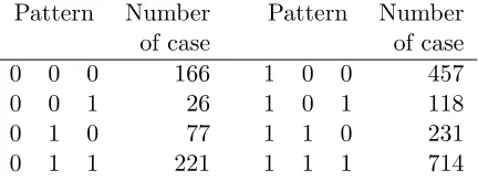
Table 2.1: Missingness patterns in PCIE study Pattern Number Pattern Number
of case of case
0 0 0 166 1 0 0 457
0 0 1 26 1 0 1 118
0 1 0 77 1 1 0 231
0 1 1 221 1 1 1 714
Table 2.2: Response rate for possible outcome Response Rate Exercise PCIE Seeking
Table 2.3: Characteristics of covariates
Type of cancer Frequency Percent Cumulative Cumulative
Frequency Percent
Colorectal 682 33.93% 682 33.93%
Breast 678 33.73% 1360 67.66%
Prostate 650 32.34% 2010 100%
Gender Frequency Percent Cumulative Cumulative
Frequency Percent
Male 987 49.10% 987 49.10%
Female 1023 50.90% 2010 100%
Stage Frequency Percent Cumulative Cumulative
Frequency Percent
. 129 6.42% 129 6.42%
0 182 9.05% 311 15.47%
1 355 17.66% 666 33.13%
2 798 39.70% 1464 72.84%
3 243 12.09% 1707 84.93%
4 303 15.07% 2010 100%
Age at Diagnosis Mean Median Min Max
64.74 65 23 103
PCIE score at time Mean Median Min Max
Wave 1 0.00245 0.00811 -1.27416 1.24094
Wave 2 0.00063 -0.20160 -0.70182 1.88602
Wave 3 0.00167 -0.22578 -0.60372 2.04041
Table 2.4: Pearson correlation matrix of exercise score
Pearson Correlation Coefficients Prob H0: ρ=0
Number of Observations
Wave 1 Wave 2 Wave 3
Wave 1 1 0.6438 0.5848
< .0001 < .0001
1520 945 832
Wave 2 0.6438 1 0.6184
< .0001 < .0001
945 1243 935
Wave 3 0.5848 0.6184 1
< .0001 < .0001
T able 2.5: Longitudinal analysis of PCIE data Non-Ignorable missing mo del W eigh ted GEE GEE V ariable Estimate S.E 95%Lo w er 95%upp er Estimate S.E 95% Lo w er 95%upp er Estimate S.E 95%Lo w er 95%upp er In tercept 3.705 0.402 2.916 4.494 * 3.540 0.424 2.708 4.372 * 3.580 0.410 2.775 4.385 * T yp eCancer.Breast 0.012 0.141 -0.265 0.289 0.044 0.143 -0.237 0.325 0.006 0.139 -0.266 0.278 T yp eCancer.Prostate 0.189 0.155 -0.114 0.493 0.190 0.165 -0.135 0.514 0.171 0.160 -0.142 0.484 Gender -0.283 0.154 -0.585 0.019 -0.284 0.164 -0.606 0.038 -0.269 0.159 -0.581 0.042 Dianosis Age 0.010 0.004 0.003 0.018 * 0.011 0.004 0.003 0.019 * 0.010 0.004 0.003 0.018 * Stage.1 -0.108 0.211 -0.522 0.306 -0.117 0.218 -0.544 0.310 -0.103 0.213 -0.521 0.315 Stage.2 0.031 0.218 -0.396 0.458 -0.006 0.230 -0.457 0.446 0. 02 9 0.223 -0.408 0. 465 Stage.3 -0.360 0.246 -0.842 0.122 -0.357 0.248 -0.844 0.130 -0.346 0.245 -0.826 0.134 Stage.4 -0.567 0.259 -1.075 -0.058 * -0.485 0.275 -1.024 0.053 * -0.525 0.259 -1.033 -0.018 * W a v e -0.061 0.046 -0.151 0.029 0.041 0.030 -0.018 0.100 0.040 0.030 -0.018 0.098 PCIE -0.004 0.059 -0.120 0.112 -0. 014 0.056 -0.124 0.096 -0.007 0.054 -0.112 0.098 σ ( y1 ) 2.115 0.038 2.041 2.190 σ ( y2 ) 2.116 0.043 2.032 2.199 σ ( y3 ) 2.069 0.047 1.977 2.160 ρ 1 , 2 0.643 0.282 0.090 1.195 ρ 2 , 3 0.624 0.273 0.090 1.158 Missing data mo del yi -0.136 0.041 -0.216 -0.056 *
ri−
Table 2.6: Simulation study 500 replicates N=300
Response Rate Time 1 Time 2 Time 3 Time 1 Time 2 Time 3 0.909 0.840 0.605 0.911 0.681 0.434
Full Liklihood GEE WGEE Full Liklihood GEE WGEE TRUE E.est C.P Bias E.est Bias E.est Bias TRUE E.est C.P Bias E.est Bias E.est Bias
Intercept 6.800 6.793 0.950 0.007 6.308 0.492 6.393 0.407 5.600 5.604 0.948 0.004 4.996 0.604 5.134 0.466 Time 1.050 1.062 0.956 0.012 1.518 0.468 1.445 0.395 0.300 0.301 0.942 0.001 0.914 0.614 0.782 0.482
Missingness model
Intercept -0.800 -0.990 0.958 0.190 -0.800 -0.894 0.952 0.094 Time 1.250 1.103 0.952 0.147 1.250 1.213 0.956 0.037
yi(ϑc) -0.400 -0.404 0.936 0.004 -0.400 -0.412 0.950 0.012
ri−1(ψc) 2.500 2.676 0.976 0.176 2.500 2.628 0.962 0.128
π 2.314 2.326 0.934 0.012 2.314 2.363 0.946 0.049
Correlation structure
σ1 0.182 0.181 0.950 0.002 0.182 0.179 0.952 0.004
σ2 0.956 0.953 0.944 0.003 0.956 0.953 0.948 0.002
σ3 1.099 1.095 0.952 0.004 1.099 1.099 0.946 0.001
ρ1,2 0.847 0.849 0.922 0.002 0.847 0.853 0.952 0.006
ρ2,3 0.405 0.414 0.940 0.009 0.405 0.408 0.938 0.002
N=400
Response Rate Time 1 Time 2 Time 3 Time 1 Time 2 Time 3 0.911 0.826 0.593 0.910 0.668 0.425
Full Liklihood GEE WGEE Full Liklihood GEE WGEE TRUE E.est C.P Bias E.est Bias E.est Bias TRUE E.est C.P Bias E.est Bias E.est Bias
Intercept 6.400 6.402 0.942 0.002 5.913 0.487 6.001 0.399 5.400 5.402 0.930 0.002 4.788 0.612 4.919 0.481 Time 1.100 1.100 0.932 0.000 1.571 0.471 1.494 0.394 0.300 0.300 0.936 0.000 0.917 0.617 0.789 0.489
Missingness model
Intercept -0.800 -0.867 0.954 0.067 -0.800 -0.905 0.956 0.105 Time 1.250 1.224 0.960 0.026 1.250 1.205 0.942 0.045
yi(ϑc) -0.400 -0.410 0.920 0.010 -0.400 -0.407 0.940 0.007
ri−1(ψc) 2.500 2.600 0.950 0.100 2.500 2.612 0.948 0.112
π 2.314 2.340 0.960 0.027 2.314 2.339 0.972 0.025
Correlation structure
σ1 0.182 0.179 0.950 0.003 0.182 0.180 0.950 0.002
σ2 0.956 0.956 0.938 0.000 0.956 0.949 0.950 0.006
σ3 1.099 1.098 0.942 0.000 1.099 1.094 0.946 0.004
ρ1,2 0.847 0.854 0.942 0.007 0.847 0.846 0.954 0.001
ρ2,3 0.405 0.409 0.932 0.003 0.405 0.409 0.958 0.003
N=500
Response Rate Time 1 Time 2 Time 3 Time 1 Time 2 Time 3 0.911 0.805 0.587 0.910 0.666 0.427
Full Liklihood GEE WGEE Full Liklihood GEE WGEE TRUE E.est C.P Bias E.est Bias E.est Bias TRUE E.est C.P Bias E.est Bias E.est Bias
Intercept 5.600 5.591 0.940 0.009 5.111 0.489 5.202 0.398 5.400 5.404 0.952 0.004 4.787 0.613 4.918 0.482 Time 1.300 1.309 0.934 0.009 1.778 0.478 1.698 0.398 0.300 0.295 0.954 0.005 0.917 0.617 0.788 0.488
Missingness model
Intercept -0.800 -0.907 0.932 0.107 -0.800 -0.872 0.920 0.072 Time 1.250 1.164 0.938 0.086 1.250 1.226 0.940 0.024
yi(ϑc) -0.400 -0.403 0.946 0.003 -0.400 -0.410 0.962 0.010
ri−1(ψc) 2.500 2.606 0.952 0.106 2.500 2.600 0.964 0.100
π 2.314 2.334 0.938 0.020 2.314 2.347 0.936 0.033
Correlation structure
σ1 0.182 0.178 0.960 0.004 0.182 0.177 0.944 0.006
σ2 0.956 0.956 0.944 0.000 0.956 0.957 0.946 0.001
σ3 1.099 1.096 0.938 0.003 1.099 1.094 0.944 0.004
ρ1,2 0.847 0.850 0.958 0.002 0.847 0.845 0.948 0.003
ρ2,3 0.405 0.405 0.950 0.001 0.405 0.417 0.948 0.011 1σ
Table 2.7: Model comparison simulations, 1000 replicates N=300
Res.Rate time 1 0.9095 0.9102
Res.Rate time 2 0.8395 0.8806
Res.Rate time 3 0.6042 0.6368
Transition Model Troxel 1998 model Transition Model Troxel 1998 model
correctly specified correctly specified
Parameter TRUE E.est C.P E.est C.P TRUE E.est C.P E.est C.P Intercept 6.8 6.798 0.944 6.711 0.926 1.8 1.788 0.931 1.780 0.932
time 1.05 1.048 0.935 1.133 0.911 1.05 1.062 0.931 1.070 0.933 Missingness Model
Intercept -0.8 -0.948 0.954 0.721 0.575 -0.8 -1.115 0.941 -0.919 0.958 Time 1.25 1.145 0.943 2.397 0.852 1.25 1.022 0.944 1.190 0.949
yi(ϑc) -0.4 -0.410 0.932 -0.289 0.785 -0.4 -0.407 0.950 -0.396 0.942 ri−1(ψc) 2.5 2.674 0.963 - - 0 0.229 0.959 -
-π 0.91 0.910 1.000 0.910 1.000 0.91 0.914 1.000 0.916 1.000 Correlation
σ1 1.2 1.195 0.967 1.196 0.968 1.2 1.195 0.940 1.194 0.940
σ2 2.6 2.593 0.948 2.549 0.919 2.6 2.594 0.936 2.586 0.936
σ3 3 3.001 0.940 2.949 0.932 3 2.997 0.928 2.978 0.929
ρ1 0.4 0.398 0.953 0.400 0.950 0.4 0.400 0.948 0.402 0.948
ρ2 0.2 0.202 0.948 0.207 0.942 0.2 0.196 0.940 0.196 0.940 1Simulation sample sizen= 300. replicates 1000. Res.Rate: Response Rate 2σ
istandard deviation of outcome at
each timei. 3C.P coverage probability. 4E.estMean estimation.
Table 2.8: Simulation comparison study, 500 replicates
AR(1) Exchangable Toep(2) σ2ρi−j σ2[ρ1(i6=j) + 1(i=j)] σ2
|i−j|+11(|i−j|<2)
Response Rate time 1 0.910 0.910 0.910 Response Rate time 2 0.844 0.844 0.844 Response Rate time 3 0.614 0.616 0.610
TRUE E.est C.P E.est C.P E.est C.P
Intercept 6.8 6.809 0.954 6.799 0.954 6.809 0.932 Time 1.05 1.047 0.952 1.055 0.970 1.037 0.920
Missing Data Model
Intercept -0.8 -0.841 0.962 -0.934 0.960 -0.749 0.944 Time 1.25 1.238 0.970 1.123 0.954 1.331 0.966 yi(ϑc) -0.4 -0.408 0.962 -0.397 0.952 -0.423 0.948
ri−1(ψc) 2.5 2.581 0.966 2.593 0.968 2.622 0.948
π 0.904 0.911 1.000 0.911 1.000 0.910 1.000
correlation
σy1 2.4 2.404 0.946 2.401 0.946 2.403 0.960
σy2 2.4 2.407 0.956 2.421 0.944 2.385 0.956
σy3 2.4 2.405 0.930 2.405 0.956 2.403 0.956
ρ1 0.6 0.600 0.954 0.613 0.932 0.583 0.920
ρ2 0.6 0.600 0.962 0.620 0.894 0.568 0.876 1Simulation sample sizen= 500. replicatesR= 500. 2σ
istandard deviation of outcome at each timei.
Table 2.9: Non-normal data, 500 replicates
Normal Gamma
Response Rate 0.910 0.855 0.613 0.910 0.855 0.609
TRUE E.est STD C.P TRUE E.est STD C.P
Intercept 6.800 6.795 0.142 0.958 6.800 6.846 0.155 0.950 Time 1.050 1.054 0.065 0.958 1.050 1.000 0.080 0.912
Intercept -0.800 -1.002 0.992 0.938 -0.800 -0.726 0.890 0.932 Time 1.250 1.055 1.063 0.946 1.250 1.417 0.988 0.916
yi(ϑc) -0.400 -0.398 0.078 0.934 -0.400 -0.450 0.097 0.892
ri−1(ψc) 2.500 2.662 0.805 0.972 2.500 2.760 0.640 0.972
π 2.314 2.337 0.205 0.930 2.314 2.336 0.205 0.956
Correlation structure
σ1 1.772 1.764 0.075 0.940 1.772 1.765 0.075 0.922
σ2 1.887 1.898 0.083 0.962 1.887 1.957 0.088 0.846
σ3 1.995 1.988 0.099 0.938 1.995 2.109 0.111 0.800
ρ1,2 0.707 0.716 0.079 0.930 0.707 0.637 0.078 0.470
ρ2,3 0.707 0.723 0.093 0.918 0.707 0.603 0.093 0.324
Normal Gamma
Response Rate 0.909 0.857 0.609 0.910 0.856 0.607
TRUE E.est STD C.P TRUE E.est STD C.P
Intercept 6.800 6.796 0.165 0.962 6.800 6.877 0.181 0.918 Time 1.050 1.056 0.086 0.970 1.050 0.967 0.106 0.866
Intercept -0.800 -1.178 1.293 0.954 -0.800 -0.291 1.150 0.876 Time 1.250 0.876 1.395 0.942 1.250 1.964 1.332 0.876
yi(ϑc) -0.400 -0.385 0.097 0.934 -0.400 -0.527 0.153 0.862
ri−1(ψc) 2.500 2.724 1.010 0.988 2.500 2.868 0.696 0.982
π 2.314 2.323 0.204 0.944 2.314 2.338 0.205 0.932
Correlation structure
σ1 1.772 0.572 0.075 0.958 1.772 1.763 0.075 0.924
σ2 1.887 0.635 0.086 0.958 1.887 1.966 0.094 0.840
σ3 1.995 0.691 0.106 0.954 1.995 2.145 0.127 0.762
ρ1,2 0.500 1.099 0.076 0.948 0.500 0.454 0.076 0.820
ρ2,3 0.500 1.099 0.092 0.932 0.500 0.410 0.095 0.704
Normal Gamma
Response Rate 0.910 0.857 0.600 0.910 0.857 0.600
TRUE E.est STD C.P TRUE E.est STD C.P
Intercept 6.800 6.784 0.228 0.934 6.800 6.996 0.229 0.710 Time 1.050 1.064 0.161 0.892 1.050 0.858 0.159 0.498
Intercept -0.800 -1.299 2.297 0.896 -0.800 1.267 2.702 0.538 Time 1.250 0.763 2.609 0.894 1.250 3.959 3.082 0.528
yi(ϑc) -0.400 -0.392 0.234 0.876 -0.400 -0.820 0.294 0.490
ri−1(ψc) 2.500 2.821 1.144 0.968 2.500 3.137 1.552 0.986
π 2.314 2.329 0.204 0.934 2.314 2.335 0.205 0.934
Correlation structure
σ1 1.772 1.767 0.076 0.958 1.772 1.761 0.075 0.934
σ2 1.887 1.896 0.103 0.926 1.887 2.033 0.116 0.648
σ3 1.995 2.000 0.144 0.940 1.995 2.294 0.182 0.562
ρ1,2 0.000 -0.002 0.066 0.946 0.000 -0.004 0.064 0.942
ρ2,3 0.000 0.004 0.081 0.932 0.000 -0.026 0.074 0.888 1Simulation sample sizen= 500. replicatesR= 500.
2σ