235 | P a g e
EFFICIENT & ANALYSIS OF PCA BASED IMAGE
CHANGE DETECTION ALGORITHMS
Saravanan M
1, Santhosh Sivan M.A
21
Associate Prof.,
2UG Student, Computer Science,
K.R.College of Arts & Science, Kovilpatti, Tamilnadu (India)
ABSTRACT
Recent change detection techniques rely either on supervised or unsupervised techniques. The first requires
ground truth samples to train a classifier. The second approach relies on automatic techniques including
thresholding or clustering on a combination of the bi-temporal images. Principal component analyses (PCA)
has been widely used in reduction of the dimensionality of datasets, classification, feature extraction, etc. It has
been combined with many other algorithms such as EM (expectation-maximization), ANN (artificial neural
network), probabilistic models, statistic analyses, etc., and has its own development such as MPCA (moving
PCA), MS-PCA (multi-scale PCA), etc. PCA–and its derivatives- has a wide range of applications, from face
detection to change analysis. Change detection from PCA shows, however, a main difficulty, that is, result
interpretation. In this project, a new PCA method is developed, namely MB-PCA (Multi-Block PCA), in order to
overcome this problem. Experimental results demonstrate the interest of the approach as a new way to use PCA.
Keywords: Land cover changes, Principal Component Analysis, PCA, Multi-block PCA, Change
Detection Algorithms
I. INTRODUCTION
Change Detection (CD) is the process of identifying differences in the state of an object or phenomenon by observing it at different times [5]. It is an important application of remote sensing in environmental monitoring and defence areas. Researchers have been trying to develop efficient and accurate procedures to detect and label the changes in multi-spectral or single band image sets taken at two or more different times. Here we used PCA based CD algorithms [4][13][15] to analyse the performance of identifying the land cover changes of Madurai city and man made imagery. Land cover implies the physical or natural state of the Earth‟s surface, i.e, what is actually present on the ground and may also contain an ecological description [5].
236 | P a g e
The first part of the paper briefly introduces the background of change detection. This is followed by a description about the study area and data. The third section gives methodology adapted; followed by results and discussions and finally by the conclusion.
1.1 Study area and data description
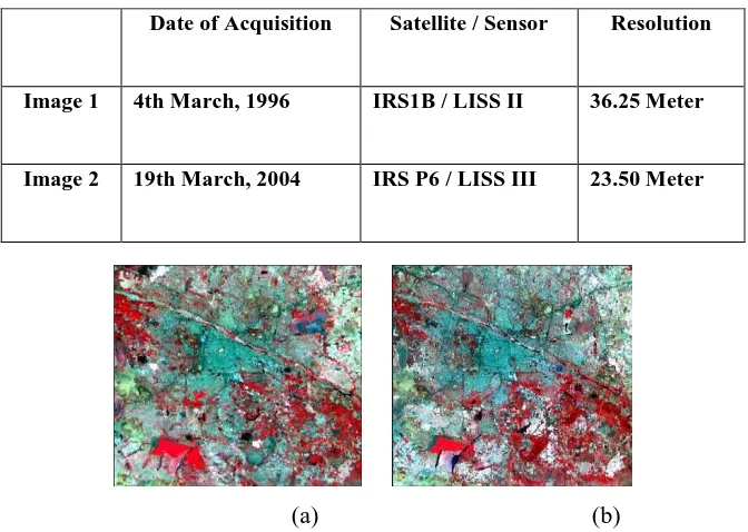
By the help of some tools of Adobe Photoshop we did some changes in the still images (captured by a camera). The size of each image should be restricted because the size should be easily divisible to produce the number of sub-blocks. Six still images and two remotely sensed images taken in different date/time were chosen as input images for our experiment. The selected area for the remotely sensed input images for this research is the Madurai city, Tamilnadu, India. Madurai is a historical city and it is the gateway of south Tamilnadu. It is one of the mini metros in India. The city is well known for its architectural marvels and its rich cultural heritage. The city is known as the Athens of East. Madurai is situated between the longitude 78° 04‟ 47” E to 78° 11‟ 23” E and the latitude 9° 50‟ 59” N to 9° 57‟ 36” N. The topography of Madurai is approximately 101 meters above the sea level. The city lies in the interior of Tamilnadu. The present area of the city is 51.9 square kilometers. Now due to economic advancement of the people of the city the rural hamlets in the district are given an urban image by people. With the view to present an analytical perspective for the socio economical issues pertaining to Madurai, it is needed to analyse the spatial pattern such as urban sprawl, to predict the future growth. The kinds of satellite data with different resolution and acquisition dates (LISS II and LISS III) were used in this research is given in table 1. The pre-processed multispectral temporal input image data is shown in figure1.
TABLE 1 - Input image Resolution
(a)
(b)
Figure 1 Input images (a)LISS II image – 1996; (b) LISS III image – 2004
II. METHODOLOGY
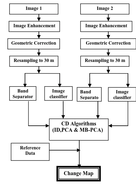
The proposed approach to evaluate the performance of CD algorithms consisted of three steps: 1) Image Pre-processing, 2) Band Separation and 3) Apply CD algorithm. Prior to application of change detection
Date of Acquisition Satellite / Sensor Resolution
Image 1 4th March, 1996 IRS1B / LISS II 36.25 Meter
237 | P a g e
algorithms, the two satellite images should be normalized by using pre-processing techniques like image enhancement, geometric correction and re-sampling. After pre-processing process, these images were subjected to band separation. Red band of both satellite images were used in the image differencing where as infra-red and red bands were used for urban change detection. In PCA, Hotelling transformation[19][20] was applied to both the satellite images and the transformed images were subjected to image differencing algorithm for further analysis. Each principal component of the resultant image was analysed to identify land cover changes of Madurai city. Recent research has also directed its effort in the development of varieties of alternate PCA techniques, namely, Multiscale PCA, and Multiblock PCA (MB-PCA)[17].
Multiblock PCA applies to large processes that are composed of a multitude of units and thus many variables per unit. The method decomposes the whole unit into blocks of variables, which are highly coupled within block, and least coupled different blocks. This method makes it easier to diagnose and detect the changed regions. An earlier example of the method is found in MaxGregor et al[9]. A more recent application of Multiblock PCA in semiconductor process is in two-level multiblock statistical monitoring for plant-wide processes, as well as Perk and Cinar. Because of facing many difficulties in explaining the results of the traditional PCA method when doing change detection, especially when having to give out the differences between PC1 and PC2, we put forward a new idea in processing PCA to try to solve such a problem both in the theory and in its application field. In the past literatures, there exists such a word „multi-block‟ PCA[11], but its meaning is totally different from ours. It was developed under the name Consensus-PCA in process monitoring. The block diagram of the proposed system is shown in figure 2.
Figure 2 Proposed System
Image 1 Image 2
Image Enhancement Image Enhancement
Geometric Correction Geometric Correction
Resampling to 30 m Resampling to 30 m
Band Separator
( ID, IR, CVA)
Image classifier
Band Separato r ( ID, IR, CVA)
Image classifier
CD Algorithms (ID,PCA & MB-PCA)
Change Map
238 | P a g e
2.1 Image Differencing
Image differencing requires that each pixel value of an image be subtracted from its corresponding pixel value of another image[9] . The resultant image represents the change between the two times. Image differencing may be applied to a single band (univariate image differencing) or to multiple bands and it is an effective algorithm in evaluating the urban changes [14]. The accuracy of the image differencing algorithms could be improved by including texture information [3]. References [1] and [2] show that image differencing have good results compared to PCA in urban environment. Rajesh Acharya stated image differencing is a rather straight forward and simple approach. Through this study only we used red band, it successfully differentiates the area as change and no-change. The limitation of this algorithm is the immediate identification of the change area but not the type of the change.
2.2 Principal Component Analysis (PCA)
Principal component comparison is one of the most popular multivariate analysis algorithms for change detection studies [4]. PCA is performed on the image data of each date. The derived principal components are again analysed by applying other CD methods such as image differencing and regression methods. The PCA can be performed on original or standardized data. The former uses the covariance matrices, while the later uses the correlation matrices. If the original data is used, PC1 usually has equal loading on all spectral bands and PC2 represents the difference between visible and infrared bands. If the standardized data is used, PC2 usually has equal loading on all spectral bands and PC1 represents the difference between visible and infrared bands. There are some steps for implementing PCA [16]. They are:
1. Take an original data set and calculate mean of the data set: Taking X1, X2, … XN as column vectors,
each of which has M rows. Place the column vectors into a single matrix X of dimensions M × N.
2. Subtract off the mean for each dimension: Find the empirical mean along each dimension m = 1, ..., M of each column. Place the calculated mean values into an empirical mean vector u of dimensions M × 1.
Mean subtraction is an integral part of the solution towards finding a principal component basis that minimizes the mean square error of approximating the data. There are two steps:
Subtract the empirical mean vector u from each column of the data matrix X.
Store mean-subtracted data in the M*N matrix B. B = X - uh
[Where h is a 1 x N row vector of all 1's : h[n] = 1 for n = 1…N]
3. Calculate the covariance matrix: Find the M×M covariance matrix C from the outer product of matrix B with itself:
C = E[B×B] = E[B.B*] = (1/N) ΣB.B*
where E is the expected value operator, × is the outer product operator, and * is the conjugate transpose operator. Note that if B consists entirely of real numbers, which is the case in many applications, the "conjugate transpose" is the same as the regular transpose.
239 | P a g e
V-1CV = D
where D is the diagonal matrix of eigen values of C. This step will typically involve the use of a computer-based algorithm for computing eigenvectors and eigen values.
5. Extract diagonal of matrix as vector: Matrix D will take the form of an M × M diagonal matrix, where D[p,q] = λm for p = q = m is the mth eigenvalue of the covariance matrix C, and D[p,q] = 0 for p ≠ q matrix V, also of dimension M × M, contains M column vectors, each of length M, which represent the M eigenvectors of the covariance matrix C.
6. Sorting in variance in decreasing order: Sort the column of the eigen vector matrix V and eigen value matrix D in order of decreasing eigen value
7. Choosing components and forming a feature vector: Here is where the notion of data compression and reduced dimensionality comes into it. If we look at the eigenvectors and eigen values from the previous section, we will observe that the eigen values are quite different values. In fact, it turns out that the eigenvector with the highest eigen value is the principle component of the data set. What needs to be done now is you need to form a feature vector. Taking the eigenvectors that we want to keep from the list of eigenvectors, and forming a matrix with these eigenvectors in the columns construct this:
FeatureVector = (eig1 eig2 eig3……….eign)
8. Deriving the new data set: This is the final step in PCA and it is also the easiest. Once we have chosen the components (eigenvectors) that we wish to keep in our data and formed a feature vector, we simply take the transpose of the vector and multiply it on the left of the original data set, transposed. FinalData = RowFeatureVector* RowDataAdjust where RowFeatureVector is the matrix with the eigenvectors in the columns transposed so that the eigenvectors are now in the rows, with the most significant eigenvectors at the top, and RowDataAdjust is the mean-adjusted data transposed, i.e. the data items are in each column, with each row holding a separate dimension.
2.3 Multi-Block PCA (MB-PCA)
Because of facing many difficulties in explaining the results of the traditional PCA method when doing change detection, especially when having to give out the differences between PC1 and PC2, we put forward a new idea in processing PCA to try to solve such a problem both in the theory and in its application field. In the past literatures, there exists such a word „multi-block‟ PCA[16], but its meaning is totally different from ours. It was developed under the name Consensus-PCA in process monitoring. But what we mean here is to do PCA process as following four steps [17]:
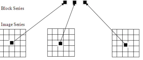
Partition: Beginning from a series of images (X1, …, Xn)t, we divide each Xi into a group of sub-images or blocks (BXi1, …, BXim), i Є [1, n]. Then all the blocks (BXij), iЄ [1, n], j Є [1, m], constitute the same matrix as
A=(X1, …, Xn)t, which means A = (BXij).
Group:In matrix A, while fixed its row i, it is exactly the image Xi; while fixed its column j, (BX1j, …, BXnj)
can be regarded as a sub-image / block series extracted from the initial images (X1, …, Xn)t, which can be seen
240 | P a g e
Block PCA: In this step, we apply PCA analysis on those m block series separately. For example, in series j, (BX1j, …, BXnj), j Є [1, m], after PCA process we can get n principle components such as (BPC1, BPC2, …,
BPCn), whose corresponding eigen values are ranked in descending orders.
Combination: After all the m series are processed, we obtain m BPC1s, which can be constructed into a new
image — PC1. Similarly, all the m BPC2s can be constructed into image PC2, and so as to the other PCs. Thus
we can obtain n new constructed images (PC1, PC2, …, PCn). It is obvious that those images have the same size
as the initial images (X1, …, Xn). Inside all of the new images, PC1 is the most important one.
Figure 3 Block image series (there are n images in total and for each image there are m blocks)
III RESULTS AND DISCUSSION
After pre-processing, multivariate image differencing algorithm was applied to produce change map between temporal images, as shown in figure 4(a). PCA was performed on pre-processed multivariate image data of each date individually. Then the derived principal components (PC1) were again analysed by applying image differencing algorithm. The result of PCA is shown in figure 4(b). MB-PCA was performed on pre-processed multivariate image data of each date individually. Then the newly constructed, PC1, principal component of multivariate input images were again analysed by applying image differencing algorithm. The result of MB-PCA is shown in figure 4(c). The no-change (NC) areas in a change map were represented in black colour, where as the change areas were again divided into increased change(IC), represented in red colour, and decreased change(DC), represented in green colour. The used threshold value to distinguish change and no-change pixels between two dates and the number of pixels of each category were tabulated.
3.1. Performance Analysis
Here, performance evaluation is mainly used to compare different techniques under image processing. The performance analysis is carried out by considering the elapsed time to do the algorithm for man-made input mages and the verification of ground truth with the result for satellite image.
Before analysing the results upwards, we should review the general interpretation for traditional PCA. If the eigenvalue of PC1 is much bigger than the others, PC1 should be the background/common part of all the images
(X1, … , Xn), and could show the „stable‟ and „unchangeable‟ part of the whole image series. So it can be
regarded as the „background‟ of the whole image series. Now let‟s consider the combined image PC1 obtained
from the four steps given in MB-PCA. For each sub-block (BPC1) of it, if its eigenvalue is much bigger than
those in (BPC2, …, BPCn), it means it is the background / common part of all its block image series (BX1j, …,
BXnj). On the other hand, if its eigenvalue is near to some others of (BPC2, …, BPCn), it means it is a changed
241 | P a g e
If all the regions are similar to each other, the rank of the block series matrix will be near to 1. Then in thesame block series the eigenvalue of B-PC1 will be much bigger than all the other eigenvalues of BPCi.
Conversely, if the calculated result of eigenvalue of BPC1 is much bigger than all the others, we can
conclude there is no obvious change in this region. And across the block series, this small region keeps nearly the same.
If there are some changes in this small region, which means that there are more than one type in the block series but not only the pure background, the eigenvalue of BPC1 will not be so prominent compared with
others. Conversely, if the eigen values are near to each other, it means that there exists a change in this region.
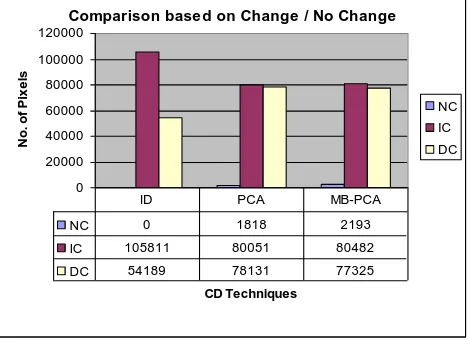
From the two rules we can conclude that the distribution of eigen values of block series shows if there exists a change across the image series. The number of change and no-change pixels produced by using image differencing, PCA and MB-PCA methods were tabulated and the column chart was given in figure 4 for the purpose of efficiency analysis of the above three methods.
3.2 Accuracy Assessment
In the final step of implementation, the resulting change map of each part, and ground truth were applied to form an error matrix for accuracy assessment. The selection of the better algorithm for land cover change detection should be based on the accuracy of classifying the pixels as change or no-change. Most of the researchers recommend the use of the kappa coefficient of agreement as the standard measure for accuracy. The error matrix for image differencing, PCA and MB-PCA are given in table 2. From the above mentioned CD algorithms, the MB-PCA gave the better result with over all kappa, K = 0.71 than the PCA and image differencing.
Comparison based on Change / No Change
0 20000 40000 60000 80000 100000 120000
CD Techniques
N
o
.
o
f
Pi
x
e
ls
NC IC DC
NC 0 1818 2193
IC 105811 80051 80482
DC 54189 78131 77325
ID PCA MB-PCA
Figure 4 Comparison of ID, PCA, MB-PCA methods
IV CONCLUSION
242 | P a g e
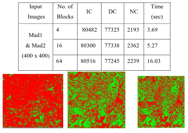
intensity changes in those same regions. A point we should mention is the computational cost. Compared with traditional PCA process, multi-block PCA has increased computation time obviously. If we increased the number of blocks or sub-images to 16 or 64, the elapsed time to find the change and no-change pixels would be 5.27 sec and 16.03 sec respectively (See Table 3).
This method is still under development. And there is some further work to do, such as the influence of the block sizes, block shapes, etc. To model an intensity transformation to eliminate the influence of light-change is also an interesting work. At the other hand, we only used one channel dataset until now, and in fact there are multi-sensorial and multi-temporal satellite images available[17][18][19][20]. How to apply Multi-block PCA method on those dataset to detect change is a good direction.
TABLE 3 RESULT OF MB-PCA TECHNIQUE
Input Images
No. of
Blocks IC DC NC
Time (sec) Mad1
& Mad2 (400 x 400)
4 80482 77325 2193 3.69 16 80300 77338 2362 5.27 64 80516 77245 2239 16.03
Figure 4 Change Map images (a) Image Differencing (b) PCA (c) MB-PCA
Table 2 Confusion Matrices obtained for ID, PCA, MB-PCA
Image Differencing PCA MB-PCA
NC DC IC K NC DC IC K NC DC IC K
NC 0 9 14 -.01 20 4 3 0.10 21 6 2 0.10
DC 1 18 11 0.07 3 30 5 0.15 3 25 4 0.12
IC 12 16 69 0.09 11 2 72 0.25 7 4 78 0.28
Over all Kappa 0.30 0.69 0.71
REFERENCES
[1] Abdullah Almutairi, Monitoring land-cover changes: a comparison of change detection techniques, Univ. of West Virginia, 2000.
243 | P a g e
[3] Jenson.J.R., Introductory Digital Image Processing: a remote sensing perspective, 3rd ed., Ch.12 Digital Change Detection, pp.467-494, 2005.
[4] Lindey I Smith, A tutorial on Principal Component Analysis, 2002.
[5] Singh.A, Digital Change Detection Techniques using Remotely sensed data, Int.J.Remote Sensing, vol.10 no.6, pp.989-1003, 1989
[6] Volpi et al (2009), Supervised Change Detection in VHR images: A comparative analysis, IEEE MLSP. [7] M. Volpi, D. Tuia, M.Kanevski, F.Bovolo, and L.Bruzzone, “ Supervised Change detection in VHR
images using contextual information and support vector machines”, Int. J. Appl. Earth. Obs., vol. DOI: 10.1016/j.jag.2011.10.013, 2011
[8] Liu S.C., Fu C.W., Chang S.Y., “Statistical Change Detection with Moments Under Time-Varying Illumination”, IP(7), No. 9, 9 (1998), pp. 1258-1268.
[9] West erhuis J.A., Kourti T. and MaxGregor J.F., “Analysis of multiblock and hierarchical PCA and PLS models”, Journal of Chemometrics, 12 (1998), 463-482.
[10] Bruzzone, L., Serpico, S.B., “Detection of Changes in Remotely-Sensed Images by the Selective Use of Multispectral Information”, JRS (18), No. 18, 12 (1997), pp. 3883-3888.
[11] Chen L.C., Rau J.Y., “Detection of shoreline changes for tideland areas using multi-temporal satellite images”, JRS (19), No. 17, 9 (1998), pp. 3383.
[12] Igbokwe J.I., “Geometrical processing of multi-sensoral multi-temporal satellite images for change detection studies”, JRS (20), No. 6, 4 (1999), pp. 1141.
[13] Jonathon Shiens, “A Tutorial on Principal Component Analysis” Centre for Neural Science, New York University, 22nd April 2009, Version 3.01.
[14] Dale P.E.R. etc, “Using Image Subtraction and Classification to Evaluate Change in Subtropical Intertidal Wetlands”, JRS (17), No. 4, 3(1996), pp. 703-719.
[15] Michael Collins, Sanjoy Dasgupta, Robert E. Schapire, “A Generalization of Principal Component Analysis to the Exponential Family”, NIPS2001, http://www-2.cs.cmu.edu/Groups/NIPS/NIPS2001
/papers .
[16] Abhishek Banerjee, “Impact of PCA in the Application of Image Processing”, IJARCSSE, vol.2 issue 1, Jan 2013 ISSN2277 128X
[17] Qui .B, Prinet .V, Monga .O, “Multi-Block PCA Method for Image Change Detection”, Proceedings of the 12th International Conference on Image Analysisand Processing (ICIAP‟03), 0-7695-1948-2/03 ©IEEE Computer Society
[18] Saravanan .M “Peformance Analysis of Change Detection Algorithms using Remote Sensing Images”, Proceedings of the first International Conference on Advanced Computing (ICAC‟14), 2014.
[19] Saravanan .M, Sundareswaran .P, “A Peformance Analysis of supervised Change Detection Algorithms ,Proceedings of the fifth National Conference on Recent Trends in Information Technology (NCRTIT‟11), March vol.05,pp.117-122, 2011