New Hampshire Agricultural Experiment Station
Research Institutes, Centers and Programs
1-12-2016
GBS-SNP-CROP: a reference-optional pipeline for
SNP discovery and plant germplasm
characterization using variable length, paired-end
genotyping-by-sequencing data
Arthur Tavares De Oliveira Melo
University of New Hampshire, Durham, [email protected]
Radhika Bartaula
University of New Hampshire, Durham
Iago L. Hale
University of New Hampshire, Durham, [email protected]
Follow this and additional works at:
https://scholars.unh.edu/nhaes
This Article is brought to you for free and open access by the Research Institutes, Centers and Programs at University of New Hampshire Scholars' Repository. It has been accepted for inclusion in New Hampshire Agricultural Experiment Station by an authorized administrator of University of New Hampshire Scholars' Repository. For more information, please [email protected].
Recommended Citation
Arthur T. O. Melo, Radhika Bartaula and Iago Hale. GBS-SNP-CROP: a reference-optional pipeline for SNP discovery and plant germplasm characterization using variable length, paired-end genotyping-by-sequencing data. BMC Bioinformatics (2016) 17:29.
M E T H O D O L O G Y A R T I C L E
Open Access
GBS-SNP-CROP: a reference-optional
pipeline for SNP discovery and plant
germplasm characterization using variable
length, paired-end
genotyping-by-sequencing data
Arthur T. O. Melo
1, Radhika Bartaula
2and Iago Hale
1*Abstract
Background:With its simple library preparation and robust approach to genome reduction, genotyping-by-sequencing (GBS) is a flexible and cost-effective strategy for SNP discovery and genotyping, provided an appropriate reference genome is available. For resource-limited curation, research, and breeding programs of underutilized plant genetic resources, however, even low-depth references may not be within reach, despite declining sequencing costs. Such programs would find value in an open-source bioinformatics pipeline that can maximize GBS data usage and perform high-density SNP genotyping in the absence of a reference.
Results:The GBS SNP-Calling Reference Optional Pipeline (GBS-SNP-CROP) developed and presented here adopts a clustering strategy to build a population-tailored“Mock Reference”from the same GBS data used for downstream SNP calling and genotyping. Designed for libraries of paired-end (PE) reads, GBS-SNP-CROP maximizes data usage by eliminating unnecessary data culling due to imposed read-length uniformity requirements. Using 150 bp PE reads from a GBS library of 48 accessions of tetraploid kiwiberry (Actinidia arguta), GBS-SNP-CROP yielded on average three times as many SNPs as TASSEL-GBS analyses (32 and 64 bp tag lengths) and over 18 times as many as TASSEL-UNEAK, with fewer genotyping errors in all cases, as evidenced by comparing the genotypic
characterizations of biological replicates. Using the published reference genome of a related diploid species (A. chinensis), the reference-based version of GBS-SNP-CROP behaved similarly to TASSEL-GBS in terms of the number of SNPs called but had an improved read depth distribution and fewer genotyping errors. Our results also indicate that the sets of SNPs detected by the different pipelines above are largely orthogonal to one another; thus GBS-SNP-CROP may be used to augment the results of alternative analyses, whether or not a reference is available.
Conclusions:By achieving high-density SNP genotyping in populations for which no reference genome is available, GBS-SNP-CROP is worth consideration by curators, researchers, and breeders of under-researched plant genetic resources. In cases where a reference is available, especially if from a related species or when the target population is particularly diverse, GBS-SNP-CROP may complement other reference-based pipelines by extracting more information per sequencing dollar spent. The current version of GBS-SNP-CROP is available at https://github.com/ halelab/GBS-SNP-CROP.git
Keywords:GBS, GBS-SNP-CROP, SNP genotyping, Orphan crops, Plant genetic resources, Core collections
* Correspondence:[email protected]
1College of Life Sciences and Agriculture, Department of Biological Sciences,
University of New Hampshire, Durham, NH, USA
Full list of author information is available at the end of the article
Background
The conservation and utilization of plant genetic diver-sity is regularly cited as a critical strategy in meeting the growing global food demand [1]. For the handful of truly global crops that provide the vast majority of the world’s caloric and protein intake (e.g. wheat, rice, maize, soy-bean, palm) [2], extensive resources exist to facilitate such ongoing improvement, including well-characterized gene/seed banks, international communities of re-searchers, and vast collections of genetic and genomic resources. Rightly, the call for ongoing investment in such resources continues [3]. For more minor agricul-tural plant species, however, particularly those of unique or limited relevance to developing countries, relatively fewer resources exist, leading to the designation of such species as underutilized, neglected, or orphan crops [4]. In West Africa alone, examples of such species abound and include cereal grains (e.g.Digitaria exilis), leafy veg-etables and seed crops (e.g. Telfairia occidentalis), le-gumes (e.g. Sphenostylis stenocarpa), tuber crops (e.g.
Plectranthus rotundifolius), corm crops (e.g. Colocasia esculenta), fruit trees (e.g.Annona senegalensis), oil nut trees (e.g.Vitellaria paradoxa), and herbs (e.g. Hibiscus sabdariffa). Though historically under-researched, or-phan crops are now recognized as germane to the issue of future global food security due to their potential to di-versify the food supply [5], enhance the micronutrient content of people’s daily diets [6], perform favorably under local and often extreme environmental conditions [7], and improve the overall environmental sustainability of smallholder agricultural systems [8].
Increasingly rapid and inexpensive genome-wide geno-typing methods, enabled by ever improving next gener-ation sequencing (NGS) platforms, have revolutionized trait development, breeding, and germplasm curation in the global crops [9]; and the potential for such genome-enabled improvement of orphan crops is clear. By virtue of its simple library preparation and robust approach to genome reduction, genotyping-by-sequencing (GBS) [10] in particular has emerged as a cost-effective strategy for genome-wide SNP discovery and population genotyping. The objective of GBS is not merely to discover SNPs for use in a fixed downstream assay (e.g. SNP-chip) but ra-ther to simultaneously discover such polymorphisms and use them to genotype a population of interest. By combining the power of multiplexed NGS with enzyme-based genome complexity reduction, GBS is able to genotype large populations of individuals for many thou-sands of SNPs for well under $0.01 per datapoint [11, 12]. Shown to be robust and flexible across a range of species and populations, GBS has become an important tool for genomic studies in plants, yielding molecular markers for genetic mapping [12], genomic selection [13], genetic diversity studies [14, 15], germplasm
characterization [16–18], cultivar identification [19–21], and conservation biology and evolutionary ecology studies [22].
To date, relatively little effort has been devoted to de-veloping high-performing GBS pipelines in the absence of a reference genome [23], perhaps in part due to the assumption that a low-quality reference of any plant spe-cies is now affordable enough to be within the reach of interested programs [24, 25]. For severely under-resourced curation, research, and breeding programs for orphan crops, however, such an assumption may not hold. Although great effort is underway to muster the resources necessary to develop foundational genomics resources like annotated reference genomes for some or-phan crop species (e.g. the African Oror-phan Crops Con-sortium) [26], such efforts are necessarily targeted and narrow in scope relative to the estimated 80,000 edible plant species around the world, of varying relevance to local diets [27–29]. For many orphan crop species, therefore, a reference-free GBS pipeline could be of great value, enabling access to the per-genotype cost-effectiveness of GBS without the up-front and often pro-hibitive cost of a reference genome.
Here, we describe an efficient pipeline for SNP discovery and genotyping using paired-end (PE) GBS data of arbi-trary read lengths to facilitate genetic characterization, whether or not a reference genome is available. Executed via a sequence of Perl scripts, this GBS SNP-Calling Refer-ence Optional Pipeline (GBS-SNP-CROP) integrates cus-tom parsing and filtering procedures with well-known, vetted bioinformatic tools, giving users full access to all intermediate files.
Results and discussion
In this section, we explain the GBS-SNP-CROP work-flow in detail and discuss its strategies for maximizing data usage and distinguishing high-confidence SNPs from both sequencing and PCR errors. Finally, we present data on its favorable performance relative to the reference-based TASSEL-GBS [30] and network-based (i.e. reference-independent) TASSEL-UNEAK [15] pipe-lines for a sample dataset consisting of 150 bp PE GBS reads for a library of 48 diverse accessions of cold-hardy kiwiberry (Actinidia arguta), an underutilized tetraploid horticultural species.
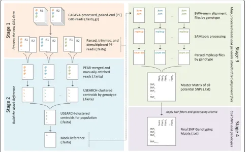
The GBS-SNP-CROP workflow
GBS-SNP-CROP, with particular emphasis on the rationale throughout. While the relevant Perl scripts are refer-enced in this discussion, please refer to the GBS-SNP-CROP User Manual for the details of pipeline execution (https://github.com/halelab/GBS-SNP-CROP.git).
Stage 1. Process the raw GBS data
As written, the code associated with Step 1 (“Parse the raw reads”; see Table 1) is compatible with Illumina1.8+ sequencing data, where the input files are assumed to be CASAVA-processed, paired-end (i.e. R1 and R2), and compressed FASTQ files (*.fastq.gz). As per the protocol developed by Poland et al. [11], these FASTQ files are assumed to contain multiplexed reads from a barcoded library of genotypes, where the R1 read begins with a 6– 10 bp barcode followed by the restriction site of the less-frequent cutter (e.g. PstI); and the R2 read begins with the restriction site of the more-frequent cutter (e.g.
MspI). To execute this stage of the pipeline, an auxiliary
text file is required that associates each barcode with its corresponding genotype ID (see example “Barcode-ID” file in Appendix A of the GBS-SNP-CROP User Manual).
The script for Step 1 processes the raw reads in a rela-tively standard manner, beginning by searching the R1 read for a high-confidence barcode sequence (i.e. no more than one mismatch, relative to the provided list of barcodes) immediately preceding the expected cut site remnant of the less frequent cutter. If both barcode and cut site are found, they are trimmed from the read, the barcode is appended to the headers of both the R1 and R2 reads, and the pair is retained for further processing. This first parsing script then searches for the 3′-ends of each GBS fragment, indicated by the in-line presence of the Illumina common adapter coupled with the appro-priate cut site residue. If found, the reads are truncated appropriately. Finally, all reads consisting of a majority of uncalled bases (i.e. N’s) are discarded.
Table 1Outline of the GBS-SNP-CROP workflow, featuring inputs and outputs of all seven steps (scripts)
Input file(s) Output file(s) Timea
(hrs:mins)
Stage 1. Process the raw GBS data
Step 1Parse the raw reads - CASAVA generated paired-end (R1, R2) files (.fastq.gz)
- Parsing summary information (.txt) 2:24
- Read length distribution summary (.txt)
- Barcode-ID file (.txt) - Parsed paired-end [PE] reads (.fastq)
- Parsed, unpaired R1 reads (.fastq)
Step 2Trim based on quality - Parsed PE reads (.fastq) - High quality, parsed PE reads (.fastq) 0:10
- High quality, parsed singletons (.fastq)
Step 3Demultiplex - One pair (R1, R2) of high quality files (.fastq) per library
- One pair (R1, R2) of high quality files (.fastq) per genotype
0:16
- Barcode-ID file (.txt)
Stage 2. Build the Mock Reference
Step 4Cluster reads and assemble the Mock Reference [MR]
- Genotype-specific PE files (.fastq) - Mock Reference [centroids] (.fasta) 0:14b
- Barcode-ID file (.txt) - Mock Reference [genome] (.fasta)
Stage 3. Map the processed reads and generate standardized alignment files
Step 5Align with BWA-mem and process with SAM tools
- Genotype-specific high quality PE files (.fastq)
- Filtered reads (.bam) 3:36
- Sorted BAM files (.sorted.bam)
- Reference or MR [genome] (.fasta) - Indexed BAM files (.sorted.bam.bai)
- Barcode-ID file (.txt) - Indexed reference or MR (.fasta.idx)
- One base call alignment summary file (.mpileup) per genotype
Step 6Parse mpileup output and produce the SNP discovery master matrix
- One base call alignment summary file (.mpileup) per genotype
- One base call alignment summary count file (.txt) per genotype
4:37
- Barcode-ID file (.txt) - SNP discovery master matrix (.txt)
Stage 4. Call SNPs and Genotypes
Step 7SNP genotyping across the population - SNP discovery master matrix (.txt) - SNP genotyping matrix for the population (.txt)
0:04
a
The computation times presented here are specific to the particular dataset in this study b
Further read trimming based on user-specified min-imums for both Phred quality score and read length is done in Step 2, using the bioinformatics tool Trimmo-matic [31]. Finally, in Step 3, all parsed and quality-filtered reads are processed according to their barcodes; and genotype-specific FASTQ files are produced for all genotypes. The final output of Stage 1 is a pair (R1 and R2) of FASTQ files for each genotype, containing all parsed and quality-filtered reads for downstream analysis.
Stage 2. Build the Mock Reference
If a suitable reference genome is available for the target population, one may move directly to Stage 3 of the pipeline. If such a reference is unavailable, however, the parsed and quality-filtered reads from Stage 1 are used to build a GBS-specific, reduced-representation refer-ence (hereafter “Mock Reference”) to enable GBS read mapping and facilitate SNP discovery. This stage of the pipeline relies upon a similarity-based clustering strategy to group the GBS reads, first within- and subsequently (if desired) across-genotypes, in order to generate repre-sentative reference sequences for the full set of GBS fragments.
To begin, the pipeline calls upon the PEAR software package [32] to merge the processed paired-end reads
into single reads spanning the complete GBS fragment lengths, wherever sequence overlap for a pair is suffi-cient (≥10 bp) to justify merging. For each genotype se-lected to contribute to the Mock Reference (see “ GBS-SNP-CROP Performance”), this step generates three different FASTQ files: An “assembled” file, containing successfully merged reads, and two “unassembled” files (R1 and R2), comprised of sequentially-paired R1 and R2 reads that could not be merged, due in part to a lack of sufficient overlap because of long GBS frag-ment lengths. Next, the pipeline stitches together all unmerged reads by joining pairs of sufficiently long
“unassembled” R1 and R2 sequences together with an intermediate run of 20 high-quality A’s, thus producing a FASTQ file of “stitched” R1 + R2 reads. Represent-ing the reduced genomic space targeted by the GBS restriction protocol, these PEAR-assembled and manually-stitched reads are then concatenated into a single FASTQ file per genotype for use in building the Mock Reference.
Next, GBS-SNP-CROP calls upon the USEARCH soft-ware package [33] to cluster these “assembled” and
“stitched” reads based on a user-specified similarity threshold, thereby producing a reduced list of non-redundant consensus sequences (centroids) that span the GBS fragment space. To accomplish this, the
USEARCH clustering procedure is executed first within
each selected genotype (i.e. USEARCH clusters “ assem-bled” and “stitched” reads into sets of genotype-specific centroids) and subsequently, if more than one genotype is selected to build the Mock Reference, across all se-lected genotypes (i.e. USEARCH clusters all genotype-specific centroids into a master set of centroids for the population). Representing the sampled GBS data space for the population, it is this resultant set of non-redundant consensus sequences that comprises the Mock Reference genome for subsequent mapping. De-pending on the intended use of the resultant genotypic data (e.g. diversity characterization, linkage map con-struction, trait association, etc.), the similarity threshold specified for USEARCH may be adjusted to collapse homologous regions or maximize their discrimination, an issue of particular relevance in polyploid species.
In the end, Stage 2 produces two different Mock Ref-erence FASTA files. The first (“MockRef_Genome.fasta”) consists of a single, long FASTA read comprised of all the centroids identified above, linked together into one contiguous sequence. The second (“ MockRef_Clusters.-fasta”) contains the same centroids in the same order, but in this case the centroid boundaries are preserved because each centroid exists as a separate FASTA entry. While the former file is used as the Mock Reference for read alignment (see next section), the latter is useful for optional downstream SNP filtering and analysis.
Stage 3. Map the processed reads and generate standardized alignment files
To align the processed reads from Stage 1 to the refer-ence, whether a true reference genome or a Mock Refer-ence built in Stage 2, GBS-SNP-CROP again relies upon familiar bioinformatics tools, in this case BWA [34] for alignment and SAMtools [35] for manipulating and pro-cessing the alignment output. Specifically, the BWA-mem algorithm is used to align the processed reads, genotype-by-genotype, to the reference. SAMtools is then called upon to accomplish the following steps: 1) Filter the mapped reads via SAMtools flags, retaining only those which map appropriately as pairs without po-tentially confounding secondary or supplementary align-ments (see the GBS-SNP-CROP User Manual for more detail); 2) Convert the filtered SAM files to BAM files; 3) Index and sort the BAM files; 4) Index the FASTA reference sequence; and 5) Produce a base call alignment summary (mpileup file) for each genotype. These six steps (BWA-mem alignment and the five SAMtools pro-cedures) are carried out individually for each genotype, with the Step 5 script automating the process.
In Step 6, the genotype-specific mpileup files are dis-tilled into“count”text files containing four essential tab-delimited columns: (1) Reference genome/chromosome
identifier; (2) Base position; (3) Reference base at that position; and (4) A comma-delimited string containing aggregated alignment information at that position (i.e. depths of A, C, G, and T reads). Each count file is then parsed, with only those rows containing reads poly-morphic to the reference sequence kept, thereby gener-ating liberal genotype-specific lists of potential SNP positions, with full read depth information retained. It is during this mpileup parsing that all putative indels are rigorously detected and excluded from downstream vari-ant calling, thus making GBS-CROP a SNP-exclusive pipeline.
Once the mpileup parsing is completed for each geno-type separately, Step 6 proceeds by mining the full set of resultant genotype-specific count files to generate a sin-gle, non-redundant master list of all potential SNP posi-tions throughout the target population. Alignment information is then extracted from the original count files for each genotype for all potential SNP positions in the master list and the data organized into a SNP discov-ery“master matrix”for the entire population. By capturing both genotype-specific (columns) and population-level (rows) alignment data in one table, the master matrix is a powerful and streamlined summary of the GBS data that contains the essential information to not only dis-tinguish high-confidence SNPs from likely sequencing and PCR errors but also to make subsequent genotype calls using stringent depth criteria, as explained in the next section.
Stage 4. Call SNPs and genotypes
Once generated, the master matrix is systematically pared down via a series of SNP-culling filters to arrive at a final “SNP genotyping matrix” containing only high-confidence SNPs and genotypes. To begin, the master list of potential SNPs is parsed based upon a flat criteria of independence, namely that a SNP is retained for further consideration if and only if there exist inde-pendent instances of the putative secondary allele, at a specified minimum depth (e.g. 3), across at least three genotypes. This simple requirement for independent occurrences of the less-frequent allele is an essential strategy for minimizing false SNP declarations due to random sequencing and PCR errors, including strand bias errors [36].
potential SNP is retained for further downstream ana-lysis if and only if it is strongly bi-allelic, that is if:
2oAllele Depth
2o
Depthþ3o
Depthþ 4o
Depth>altStrength
For a tetraploid species, we suggest a minimum value of 0.90 for this parameter, though higher values may be imposed in the interest of stricter error control (see Additional file 1).
After these initial basic population-level culling proce-dures, genotypic states (primary homozygote, heterozy-gote, or secondary homozygote) are assigned for all remaining SNP-accession combinations. To call a het-erozygote, a given genotype must have a user-specified minimum read depth for each allele (e.g. 3); and the read depth ratio of the lower-coverage to higher-coverage al-lele must exceed a user-specified, ploidy-appropriate threshold (e.g. 0.1; see Additional file 1). If the ratio falls below this minimum threshold, GBS-SNP-CROP re-frains from making a genotypic assignment (i.e. the genotype is designated as missing data). The GBS-SNP-CROP genotyping criterion for homozygotes is more stringent, requiring a relatively high, user-specified mini-mum depth (e.g.≥11 when the secondary allele count is zero and≥48 when the secondary allele count is one; see Additional file 1) in an effort to reduce the rate of erro-neous calls (i.e. true heterozygotes called as homozygous due to sampling bias). Finally, in an effort to retain only broadly informative SNPs, the matrix is further reduced such that all SNPs (i.e. rows) are discarded for which more than some user-specified maximum of genotypes are without genotypic calls, either because read depth = 0 or genotypic states were unassignable due to the cri-teria discussed above.
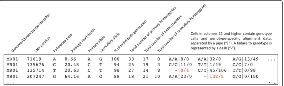
To facilitate the downstream characterization of the high-confidence SNPs that pass all the above filters, the
final SNP genotyping matrix contains both summary sta-tistics as well as complete genotype-specific alignment data for each retained SNP. As shown in Fig. 2, the first ten columns of the matrix feature the following informa-tion: 1) Genome/chromosome identifier; 2) SNP pos-ition; 3) Reference base; 4) Average read depth at that SNP position across the population; 5) Primary allele (i.e. the most frequent allele at that position, based on read depth across the population); 6) Secondary allele (i.e. the less frequent, or alternative, allele at that pos-ition); 7) Percentage of individuals from the population genotyped for that SNP; 8) Total number of homozy-gotes for the primary allele; 9) Total number of hetero-zygotes; and 10) Total number of homozygotes for the secondary allele. Columns 11 and higher contain the complete alignment data for each individual genotype for all possible SNP positions. The ability of GBS-SNP-CROP to consider both genotype-specific and population-level alignment data simultaneously through the master matrix during the processes of SNP filtering and genotyp-ing is an essential feature of the pipeline and motivates its disuse of Minor Allele Frequency (MAF), a problematic filtering parameter when attempting to characterize broadly diverse germplasm collections, as opposed to more closely-related breeding populations.
Other downstream tools
In addition to the scripts associated with the core GBS-SNP-CROP workflow described above, one additional script (“GBS-SNP-CROP-8.pl”) is provided to facilitate downstream management of the final SNP genotyping matrix by enabling users to convert the matrix into for-mats compatible with the familiar statistical analysis software packages R [37], Tassel GUI [30], and PLINK [38]. Specifically, the script produces a genotype matrix appropriate for diversity analyses within R (e.g. calculat-ing distance metrics, generatcalculat-ing cladograms, etc.) by
replacing primary homozygotes with 0, heterozygotes with 0.5, secondary homozygotes with 1, and unassigned genotypes with “NA”. It can also transform the final SNP genotyping matrix into a HapMap file for use as in-put into Tassel GUI, allowing users to easily access the functionality of that software package for forward ana-lysis, or create the transposed . PED file required by the whole genome association analysis toolset PLINK.
Avoiding false SNP calls
One well-recognized challenge posed by NGS data is the rate of erroneous base calls produced, rates which vary across both platforms and base position within reads. For instance, the error rate of current Illumina sequen-cing platforms ranges from 1 to 10 bases per kilobase se-quenced, with errors concentrated in the beginnings and ends of reads (i.e. tail distance bias) [39, 40]. With typ-ical sequencing runs producing billions of base calls (e.g. a single HiSeq 2500 Illumina flow cell can produce as much as 400 Gb of data [41]), there is real potential for millions of errors that can confound analysis [42]. Del Fabbro et al. [43] discuss the importance of quality trim-ming to increase the reliability of downstream analysis, with simultaneous gains in terms of both computational resources and time. While other authors assert that quality scores may not be perfectly reliable indicators of true nucleotide quality [44, 45], GBS-SNP-CROP begins with a stringent recognition of barcodes (Hamming dis-tance ≤1) and cut sites (no mismatches), followed by trimming based on Phred score.
In addition to this basic quality filtering of the raw reads, the pipeline seeks to minimize false SNP calls through its approach to SNP discovery and filtering. First, only those reads that map as paired-ends without secondary or supplementary alignments to the reference are retained. Additional parameters are called upon within the SAMtools mpileup algorithm to avoid false SNPs due to misalignment and excessive mismatches (see the GBS-SNP-CROP User Manual). SNPs that pass the above filters must then also satisfy the aforemen-tioned requirement of independence, assessable by virtue of the unique format of the GBS-SNP-CROP master matrix. By leveraging both genotype-specific and population-level depth information, this requirement ef-fectively reduces the probability of calling false SNPs due to both sequencing and PCR errors, including strand bias errors, since the exact same errors must arise independently, at depth, across multiple genotypes. GBS-SNP-CROP also makes use of stringent genotyping criteria to further reduce the probability of calling false SNPs and assigning incorrect genotypic states. Such genotyping criteria are based on relatively high depth re-quirements, information again accessible for evaluation via the master matrix.
Through its strict initial parsing and filtering of the raw reads as well as its rigorous approach to alignment, SNP filtering, and genotyping, GBS-SNP-CROP takes a very conservative approach to SNP calling. Nevertheless, as shown in the next section, the number of identified SNPs compares favorably to more permissive pipelines, in part because of GBS-SNP-CROP’s ability to make use of all available data, regardless of read length.
Finally, in addition to the embedded strategies for minimizing false SNP calls discussed here, users can eas-ily impose additional desired filters due to the fact that the output from all GBS-SNP-CROP steps, like the mas-ter matrix, are human-readable text files. For example, for the purpose of mapping studies as opposed to diver-sity analyses, which are the primary focus here, the elim-ination of markers in particularly SNP-dense regions may be an important quality control, as such high SNP density may be an artifact of promiscuous alignment, particularly in polyploids. In a reference-based approach, such culling is straightforward given the set of unique SNP coordinates across the linkage groups. In a reference-independent pipeline, a similar filter can be applied; but users will need to consider SNP densities within each cluster (centroid) used to build the Mock reference. To accomplish this, centroid boundaries must be located within the Mock Reference, which is one rea-son why the second Mock Reference (clusters) file is generated by the pipeline, to enable such projection.
GBS-SNP-CROP performance
We assessed the performance of GBS-SNP-CROP in genotyping a population of 48 diverse accessions of the perennial dioecious tetraploid Actinidia arguta. Specific-ally, its performance using both a reference from a related diploid species (A. chinensis) and a Mock Reference was compared to that of TASSEL-GBS [30], a widely-used reference-based pipeline, and TASSEL-UNEAK [15], its reference-independent version.
Sampling strategy to build a Mock Reference
scenarios where fewer genotypes were used to construct the Mock Reference, first using only the top five geno-types (ranked simply by the number of parsed reads) and then again using only the top genotype. Using the five genotypes with the highest numbers of parsed reads, the pipeline assembled the Mock Reference in less than an hour and identified 20,226 potential SNPs (average depth = 71.0). Using only the single most read-abundant genotype, the pipeline assembled the Mock Reference in 14 min and called 21,318 SNPs (average depth = 69.3). Based on these results, all subsequent pipeline evalu-ation was conducted using the results from GBS-SNP-CROP-MR01 (i.e. Mock Reference constructed from one genotype). The pipeline itself is flexible, however, able to integrate centroids from multiple genotypes into a Mock
Reference, a feature of potential use for genotyping par-ticularly diverse populations (e.g. multiple closely-related species).
Data usage
One of the most noteworthy differences between the GBS-SNP-CROP and TASSEL pipelines is the ability of GBS-SNP-CROP to access and make use of a greater amount of sequence data (Table 3). In the TASSEL-GBS pipeline, due to its tag-based alignment strategy, a uni-form tag length (mxTagL) must be specified that effect-ively limits the number of reads used for analysis. According to the TASSEL 5.2.11 manual, “the mxTagL value must be chosen such that the longest barcode + mxTagL < read length” [30]; thus all reads that violate
Table 2Performance of GBS-SNP-CROP under three different sampling strategies for building the Mock Reference: Using all 48 individuals in the population (MR48), using only the 5 individuals with the highest number of parsed reads (MR05), and using only the single most read-abundant genotype (MR01)
Pipelines Total number of centroids used to build the Mock Referencea
Total number of paired-end reads used for SNP callingb
Number of
SNPs calledc Avg. depth d
Hetero (%)e Homo (%)f Missing
data (%)g Time(hrs:mins)h
GBS-SNP-CROP-MR48 1,276,734 92,667,123 14,712 70.74 32.47 59.31 8.20 14:30
GBS-SNP-CROP-MR05 500,795 132,920,383 20,226 71.02 34.50 57.18 8.31 12:06
GBS-SNP-CROP-MR01 229,549 154,506,669 21,318 69.34 34.51 56.85 8.29 11:03
a
Total number of non-redundant consensus sequences (centroids) identified via clustering to represent the GBS fragment space. This is also the number of FASTA entries in the“MockRef_Clusters.fasta”file
b
Number of reads retained by the pipeline after mapping procedures and thus used for SNP calling c
Total number of SNPs called, given all SNP calling filters and genotyping criteria described in the text d
Average read depth for all SNPs across the entire population e
Percentage of heterozygous genotype calls f
Percentage of homozygous genotype calls g
Percentage of missing cells (i.e. no genotype call for a given SNP*accession combination) in the final SNP genotype matrix h
The total computation time required for all pipeline analysis when executed on a Unix workstation with 16 GB RAM and a 2.6 GHz Dual Intel processor
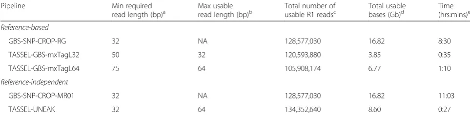
Table 3Comparative data usage and computation times for five different analyses of 150 bp paired-end GBS data from 48 accessions
ofActinidia arguta
Pipeline Min required
read length (bp)a
Max usable read length (bp)b
Total number of usable R1 readsc
Total usable bases (Gb)d
Time (hrs:mins)e
Reference-based
GBS-SNP-CROP-RG 32 NA 128,577,030 16.82 8:30
TASSEL-GBS-mxTagL32 50 32 120,593,880 3.85 0:35
TASSEL-GBS-mxTagL64 75 64 105,908,174 6.77 1:10
Reference-independent
GBS-SNP-CROP-MR01 32 NA 128,577,030 16.82 11:03
TASSEL-UNEAK 32 64 134,352,640 8.60 0:27
a
GBS-SNP-CROP utilizes the entire R1 and R2 paired-end sequences of all parsed and quality trimmed reads longer than a user-specified (i.e. adjustable) minimum length, in this case 32 bp. The TASSEL-GBS pipelines utilize a uniform user-specified portion (e.g. 32 bp, 64 bp) from the beginning of acceptable R1 (single-end) reads that exceed a minimum length (e.g. 50 bp, 75 bp) before barcode and cut site trimming. TASSEL-UNEAK utilizes up to 64 bp from the beginning of accept-able R1 (single-end) reads that exceed a minimum length of 32 bp after barcode and cut site trimming
b
The maximum length of sequences utilized by GBS-SNP-CROP is set by the sequencing platform (e.g. 100 bp, 150 bp, etc.). In TASSEL-GBS, the user specifies a maximum tag length, thereby effectively setting a uniform tag length. The maximum usable sequence length in TASSEL-UNEAK is 64 bp, with all shorter reads greater than 32 bp padded with poly-A’s to a uniform 64 bp tag length
c
The number of R1 (i.e. single-end) reads ultimately used by each pipeline, after filtering based on quality and read length requirements. The R1 (single-end) counts are shown here to facilitate comparison across pipelines. Because GBS-SNP-CROP utilizes paired-end reads, the total number of actual reads used (R1 and R2) is twice this number
d
The total number of nucleotides of sequence data used in each analysis e
this statement are discarded. Further, all reads that meet this requirement are subsequently truncated to a uniform length based on this parameter; thus not only short reads but also the full lengths of long reads are culled. While this tag length requirement is adjustable within TASSEL-GBS (here, we ran the pipeline with tag lengths of both 32 bp as well as the default 64 bp), it is fixed at 64 bp for TASSEL-UNEAK. In contrast, aside from a user-specified minimum read length, GBS-SNP-CROP imposes no requirement for read length uniformity, even within read pairs.
Following initial parsing and quality trimming (Stage 1), a total of 16.82 Gb of sequence data was found to be us-able for analysis (alignment, SNP discovery, etc.) within GBS-SNP-CROP (Table 3). In contrast, due mainly to tag length requirements and the usability of only R1 (single-end) reads, a much reduced 3.85 Gb, 6.77 Gb and 8.60 Gb were used, respectively, by the TASSEL-GBS (mxTagL = 32), TASSEL-TASSEL-GBS (mxTagL = 64) and TASSEL-UNEAK pipelines. In terms of data usage, therefore, GBS-SNP-CROP performs quite favorably, with approximately 2.0–4.4 times more high-quality se-quence data available to it for SNP discovery.
In theory, one should be able to make more reads available to TASSEL-GBS by reducing the mxTagL threshold. Such a reduction (in this case, from 64 to 32 bp) leads, however, to a significant reduction in over-all data usage (from 6.77 Gb to 3.85 Gb; Table 3) and a concomitant reduction in identified SNPs (from 8,907 to
5,593; Table 4B). For TASSEL-GBS, therefore, it may be advantageous to set a larger mxTagL value, thereby dis-carding a larger number of reads that fail to meet that requirement, than to use a higher number of shorter reads permitted by a lower mxTagL value.
The low average proportion (10.8 %) of shared SNPs discovered by TASSEL-GBS under both the 32 and 64 bp mxTagL scenarios (Fig. 3; Additional file 2) indi-cates that essentially different datasets are made avail-able to the TASSEL-GBS pipeline, depending on the chosen value of this one parameter. Such a comparison suggests that the requirement within the TASSEL pipe-lines for uniform read lengths (i.e. TASSEL’s tag-based mapping strategy) is fundamentally limiting, in terms of data usage. By taking a read-based rather than a tag-based approach to alignment and SNP discovery, GBS-SNP-CROP leverages all available data in a single analysis, thereby avoiding undue fractionation of the dataset.
Numbers of SNPs
Analyses by the different pipelines lead to widely varying numbers of identified SNPs (Table 4). Using only the single most read-abundant genotype to build the Mock Reference, GBS-SNP-CROP called 56,598 potential SNPs (average depth = 44.5; Table 4A), of which 21,318 were retained after applying all SNP calling and genotyping filters (Table 4B), a reduction of 62.3 %. In comparison, the reference-free TASSEL-UNEAK pipeline called
Table 4Comparative pipeline performances before (4A) and after (4B) depth-based genotyping criteria and population-level SNP calling filters for 150 bp paired-end GBS data from 48 accessions ofActinidia arguta
Pipeline Number of SNPsa Average depth [D]b Reads with D
≥20 (%)c Hetero (%)d Homo (%)e Missing data (%)f
4A. No SNP calling or genotyping filters appliedg
GBS-SNP-CROP-MR01 56,598 44.47 52.85 26.19 57.25 16.55
GBS-SNP-CROP-RG 23,564 47.39 39.00 26.10 51.09 22.80
TASSEL-UNEAK 12,905 6.98 9.61 13.93 52.12 33.94
TASSEL-GBS-mxTagL32 19,095 134.18 49.20 16.86 71.66 11.46
TASSEL-GBS-mxTagL64 25,005 34.65 35.60 19.21 65.80 14.98
4B. Depth-based genotyping criteria and population-level SNP calling filters appliedh
GBS-SNP-CROP-MR01 21,318 69.34 99.92 34.51 56.85 8.64
GBS-SNP-CROP-RG 5,471 77.11 99.85 38.31 53.29 8.40
TASSEL-UNEAK 1,160 44.70 83.62 31.66 66.61 1.73
TASSEL-GBS-mxTagL32 5,593 64.41 92.52 26.33 71.58 2.09
TASSEL-GBS-mxTagL64 8,907 51.42 78.07 27.80 69.36 2.84
a
Total number of SNPs called within each pipeline, under the indicated SNP calling filters and genotyping criteria b
Average read depth for all SNPs across the entire population c
Percentage of called SNPs with an average read depth of at least 20 d
Percentage of heterozygous genotype calls e
Percentage of homozygous genotype calls f
Percentage of missing cells (i.e. no genotype call for a given SNP*accession combination) g
Liberal pipeline results in the absence of subsequent SNP calling or genotyping filters h
12,905 potential SNPs (average read depth = 7.0), of which only 1,160 SNPs passed these same filters, a strik-ing reduction of 91.0 %.
Using the published A. chinensisdiploid genome as a reference and a liberal pipeline (i.e. no imposed SNP cul-ling or genotyping filters), GBS-SNP-CROP-RG called 23,564 potential SNPs (average depth = 47.4), of which 5,471 were retained after filtering, a reduction of 76.8 %. In comparison, the 32 and 64 bp reference-based TASSEL-GBS analyses called 19,095 and 25,005 potential SNPs (average depths of 134.2 and 34.7, respectively), of which 5,593 (70.7 % reduction) and 8,907 (64.4 % reduc-tion) passed the imposed filters (Table 4). Unlike the reference-independent analyses, therefore, TASSEL-GBS was found to outperform the reference-based GBS-SNP-CROP in terms of numbers of identified SNPs.
Using only those SNPs that passed the stringent geno-typing criteria and population-level filters described earl-ier, we compared the set of SNPs called by GBS-SNP-CROP (using the A. chinensis reference) with those called by the TASSEL-GBS analyses (Table 4B). There is strikingly little congruence among these analyses, with many unshared markers (on average 96.3 %) between them (Fig. 3; Additional file 2). Interestingly, a high pro-portion of unshared markers (on average 89.2 %) also exists between the two different TASSEL-GBS analyses themselves, even though they differ only in their speci-fied mxTagL thresholds. Because the initial dataset is the same for both TASSEL analyses, we expected roughly half of the SNPs called under mxTagL = 64 to also be called under mxTagL = 32 (i.e. that SNPs located within the first 32 bases of the mxTagL = 64 SNPs should com-prise a proportional subset of the mxTagL = 32 SNPs); but such is not the case (see Fig. 3).
One stated reason for TASSEL’s approach to SNP call-ing based on tags is decreased computational time spent for pipeline execution, with the added rationale that se-quencing errors increase after the first 64 bp of a read [11, 30]. While this may be the case, TASSEL’s SNP dis-covery method appears to be highly sensitive to this tag length parameter, a result that suggests there may be some benefit in aggregating the results (i.e. lists of SNPs) of multiple TASSEL-GBS analyses under various mxTagL values. Similarly, the largely non-overlapping re-sults of the reference-based GBS-SNP-CROP analysis may also have value as a complement to the TASSEL-GBS approach.
To investigate the overlap among the sets of SNPs called between the based and reference-independent pipelines, we mapped all SNPs discovered using both GBS-SNP-CROP (Mock Reference centroids) and TASSEL-UNEAK (tags) to the A. chinensis refer-ence. In so doing, we found that 33.7 % of the SNPs called by the reference-based GBS-SNP-CROP (A. chi-nensis) were also called by the reference-independent GBS-SNP-CROP (Mock Reference based on the single most read-abundant genotype). In contrast, only 0.6 and 0.4 % of the SNPs called by TASSEL-GBS (64 and 32 bp, respectively) were identified by the reference-independent TASSEL-UNEAK pipeline (Fig. 3; Additional file 2).
Average depth
One of the most efficient means of distinguishing se-quencing error from true nucleotide polymorphism is to increase read depth thresholds because polymorphisms called on the basis of more reads mapped to the same locus can be declared with greater reliability that those based on fewer reads [46]. Nielsen et al. [47] discussed
many studies using NGS data with medium-to-low coverage (<20×) and showed that genotype calls based on such data exhibit statistical uncertainty. According to the authors, there are two reasons for this: (1) In hetero-zygotes, both alleles may not be sampled, thus leading to incorrect homozygote calls; and (2) In the case of high sequencing error technologies, a significant number of homozygotes may be incorrectly declared heterozygotes if genotype calling is based simply on the allelic pres-ence/absence. According to Illumina’s technical notes [35], the probability of making a correct genotyping call is roughly 95 % for 20× coverage. While 99.9 % of the 21,318 SNPs identified by the GBS-SNP-CROP Mock Reference pipeline have an average read depth higher than 20×, this is true of only 83.6 % of the 1,160 SNPs called by TASSEL-UNEAK (Table 4). In comparison, 92.5 % of the 5,593 SNPs (-mxTagL32) and 78.1 % of the 8,907 SNPs (-mxTagL64) called by the reference-based TASSEL-GBS pipelines have an average read depth higher than 20×, compared to 99.9 % of the 5,471 SNPs called by the reference-based GBS-SNP-CROP. In terms of average read-depth, therefore, GBS-SNP-CROP per-forms favorably compared to both TASSEL-GBS and TASSEL-UNEAK (see Additional file 3).
Recognizing biological replicates
The primary motivation for developing GBS-SNP-CROP was the need for a tool to accurately characterize the genetic diversity of understudied germplasm collections, including identifying redundant accessions as a means of boosting the resource efficiency of curation efforts. Given this goal, a relevant performance criterion is the ability of the pipeline to identify biological replicates in a population, as indicated by the observed genetic distance between those replicates. To quantify such distance, we employed a modified Gower’s Coefficient of Similarity [48], ranging from 0 to 1, to quantify identity-by-state based on bi-allelic SNPs:
SGowerðx;yÞ ¼
Xm i¼1siwi
Xm i¼1wi
where si= 1 if the genotypes are the same, 0.5 if the
genotypes differ by one allele (i.e. heterozygote vs. homozygote), and 0 if the genotypes differ by both al-leles (i.e. primary homozygote vs. secondary homozy-gote); and wi= 1 if both replicates are genotyped for the
SNP in question and 0 if either replicate lacks an assigned genotypic state.
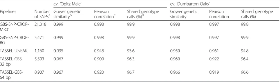
Using the SNPs called by the GBS-SNP-CROP-MR01 analysis (Table 4B), the Gower genetic similarity calcu-lated between two biological replicates of A. arguta ac-cession ‘Opitz Male’ was found to be 0.999, with a Pearson correlation of 0.998, results similar to those
obtained with the reference-based GBS-SNP-CROP pipeline (Table 5). In comparison, the reference-based TASSEL-GBS-32 bp and -64 bp analyses yielded lower Gower genetic similarities of 0.967, as well as reduced Pearson correlations (≤ 0.92). These same replicates of
’Opitz Male’ were found to be only 0.948 similar by TASSEL-UNEAK, indicating a genotyping error rate of more than 60 times that of GBS-SNP-CROP (Mock Ref-erence), despite calling 18 times fewer SNPs (1,160 vs. 21,318; Table 4B). This same basic pattern of results was found when analyzing biological replicates of A. arguta
accession ‘Dumbarton Oaks’ (Table 5), suggesting that genotyping via GBS-SNP-CROP is relatively robust, prone to fewer genotyping errors while maintaining high numbers of SNPs, whether or not a reference is available.
Computation time
Compared to TASSEL-UNEAK, the GBS-SNP-CROP Mock Reference workflow processed over twice as much data, generated over 18 times more SNPs, the SNPs it called had higher average depth (69.3 vs. 44.7), and as a set they were better able to detect similarity between biological replicates; but this improved performance comes at the price of approximately 25 times longer computation time. Using a dedicated Unix workstation with a 2.6 GHz Dual Intel processor and 16 GB RAM, the computational time required to run the Mock Refer-ence GBS-SNP-CROP pipeline using only the most read-abundant genotype to assemble the Mock Refer-ence was approximately 11 h for this dataset, compared to only 27 min for the TASSEL-UNEAK analysis (Table 2). Similarly, due to its consideration of 3–4 times the amount of sequence data and its strategy of mapping reads rather than tags, the reference-based GBS-SNP-CROP analysis (~8.5 h) also requires significantly more computational time than either of the TASSEL-GBS ana-lyses (35–70 min). Table 1 presents the computational times required for each of the steps within the reference-free GBS-SNP-CROP-MR01 workflow.
Conclusions
evolutionary ecology, conservation biology, and genetic linkage analysis.
As indicated by the example analysis presented here, the pipeline performs quite favorably compared to TASSEL-UNEAK, not only in terms of a significantly higher number of identified SNPs but also in terms of an increased average read depth and a greatly reduced genotyping error rate. Remarkably, the reference-independent version of GBS-SNP-CROP was also shown to outperform the reference-based TASSEL-GBS pipe-line in terms of these same metrics. In contrast, the reference-based version of GBS-SNP-CROP appears out-performed by TASSEL-GBS in terms of the number of called SNPs, though again its genotyping error rate is lower. Given the low proportion of shared SNPs among these reference-based analyses, however, GBS-SNP-CROP may be useful even in this case, able to detect large numbers of additional high-quality SNPs missed by the tag-based and read length-restricted approach of TASSEL-GBS. Indeed, with the capacity to make full use of variable length, paired-end GBS data for high-density SNP genotyping of plant populations, whether or not a reference genome is available, GBS-SNP-CROP is a flex-ible and easily modifiable tool worthy of consideration by interested programs.
Methods
Plant material, GBS data, and genotypes sampled
A collection of 48 tetraploid kiwiberry (Actinidia arguta) genotypes, each carrying two sets of 29 chromosomes (2n = 4× = 116) with an estimated total genome size of 1C = 1.5 Gbp [49], was sampled from the USDA Na-tional Clonal Germplasm Repository (Davis, CA) for this study. Genomic DNA was extracted from ~1 g of fresh young leaves from each accession using a modified CTAB protocol, and a multiplexed GBS library was pre-pared according to the two enzyme (PstI-MspI) protocol
described by Poland et al. [11]. Using the first 96 6– 10 bp barcodes from that protocol, the 48 accessions were multiplexed along with 2 biological replicates (accessions “Opitz Male” and “Dumbarton Oaks”) and 46 breeding lines, resulting in a 96-plex library which was sequenced on two lanes (i.e. one complete flowcell) of an Illumina 2500 HiSeq machine at the Hubbard Center for Genome Studies, University of New Hampshire (http://hcgs.unh.edu/). FASTQ files of the sequence data were generated using CASAVA 1.8.3 [50]; and these raw sequences have been deposited in the NCBI Sequence Read Archive (SRA Accession number SRR2296676). A table of the 48 genotypes used in this analysis, along with their assigned barcodes, can be found in Additional file 4.
Pipeline evaluation and testing
To evaluate the performance of GBS-SNP-CROP, we an-alyzed the GBS data from the 48 accessions described above (plus 2 biological replicates) using seven different analyses. First, we executed three variations of GBS-SNP-CROP without a reference genome (Table 1, Stage 2). In the first Mock Reference analysis (GBS-SNP-CROP-MR48), we assembled the Mock Reference from centroids identified by clustering first within each geno-type and then across all 48 genogeno-types in the population. In the second Mock Reference analysis (GBS-SNP-CROP-MR05), clustering was done across only the five most read-abundant genotypes (accessions“ORUS 2–16”,
“DACT 213”, “40537C”, “ORUS 1–6”, and “Chang Bai Mountain 3”). In the third analysis (GBS-SNP-CROP-MR01), the Mock Reference was built using the within-genotype centroids from only the single most read-abundant line (accession “ORUS 2–16”). These three different approaches were followed to examine the effects of reducing the number of genotypes used to build the Mock Reference on both computational time and the number and quality of identified SNPs.
Table 5Comparative pipeline performances, in terms of consistency in genotyping biological replicates
cv.‘Opitz Male’ cv.‘Dumbarton Oaks’
Pipelines Number
of SNPsa Gower geneticsimilarityb Pearsoncorrelationc Shared genotypecalls (%)d Gower geneticsimilarity Pearsoncorrelation Shared genotypecalls (%)
GBS-SNP-CROP-MR01
21,318 0.999 0.998 99.9 0.998 0.997 99.8
GBS-SNP-CROP-RG
5,471 0.999 0.998 99.9 0.998 0.997 99.9
TASSEL-UNEAK 1,160 0.935 0.948 93.6 0.950 0.961 94.8
TASSEL-GBS-32 bp
5,593 0.967 0.909 96.3 0.969 0.922 96.4
TASSEL-GBS-64 bp
8,907 0.967 0.920 96.7 0.966 0.919 96.6
a
The total number of SNPs used in this analysis refers to numbers from Table4B b
A modified Gower’s general Coefficient of Similarity [48], ranging from 0 to 1, to quantify identity-by-state based on bi-allelic SNPs c
Pearson correlation calculated using R [31]; for all correlations in the table,p-value< 0.01 d
For all Mock Reference analyses, we used PEAR v.0.96 [32] to merge reads using mainly default parameters, except for specifying a minimum assembled read length of 32 bp. For clustering, we used USEARCH v.8.0.162 [33], specifying the “cluster_fast” algorithm with a nucleotide similarity threshold of 93 % to allow up to two mis-matches within the shortest assembled reads (32 bp).
For comparison with the Mock Reference analyses de-scribed above, we ran GBS-SNP-CROP using a pub-lished reference genome from the closely related diploid (2n = 2× = 58) speciesA. chinensis[51] with an estimated genome size 1C = 758 Mbp [48]. The only difference be-tween this reference-based analysis (GBS-SNP-CROP-RG) and the Mock Reference analyses above is that in the former we skipped Stage 2 (“Build the Mock Refer-ence”) of the GBS-SNP-CROP workflow (see Table 1).
For both GBS-SNP-CROP analyses, the CASAVA-processed sequence data were subjected to basic quality filtering. Specifically, reads were trimmed based on a sequence of three contiguous bases with an average Phred score Q ≤30, and trimmed reads shorter than 32 bp were culled. These procedures were performed using the Trimmomatic software v.0.33 [31] with the following parameters: LEADING:30 SLIDINGWIN-DOW:4:30 TRAILING:30 MINLEN:32. Also for both analyses, alignment was carried out using BWA v.0.7.12 [34]; and the resultant alignment files were processed with SAMtools v.1.2 [35].
For the next analysis, we used the Network-Based SNP Discovery Protocol with no reference genome (TASSEL-UNEAK v.3.0). The TASSEL-(TASSEL-UNEAK pipeline was run using mainly its default parameters, with two changes: (1) In the “UMergeTaxaTagCountPlugin” step, the “-c” flag was increased from 5 to 10; and (2) The error toler-ance rate (“-e” flag on “UTagCountToTagPairPlugin”) was decreased from 0.03 to 0.01. These modifications were made in an effort to match the default parameters of the TASSEL-GBS analyses, thereby facilitating comparison.
Finally, we used TASSEL-GBS v.5.2.11 to carry out two more reference-based analyses, one with“Maximum Tag Length” (mxTagL) = 32 bp and the other with mxTagL = 64 bp. For all TASSEL analyses (TASSEL-GBS-32 bp, TASSEL-GBS-64 bp, and TASSEL-UNEAK), we set the minimum minor allele frequency to 5 % and accepted only those markers for which genotypes were called for at least 75 % of the population.
Comparing called SNPs among pipelines
Identifying shared and non-shared SNPs called by the reference-based pipelines (GBS-SNP-CROP-RG and the TASSEL-GBS pipelines) is straightforward due to the unique coordinate positions of the SNPs within the
common A. chinensis reference genome. Comparing called SNPs between the reference-independent pipelines (TASSEL-UNEAK and GBS-SNP-CROP-MR01) and reference-based pipelines is less simple due to the fact that no common reference (and thus coordinate system) exists. To enable such important comparisons, we first located the positions of all called SNPs (Table 4B) within the indi-vidual centroids used to construct the Mock Reference (GBS-SNP-CROP-MR01) and within the unique 64 bp tags used within the TASSEL-UNEAK pipeline. We then mapped all the putative SNP-containing centroids/tags to theA. chinensisreference genome and located the corre-sponding A. chinensis coordinate position of each called SNP. Finally, the allele compositions of any supposedly common SNPs were verified before such SNPs were de-clared as shared between pipelines.
Availability of supporting data
The data set supporting the results of this article is avail-able in the NCBI Sequence Read Archive [SRA Accession number SRR2296676].
Additional files
Additional file 1:Suggested parameter values for GBS-SNP-CROP, based on ploidy scenarios and confidence considerations. AdditionalFile1.pdfpresents rationale to guide user selection of ploidy-appropriate values for various parameters in Script 7 of GBS-SNP-CROP (-mnHoDepth0, -mnHoDepth1, -mnAlleleRatio, and–altStrength). (PDF 1231 kb)
Additional file 2:Bubble plot showing the pair-wise percentage of
shared markers called by the different pipelines.AdditionalFile2.pdf
complements the visualization in Fig. 3, showing all pair-wise proportions of shared SNPs among the five evaluated pipelines. (PDF 732 kb)
Additional file 3:The distribution of pre-filtered SNPs across three
different depth classes: Low (<4), Acceptable (4–200), and
Over-represented (>200).The bar plot inAdditionalFile3.pdfcompares the
distributions of average read depths for the pre-filtered SNPs called by the five evaluated pipelines. (PDF 43 kb)
Additional file 4:List of the 48A. argutagenotypes used for
GBS-SNP-CROP development and analysis.AdditionalFile4.pdfpresents
the names of the genotypes from the USDA National Clonal Germplasm Repository used in this study, along with their barcodes and the number of parsed GBS reads obtained for each. (PDF 50 kb)
Competing interests
The authors declare they have no competing interests.
Authors’contributions
All authors contributed to the development, troubleshooting, and improvement of the pipeline. AM conducted the comparative pipeline analyses and performance evaluations. AM and IH developed the manuscript. IH coordinated and contributed to all aspects of the work. All authors have read and approved the final manuscript.
Acknowledgements
Author details
1College of Life Sciences and Agriculture, Department of Biological Sciences,
University of New Hampshire, Durham, NH, USA.2College of Life Sciences
and Agriculture, Genetics Graduate Program, University of New Hampshire, Durham, NH, USA.
Received: 8 September 2015 Accepted: 6 January 2016
References
1. McCouch S, Baute GJ, Bradeen J, Bramel P, Bretting PK, Buckler E, et al. Agriculture: Feeding the future. Nature. 2013;499:23–4.
2. Tester M, Langridge P. Breeding technologies to increase crop production in a changing world. Science. 2010;327:818–22.
3. Godfray HCJ, Beddington JR, Crute IR, Haddad L, Lawrence D, Muir JF. Food Security: The Challenge of Feeding 9 Billion People. Science. 2010;327:812–8.
4. Naylor RL, Falcona WP, Goodmanb RM, Jahnc MM, Sengoobad T, Teferae H, et al. Biotechnology in the developing world: a case for increased investments in orphan crops. Food Policy. 2004;29(1):15–44.
5. Mayes S, Massawe FJ, Alderson PG, Roberts JA, Azam-Ali SN, Hermann M. The potential for underutilized crops to improve security of food production. J Exp Bot. 2011;63(3):1075–9. doi:10.1093/jxb/err396. 6. Kennedy G, Nantel G, Shetty P. The scourge of hidden hunger: global
dimensions of micronutrient deficiencies. Food Nutrition and Agriculture. 2003;32:8–16.
7. Tadele Z. Role of orphan crops in enhancing and diversifying food production in Africa. African Technology Development Forum Journal. 2009;6(3):9–15.
8. Altieri MA, Funes-Monzote FR, Petersen P. Agroecologically efficient agricultural systems for smallholder farmers: contributions to food sovereignty. Agron Sustain Dev. 2012;32(1):1–13.
9. Pérez-de-Castro AM, Vilanova S, Cañizares J, Pascual L, Blanca LM, Díez MJ, et al. Application of Genomic Tools in Plant Breeding. Curr Genomics. 2012;13(3):179–95.
10. Elshire RJ, Glaubitz JC, Sun Q, Poland JA, Kawamoto K, Buckler ES, et al. A robust, simple Genotyping-by-Sequencing (GBS) approach for high diversity species. PLoS One. 2011;6(5):e19379. doi:10.1371/journal.pone.0019379. 11. Poland JA, Brown PJ, Sorrells ME, Jannink JL. Development of high-density
genetic maps for barley and wheat using a novel two-enzyme Genotyping-by- Sequencing approach. PLoS One. 2012;7(2):e32253. doi:10.1371/journal. pone.0032253.
12. Poland JA, Rif TW. Genotyping-by-Sequencing for Plant Breeding and Genetics. Plant Genome. 2012;5:92–102.
13. Poland JA, Endelman J, Dawson J, Rutkoski J, Wu S, Manes Y, et al. Genomic Selection in Wheat Breeding using Genotyping-by-Sequencing. The Plant Genome. 2012;5:103–13.
14. Peterson GW, Dong Y, Horbach C, Fu YB. Genotyping-By-Sequencing for Plant Genetic Diversity Analysis: A Lab Guide for SNP Genotyping. Diversity. 2014;6(4):665–80.
15. Lu F, Lipka AE, Glaubitz J, Elshire R, Cherney JH, Cherney JH, et al. Switchgrass genomic diversity, ploidy, and evolution: novel insights from a network-based SNP discovery protocol. PLoS Genet. 2013;9(1):e1003215. doi:10.1371/journal.pgen.1003215.
16. Fu YB, Cheng B, Peterson GW. Genetic diversity analysis of yellow mustard (Sinapis albaL.) germplasm based on genotyping by sequencing. Genetic Resource Crop Evolution. 2014;61:579–94.
17. Lombardi M, Materne M, Cogan NOI, Rodda M, Daetwyler HD, Slater AT, et al. Assessment of genetic variation within a global collection of lentil (Lens culinarisMedik.) cultivars and landraces using SNP markers. BMC Genet. 2014;15:150. doi:10.1186/s12863-014-0150-3.
18. Wang B, Tan HW, Fang W, Meinhardt LW, Mischke S, Matsumoto T, et al. Developing single nucleotide polymorphism (SNP) markers from transcriptome sequences for identification of longan (Dimocarpus longan) Germplasm. Horticulture Research. 2015;2:14065. doi:10.1038/hortres.2014.65. 19. Cabezas JA, Ibanez I, Lijavetzky D, Velez D, Bravo G, Rodriguez V, et al. A 48
SNP set for grapevine cultivar identification. MC Plant Biology. 2011;11:153. 20. Wu B, Zhong GY, Yue JQ, Yang RT, Li C, Li YJ, et al. Identification of
Pummelo Cultivars by Using a Panel of 25 Selected SNPs and 12 DNA Segments. PLoS One. 2014;9(4):e94506. doi:10.1371/journal.pone.0094506.
21. Wong MML, Verma NG, Ramsay L, Yuan HY, Caron C, Diapari M, et al. Classification and Characterization of Species within the Genus Lens Using Genotyping-by-Sequencing (GBS). PLoS One. 2015;10(3):e0122025. doi:10.1371/journal.pone.0122025.
22. Narum SR, Buerkle CA, Davey JW, Miller MR, Hohenlohe PA. Genotyping-by-sequencing in ecological and conservation genomics. Mol Ecol. 2013;22(11):2841–7.
23. Leggett RM, MacLean D. Reference-free SNP detection: dealing with the data deluge. BMC Genomics. 2014;15(4):S10.
24. Kumar S, Banks TW, Cloutier S. SNP Discovery through Next-Generation Sequencing and Its Applications. International Journal of Plant Genomics. 2012;2012:831460. doi:10.1155/2012/831460.
25. Varshney RK, Ribaut JM, Buckler ES, Tuberosa R, Rafalski JA, Langridge P. Can genomics boost productivity of orphan crops? Nat Biotechnol. 2012;30:1172–6.
26. African Orphan Crops Consortium (AOCC). http://africanorphancrops.org (2015). Accessed 30 Aug 2015.
27. Maranz S, Kpikpi W, Wiesman Z, Sauveur ADS, Chapagain B. Nutritional values and indigenous preferences for Shea Fruits (Vitellaria paradoxaC.F. Gaertn. F.) in African Agroforestry Parklands. Econ Bot. 2004;58(4):588–600. 28. Maranz S, Niang A, Kalinganire A, Konaté D, Kaya B. Potential to harness
superior nutritional qualities of exotic baobabs if local adaptation can be conferred through grafting. Agrofor Syst. 2008;72(3):231–9.
29. Weerahewaa J, Rajapakseb C, Pushpakumarac G. An analysis of consumer demand for fruits in Sri Lanka 1981–2010. Appetite. 2013;60:252–8. 30. Glaubitz JC, Casstevens TM, Lu F, Harriman J, Elshire RJ, Sun Q, et al.
TASSEL-GBS: A High Capacity Genotyping by Sequencing Analysis Pipeline. PLoS One. 2014;9(2):e90346. doi:10.1371/journal.pone.0090346.
31. Bolger AM, Lohse M, Usadel B. Trimmomatic: A flexible trimmer for Illumina Sequence Data. Bioinformatics. 2014;30(15):2114–20.
32. Zhang J, Kobert K, Flouri T, Stamatakis A. PEAR: a fast and accurate Illumina Paired-End reAd mergeR. Bioinformatics. 2014;30(5):614–20.
33. Edgar RC. Search and clustering orders of magnitude faster than BLAST. Bioinformatics. 2010;26(19):2460–1.
34. Li H, Durbin R. Fast and accurate short read alignment with Burrows-Wheeler Transform. Bioinformatics. 2009;25:1754–60.
35. Li H, Handsaker B, Wysoker A, Fennell T, Ruan J, Homer J, et al. The Sequence Alignment/Map format and SAMtools. Bioinformatics. 2009;25(16):2078–9.
36. Guo Y, Li J, Li CI, Long J, Samuels DC, Shyr Y. The effect of strand bias in Illumina short-read sequencing data. BMC Genomics. 2012;13:666. 37. R Development Core Team. R: a language and environment for statistical
computing. R Foundation for Statistical Computing. 2015.
38. Purcell S, Neale B, Todd-Brown K, Thomas L, Ferreira MAR, Bender D, et al. PLINK: a toolset for whole-genome association and population-based linkage analysis. Am J Hum Genet. 2007;81(3):559–75.
39. Loua DI, Hussmannb JA, McBeea RM, Acevedoc A, Andinoc R, Pressb WH, et al. High-throughput DNA sequencing errors are reduced by orders of magnitude using circle sequencing. Proc Natl Acad Sci U S A. 2013;110(49):19872–7.
40. Fox EJ, Reid-Bayliss KS, Emond MJ, Loeb LA. Accuracy of Next Generation Sequencing Platforms. Next Generation Sequencing & Application. 2014: doi:10.4172/jngsa.1000106.
41. Calling sequencing SNPs. Illumina provides a SNP caller in the CASAVA software that identifies SNPs in RNA or DNA sequencing experiments. San Diego: Illumina; 2010. http://www.illumina.com. Accessed 22 Jul 2015. 42. Li R, Li Y, Fang X, Yang H, Wang J, Kristiansen K, et al. SNP detection
for massively parallel whole-genome resequencing. Genome Res. 2009;19(6):1124–32.
43. Del Fabbro C, Scalabrin S, Morgante M, Giorgi FM. An Extensive Evaluation of Read Trimming Effects on Illumina NGS Data Analysis. PLoS One. 2013;8(12):e85024. doi:10.1371/journal.pone.0085024.
44. Dohm JC, Lottaz C, Borodina T, Himmelbauer H. Substantial biases in ultra-short read data sets from high-throughput DNA sequencing. Nucleic Acids Res. 2013;36(16):e105.
45. Eren AM, Vineis JH, Morrison HG, Sogin ML. A filtering method to generate high quality short reads using illumina paired-end technology. PLoS One. 2013;8(6):e66643. doi:10.1371/journal.pone.0066.
47. Nielsen R, Korneliussen T, Albrechtsen A, Li Y, Wang J. SNP Calling, Genotype Calling, and Sample Allele Frequency Estimation from New-Generation Sequencing Data. PLoS One. 2012;7(7):e37558. doi:10.1371/journal.pone.0037558.
48. Gower JC. A general coefficient of similarity and some of its function properties. Biometrics. 1971;27:857–74.
49. Hopping ME. Flow cytometric analysis ofActinidiaspecies. N Z J Bot. 1994;32:85–93.
50. Casava 1.8.2. Quick reference guide. San Diego: Illumina; 2011. http://www.illumina.com. Accessed 22 Jul 2015.
51. Huang S, Ding J, Deng D, Tang W, Sun H, Liu D, et al. Draft genome of the kiwifruitActinidia chinensis. Nat Commun. 2013;4:2640. doi:10.1038/ncomms364.
• We accept pre-submission inquiries
• Our selector tool helps you to find the most relevant journal
• We provide round the clock customer support
• Convenient online submission
• Thorough peer review
• Inclusion in PubMed and all major indexing services
• Maximum visibility for your research
Submit your manuscript at www.biomedcentral.com/submit