Reference Crop Evapotranspiration estimation using Artificial Neural Networks

Reference Crop Evapotranspiration

estimation using Artificial Neural Networks

Prof.CED IES IPS Academy Indore Shrivastava R.K.

Prof.AM&CED S.G.S.I.T.S. Indore Abstract

Improved water management requires accurate scheduling of irrigation, which in turn requires an accurate estimation of crop evapotranspiration. Crop coefficients are used to estimate crop evapotranspiration from weather based reference evapotranspiration. Reference evapotranspiration is an important quantity for computing the irrigation demands for various crops. Monthly reference evapotranspiration are estimated by FAO Penman-Monteith method and irrigation requirements for the system are estimated based on the methodology suggested in FAO 24. Artificial Neural Network approach is found appropriate for the modeling of reference evapotranspiration for MRP command area. This study explores the potential of feedforward neural network (FFNN) for estimation and forecasting of monthly ETo valuesin MRP command area.

Key Words: Evapotranspiration, Artificial Neural Network, Feedforward, Penman-Monteith

Introduction

Evapotranspiration is one of the major components of the hydrologic cycle and its accurate estimation is of paramount importance for many studies such as hydrologic water balance, irrigation system design and management, crop yield simulation, and water resources planning and management. In the past five decades, several studies have focused on the development of accurate ET estimation methods and improving the performance of the existing methods due to wide application of ET data. The research efforts are still continue in this direction.

The ET can be either directly measured using lysimeter or water balance approach, or estimated indirectly using climatological data. However, it is not always possible to measure ET using lysimeter because it is a time consuming method and needs precisely and carefully planned experiments to complex methods based on physical processes such as Penman (1948) combination method. The combination approach links evaporation dynamics with fluxes of net radiation and aerodynamic transport characteristics of natural surface. Based on the observations that latent heat transfer in plant stands is not only influenced by these biotic factors, Monteith (1965) introduced a surface conductance term that accounted also for the response of leaf stomata to its hydrologic environment. This modified form of the Penman equation is widely known as the Penman-Monteith evapotranspiration model.

Many scientists have studied reliability of the Penman-Monteith for estimating reference ET (Allen, 1986; Allen et al.1989; Chiew et al.(1995). Jensen et al. (1990) analyzed the performance of 20 different methods against the lysimeter measured ET for 11 stations located under different climatic conditions around the world. The Penman-Monteith method ranked the best method for all climatic condition, however, ranking of other methods varied depending on their adoption to local calibrations and conditions.

ET is a complex and non-linear phenomenon because it depends on several interacting climatologic factors, such as temperature, humidity, wind speed, radiation, type and growth stage of crop etc. Artificial Neural Networks (ANN) is an effective tool to model the nonlinear systems and thus can be used to model ET process. A neural network model is a mathematical model whose architecture essentially analogous to the learning capability of the human brain. Basically, the highly inter connected processing elements arranged in layers, are similar to the arrangement of neurons in the brain.

prediction of ET. Thus, the purpose of this case study is to describe the input-output mapping capabilities of the ANN in ETo prediction.

ARTIFICIAL NEURAL NETWORKS (ANN)

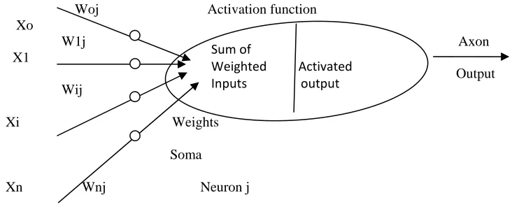
An ANN can be defined as data processing system consisting large number of simple highly interconnected processing elements (PEs or artificial neurons) in architecture analogous to cerebral cortex of brain. An ANN consists of input, hidden and output layers and each layer includes an array of artificial neurons. A typical neural network is fully connected, which means that there is a connection between each of the neurons in any given layer with each of the neuron in next layer. An artificial neuron is a model whose components are analogous to the components of actual neuron (fig1). The array of input parameters is stored in the input layer and each input variable is represented by a neuron. Each of these inputs is modified by a weight (sometimes called synaptic weight) whose function is analogous to that of the synaptic junction in a biological neuron. The neuron (processing element) consists of two parts. The first part simply aggregates the weighted inputs resulting in a quantity I; the second part is essentially a nonlinear filter, usually called the transfer function or activation function. The activation function squashes or limits the values of the output of an artificial neuron to values between two asymptotes. The sigmoid function is the most commonly used activation function. It is a continuous function that varies gradually between two asymptotic values, typically 0 and 1 or-1 and +1.

Woj Activation function Xo

W1j Axon X1

Output Wij

Xi Weights Soma

Xn Wnj Neuron j

Fig 1. Schematic Representation of an Artificial Neuron

ANN Learning

Learning is normally accomplished through an adaptive procedure or algorithm by virtue of which the weights of the connection are incrementally adjusted so as to improve predefined performance measure. The neural network is presented with the data patterns consisting of the input values as well as expected (or output) values. The learning procedure is an iterative process in which the weights are adjusted through an algorithm (e.g. back-propagation algorithm). The objective is to minimize the difference between the predicted output values and expected output values. Initially, because of the random weights assigned to the connections, the difference between the predicted and desired output values can be quite large. Learning, therefore, iteratively adjusts the connection weights to minimize the difference between the predicted and expected output value.

Back- Propagation Training Algorithm

Training of an artificial neural network involves two phases. In the forward pass the input signals propagate from the network input to the output. In the reverse pass, the calculated error signals propagate backward through the network, where these are used to adjust the weights. The calculation of the output is carried out, layer by layer, in the forward direction. The output of one layer is the input to the next layer. In the reverse pass, the weights of the output neuron layer are adjusted first since the target value of each output neuron is available to guide the

Sum of 

Weighted      Activated 

adjustment of the associated weights, using the delta rule. Next, the weights of middle layer (hidden layer) are adjusted. Since the middle layer has no target value, the training is more complicated because the error must be propagated back through the network, including the nonlinear functions, layer by layer. Change of weights in the neuron is given by the equation.

∆w = -η ∂ε2_{/∂w = - ηδø}

(1) Where ∆w = change in weights, η = learning rate, ε = error signal, w = initial weight, ø = output, I = sum of weighted inputs, and δ is defined as 2εq ∂ø/∂I . Thus, the weights in the output and hidden layer neurons can be calculated using equations 2 and 3, respectively.

w(N+1) = w(N) – ηδø (2)

r

w(N+1) = w(N) – ηxΣδq (3) q=1

Where, N = number of iteration, and x = input value.

The above training algorithm is most commonly used and known as the standard back propagation training algorithm. However, one of the major problems of the back propagation algorithm is a local minimum because it employs a form of gradient descent. Thus, it is assumed that the error surface slope is always negative and hence constantly adjusting weights towards minimum. However, error surfaces often involve complex, high dimensional space that is highly convoluted with hills, valleys and folds. Therefore it is very easy for the training process to get trapped in a local minimum.

The problem of the local minima can be avoided by adding a momentum term to weight change (eq.1), to permit larger learning rates. The change of weight is computed as follows.

∆w(N+1) = – η.δ.ø+μ. ∆w(N) (4) where, μ is the momentum coefficient and all other terms are the same as defined earlier. Thus, the new value of weight then becomes equal to the previous value of the weight plus the weight change, which includes the momentum term. Mathematically:

w(N+1) = –w(N)+∆w(N+1) (5) Where, w(N+1) is the weight after N+1 epochs, w(N) is the weight after N epochs and ∆w(N+1) is the change of weight during N to N+1 epochs. By heavily weighting the current weight change based on the previous weight change during the training, the possibility of oscillations are reduced, permitting larger learning rates to be used, thus speeding the training process. This training algorithm is known as back propagation with momentum.

Application of ANN in ETO Estimation

Artificial Neural Network (ANN) approach is utilized to estimate ETo values with limited climatic data (i.e., maximum and minimum temperature only) for MRP command area. Estimated data are further utilized for the prediction of ETo. The ANN models are trained to estimate ETo from weekly and monthly climate data as input and the Penman-Monteith (P-M) estimated ETo as output using the quasi-Newton (Q-N) and backpropagation with variable learning rate (BPVL) algorithms respectively. The model estimates are compared with P-M method estimated ETo. Standard error of estimates (SEE) and model efficiency are used for the performance evaluation of the models. The SEE is an estimate of the mean deviation of the ANN estimate from the P-M method estimated values. It is defined as (Allen, 1986)

)

2

(

)

~

(









n

Y

Y

SEE

(6)

Model Efficiency = 1.0 - ₂ 2

)

(

)

~

(

Y

Y

Y

Y









(7)

where

Y

For the purpose of this study weekly and average monthly climatic data of maximum and minimum temperature, maximum and minimum relative humidity, wind speed, and sunshine hours for the period from January 1986 to December 2005 are used. Weekly and monthly EToare estimated using the P-M method. The P-M estimated ETo values are considered as standard and used for training and testing of ANN models.

Prior to exploring the data to the ANN model for training, the data are normalized. This is done to restrict their range within the interval 0-1. To reach the best generalization, the data set should be split into two parts, namely training set and testing set. The training data set is used to train a neural net by minimizing the error of this data set during training. The testing data set is used for checking the performance of a trained network. Average monthly data set from January 1986 to December 2000 are utilized for training and remaining data from January 2001 to December 2005 used for testing. Weekly data set from January 1986 to December 2001 are utilized for training and remaining data from January 2002 to December 2005 used for testing.

Table 1: Regression and Other Statistics of ETo Values Estimated By ANN, Relative to ETo

Values Estimated By P-M Method

ANN model with configuration

Training algorithm

Time scale

SEE

(mm/d)

Model efficiency

(%)

Coefficient of determination

(r2₎

Slope

(



Intercept

(



ANN model (2-5-1)

quasi-Newton Weekly 0.38 97.63 0.98 0.99 0.071

ANN model

(2-4-1)

BP with variable rate

Monthly 0.58 94.26 0.96 0.96 -0.057

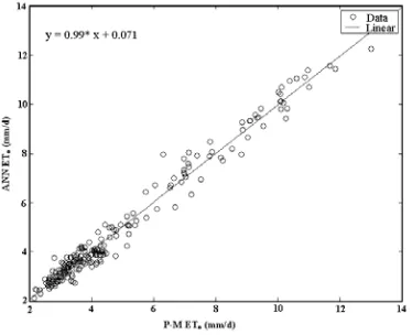
Fig 2: Comparison between ETo values estimated by P-M method and ANN model (2-5-1) trained using

quasi-Newton algorithm for test period from January 2002 to December 2005

Fig 3: Plot between ETo values estimated using P-M method and ANN model (2-5-1) trained using quasi-Newton

algorithm for test period from January 2002 to December 2005

to see which algorithm produces better results for the application under consideration. The ANN model performances are compared with the multiple regression technique.

To obtain the best ANN architecture several possibilities are considered. Determining an appropriate architecture of a neural network for a particular problem is an important issue. The selection of an appropriate input vector that will allow an ANN to successfully map to the desired output vector is not a trivial task (ASCE 2000). Unlike the physically based models, the set of variables that influence the system are not known a priori. However in most of the studies, this problem is addressed through a trial and error procedure. In the present study an attempt has been made to define the input vector based on statistical preprocessing of the data. The autocorrelation and partial autocorrelation function expresses the degree of dependency among the neighbouring observations. Correlation analysis of the time series is employed to see the effects of preceding ETo. Auto and partial autocorrelation statistics and the corresponding 95% confidence bands from Lag 0 to Lag 24 are estimated for the data. The partial autocorrelation function indicates significant correlation up to lag 3 and thereafter, fell within the confidence limits. The analysis suggests that the three antecedent ETo values are adequate in input vector to the ANN models.

For the purpose of the study monthly ETovalues for the period from January 1981 to December 2005 have been used. The data are normalized before being used in to the ANN models. The normalized data is divided into two subsets for the purpose of training and testing. In the present study, 45 data of monthly ETo are used for testing and remaining are used for the training purpose for each network.

Let ETo,trepresents the reference evapotranspiration at time t (month). The following combinations of input data of

ETo are tried: (1) ETo, t-1 , ETo, t-2; (2) ETo, t-1 , ETo, t-2, ETo, t-3; and (3) ETo, t-1 , ETo, t-2 ,ETo, t-3 , ETo, t-4. In all the cases,

output layer has only one neuron, that is, the ETo, t. These three ANN models, based on the input variables are classified as ANN model-1, model-2 and model-3 respectively. For each input, ANN models are trained using three training algorithms namely L-M algorithm, Q-N algorithm and BPVL algorithm. Number of nodes in the hidden layer varied from2 to 13. Using the test input data ETo prediction performance of each network is evaluated. The best ANN architecture for prediction of monthly ETo are selected on the basis of statistical parameters like standard error of estimates (SEE) and model efficiency. The study is extended by applying multiple regression models to the training data following a model calibration using the ETo values used in the testing period of ANN models. Six multiple regression models are tried in the cases in which (i) ETo,t-1 and ETo,t-2 are used as independent variables and

ETo,t is used as dependent variable; (ii) ETo,t-1 , ETo,t-2 and ETo,t-3 are used as independent variables and ETo,t is used as dependent variable; and (iii) ETo,t-1 , ETo,t-2, ETo,t-3 and ETo,t-4 are used as independent variables and ETo,tis used as dependent variable. Total six models are developed based on the procedure outlined in cases (i)-(iii) as above and are presented in Appendix 1. Same training and testing data set of the ANN models are used for the application and calibration of regression relations respectively. Performance of multiple regression models are compared with ANN models. The performance evaluation measures are SEE and model efficiency.

of 3-9-1 trained using quasi-Newton algorithm is found to be the best. This ANN model can be used to predict the

ETovalues which can be utilized to estimate irrigation demands. Conclusions

Monthly crop water requirements of 17 crops sown in command area of MRP system are computed for the period from January 1986 to December 2005. Monthly reference evapotranspiration values are estimated using the preferred Penman-Monteith method. Crop coefficient curves are developed to estimate crop water requirements. Monthly irrigation demands are estimated by considering the rainfall in command area. This study would be useful in deriving optimal operation policies and irrigation scheduling for optimal utilization of stored water. ANN approach is found suitable for the estimation of reference evapotranspiration using limited climatic data (temperature only). ANN approach is also found better than multiple regression technique for prediction of reference evapotranspiration in MRP command area.

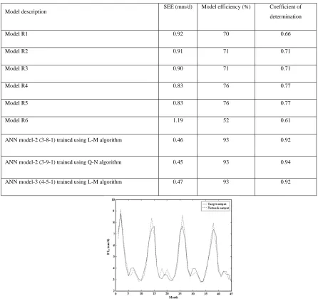
Table 2: Performance Indices and Coefficients of Determination of Regression and Three Selected Artificial Neural Network Models for Testing Data Set

Model description SEE (mm/d) Model efficiency (%) Coefficient of determination

Model R1 0.92 70 0.66

Model R2 0.91 71 0.71

Model R3 0.90 71 0.71

Model R4 0.83 76 0.77

Model R5 0.83 76 0.77

Model R6 1.19 52 0.61

ANN model-2 (3-8-1) trained using L-M algorithm 0.46 93 0.92

ANN model-2 (3-9-1) trained using Q-N algorithm 0.45 93 0.94

ANN model-3 (4-5-1) trained using L-M algorithm 0.47 93 0.92

Fig. 4: Comparison between P-M method estimated ETo and ANN model-2 predicted ETo values for test data with

APPENDIX 5.1: MULTIPLE REGRESSION MODELS FOR FORECASTING ETO OF

MAHANADI RESERVOIR PROJECT COMMAND AREA

 Model R1:

ET



2

.

18



1

.

09

ET



.

59

ET

 Model R2:

ET



2

.

17



1

.

1

ET



.

60

ET



.

003

ET

 Model R3:

ET



2

.

44



1

.

08

ET



.

66

ET



.

16

ET



.

14

ET

 Model R4:

ET



1

.

93

ET

ET

 Model R5:

ET



1

.

85

ET

ET

ET

 Model R6:

ET



.

13

ET

ET

ET

ET

REFERENCES

[1] Allen, R.G. (1986). A Penman for all seasons.” J.Irrig. and Drain. Engg., ASCE, 112 (4):348-368.

[2] Allen, R.G., Jensen, M.E., Wright, J.L. and Burman, R.D.(1989). “Operational estimates of reference evapotranspiration.” Jl. Agron., 81:650-662.

[3] Chiew, F.H.S., Kamaladassa, N.N., Malano, H.M., and McMahon, T.A.(1995). “Penman-Monteith, FAO-24 reference crop evapotranspiration and class-A pan data in Australia.” Agric. Water Mgmt., 28, 9-21.

[4] French M.N., Krajewski W.F. and Cuykendall R.R. (1992). “Rainfall forecasting in space and time using a neural network. “Jl. Hydrol., 137:1-31.

[5] Jain, S.K., Das A. and Srivastava D.K. (1999). “Application of ANN for reservoir inflow prediction and operation”, Jl. Water Resour. Plng. And Mgmt., 125(5):263-271.

[6] Jensen, M.E., Burman, R.D., and Allen R.G. (1990). “Evapotranspiration and irrigation water requirements.” ASCE Manual and Rep. on Engg. Pract. No. 70. ASCE, New York. N.Y.

[7] Minnes, A.W. and Hall M.J. (1996). “Artificial neural networks as rainfall-runoff models” Jl. Hydrologic Sc., 41 (3) : 399-416.

[8] Monteith, J.L. (1965). “The state and movement of water in living organisms.” Proc. Evaporation and Environment, XIXth _{Symp., Soc. For}

Exp. Biol., Swansea, Cambridge University Press, New York, N.Y., 205-234.

[9] Penman, H.L., (1948). “Natural evaporation from open water, bare soil and grass.” Proc. Roy. Soc. London, A193:120-146.