Application of Geostatistical Methods to Estimate Groundwater
Level Fluctuations
Khaled Ahmadaali, Hamed Eskandari Damaneh, Bahareh
Jabalbarezi
International Journal of Advanced Biological and Biomedical Research
Journal DOI:
10.18869/IJABBR
ISSN:
2322-4827
CODEN (USA):
IJABIS
http://ijabbr.com
Copyright © 2018 by authors and the Sami Publishing Corporation (SPC). This work is licensed
under the Creative Commons Attribution International License (CC BY4.0).
11
Available online at
http://ijabbr.com
International Journal of Advanced
Biological and Biomedical Research
6(1) (2018) 11–22
Review Article Open Access
Application of Geostatistical Methods to Estimate Groundwater Level
Fluctuations
Khaled Ahmadaali
1,∗, Hamed Eskandari Damaneh
2, Bahareh Jabalbarezi
31Assistant Professor, Department of Arid and Mountainous Regions Reclamation, Faculty of Natural Resource,
University of Tehran, Iran.
2PhD Student of Desertification, Faculty of Natural Resource, University of Tehran, Iran.
3M.Sc. Expert in Management of Desertification, Faculty of Natural Resource, University of Tehran, Iran.
Abstract
Keeping the water table at a favorable level is quite significant for a sustainable management of groundwater plans. Various management measures need to know the spatial and temporal behavior of groundwater. Therefore, the measurement of groundwater levels are generally carried out at spatially random locations in the field; whereas, most of the groundwater models requires these measurement at a pre-specified grid. Geostatistical techniques could produce an accurate map of groundwater level. Naishaboor plain with 4190 sq km was selected due to presence of over 48 observation wells, mostly with more than 20 years of record. A universal kriging and co-kriging - with level of surface as auxiliary variable - estimator has been used to model groundwater level for three kind of climate condition (wet, normal and dry) and three levels (maximum, average and minimum). The result showed the Gaussian model selected as the best variogram. Furthermore, the RMSE and MRE indicated that kriging method was more accurate than co-kriging in mapping the groundwater level; although, there was not distinct difference.
© 2018 Published by CASRP Publishing Company Ltd. UK. Selection and/or peer-review under responsibility of Center of Advanced Scientific Research and Publications Ltd. UK.
Keywords: Groundwater level, Kriging, SPI, Fluctuation
*Corresponding author: [email protected]
© 2018 The Authors. This is an open access article under the terms of the Creative Commons Attribution-Non Commercial- No Derives License, which permits use and distribution in any medium, provided the original work is properly cited, the use is non-commercial and no modifications or adaptations are made.
12
1. Introduction
Keeping the water table at a favorable level is quite significant for a sustainable management of groundwater plans (Gundogdu and Guney, 2007). Various management measures need to know the spatial and temporal behavior of groundwater (Kumar and Remadevi, 2006). In order to observe water table continuously, groundwater observation wells are used and monthly measurements are normally recorded (Coram et al., 2001). Observed groundwater levels serve as one of the main input data in studies related to groundwater simulation for various purposes as required in water balance studies, estimation of groundwater recharge potential, in the design of drainage structures etc. However, the measurement of groundwater levels are generally carried out at spatially random locations in the field, whereas, most of the groundwater models requires these measurement at a pre-specified grid. Some interpolation method is generally employed to get these values at grid nodes. The accuracy with which this interpolation can be carried out affects the accuracy of the model output.
Kriging is a technique of making optimal, unbiased estimates of regionalized variables at unsampled locations using the structural properties of the semivariogram and the initial set of data values (David, 1977; Gundogdu and Guney, 2007). Basic concepts of the kriging technique and its application to natural phenomenon have been reviewed by the ASCE Task Committee (1990a, b). Kriging has been increasingly used in many branches, such as soil science (Burgess and Webster, 1980; Vieria et al., 1981; Berndtsson and Chen, 1994; White et al., 1997; Bardossy and Lehmann, 1998; Coram et al., 2001); hydrology (Creutin and Obled, 1982; Bastin et al., 1984; Storm et al., 1988; Ahmed and de Marsily, 1989; Germann and Joss, 2001; Araghinejad and Burn, 2005). Kriging of groundwater levels was carried out by (Delhomme, 1978; Volpi and Gambolati, 1978; Chirlin and Dagan, 1980; Aboufirassi and Marino, 1983; Virdee and Kottegoda, 1984; Venue and Pickens, 1992; Kumar, 1996; Kumar and Ahmed, 2003; Kumar and Remadevi, 2006; Gundogdu and Guney, 2007; Ahmadi and Sedghamiz, 2008). Since water level is time varying and is monitored using the same network of observation wells at desired intervals, estimating it for all the time periods following all the steps of geostatistical estimation becomes cumbersome. However, to account for the temporal variation in water level, it is possible to group water level for certain time periods having similar behavior and analyze them geostatistically for spatial variability (Kumar and Ahmed, 2003).
With regarding to the literature review, it is obvious that SPI index have not been used in earlier papers. Consequently, in the present study, the collected monthly water-level data from Naishaboor watershed in the eastern north of Iran have been analyzed geostatistically. Hence, at first, the climate condition of study area was investigated by standardized precipitation index (SPI) and the drought, normal and wet period were determined. Then, in each period, a year was selected in order to assessment the ability of different interpolation methods for diverse climate condition in the Neyshabour watershed.
2. Materials and methods
2.1. Study area and data description
13
Fig. 1. Location of the study area in north eastern of Iran and observation wells in the plain.
At first, the effect of the climate condition on the water table was investigated by SPI index. The Standardized Precipitation Index (SPI) is an index based on the probability of rainfall for any time scale and can assist in assessing the severity of drought. The SPI can be calculated at various time scales which reflect the impact of the drought on the availability of groundwater. This index calculated by the following equation:
Where δi is standard deviation of the ith station data, Xik is precipitation's amount in the ith station and kth
datum and
x
is average of precipitation's amount that this index was calculated by the SPI-SL-6.0 software. Thē
monthly data of groundwater table of 48 observation wells from 1988 to 2004 were used for Geostatistical analyses. Fig. 1 shows the location of observation wells in the plain.2.2. Theory
The main tool in geostatistics is the semivariogram, which expresses the spatial dependence between neighboring observations. The semivariogram quantifies the relationship between the semivariance and the distance between sampling pairs by the following Equation (Isaaks and Srivastava, 1989; Kitanidis, 1997):
У(h) = 1/2n∑n
i=1(Z(xi + h) - Z(xi))2 (2)
Where У(h) is the estimated value of the semivariance for lag(h), n is the number of sample pairs separated by h, Z(xi+h) and Z(xi) are the values of variable Z at xi+h and xi ,respectively, and h is the distance vector between sample points. All pairs of points separated by distance h (lag h) were used to calculate the experimental semivariogram. Spherical, exponential and guassian Models were fitted to the empirical semivariograms. Model selection for semivariograms was done on the bases of determination cofficient (R2), visual fitting and Residual
Sum of Squares (RSS) (Cambardella et al., 1994). Geostatistical software (GS+ Ver.7.0, 2005; Gamma Design software) was used to conduct semivariogram and special structure analysis for variables (groundwater level).
2.3. Interpolation methods 2.3.1. Universal kriging
It is obvious that there was a trend in groundwater flow. For this reason and considering trend in kriging method, the Universal kriging method is selected. Evidently, this method requires knowledge of the structure of
SPI = Xik-
x
̄
(1)14
the trend (which covariates, quadratic terms, interactions?) and of the model-type and parameters of the covariance function or variogram of the residuals. Following model is used for calculating the universal kriging:Z(s) = ∑mj=0βj xj(s) + ε(s) (3)
Where Z(s) is the target environmental variable, s = (s1 s2)′ is a two-dimensional spatial coordinate, xj(s) are
covariates (x0(s) = 1 for all s), βj are regression coefficients, and ε(s) is a normally distributed residual with
zero-mean and constant variance c(0). The residual ε is possibly spatially autocorrelated, as quantified through an autocovariance function or variograms. In what follows it will be convenient to use matrix notation, so that Eq. (3) may be rewritten as:
Z(s) = X'(s)β + ε(s) (4)
Where X and β are column vectors of the m + 1 covariates and m + 1 regression coefficients, respectively. The universal kriging prediction at an unobserved location s0 from n observations z(si) is given by:
Ẑ(s0) = (c0 +X(X'C-1X)-1(X0 - X'C-1c0))' C-1Z (5)
Where X is the n × (m + 1) matrix of covariates at the observation locations, X0 is the vector of covariates at
the prediction location, C is the n × n variance–covariance matrix of the n residuals, c0 is the vector of covariances
between the residuals at the observation and prediction locations, and where Z is the vector of observations z (si).
C and c0 are derived from the variogram of ε.
The universal prediction error variance (universal kriging variance) at s0 is given by (Christensen, 1990):
σ2(s
0) = c(0) - c'0C-1c0 + (X0 - X'C-1c0)' (x'c-1x)-1(x0 - x'c-1c0) (6)
The universal kriging variance incorporates both the prediction error variance of the residual (first two terms on the right-hand side of Eq. (6)), and the estimation error variance of the trend (third term on the right-hand side of Eq. (6)). By minimizing the spatial average (or sum) of the universal kriging variance at points, one automatically obtains the right balance between optimization of the sample pattern in geographic and feature space.
2.3.2. Cokriging
The correlation between different variables is the basis of the cokriging estimator. In this method, by means of an auxiliary variable (level of surface), the principal variable is estimated because the auxiliary variable can be easily measured and there is an existing correlation between auxiliary and principal variables. Supposing Z1 and Z2
are the auxiliary and principal variables, respectively, the following can be written (Isaaks and Srivastava, 1989):
Ẑ(x0) = ∑ni=1λ1iZ1(xi) + ∑mj=1λ2jZ2(xj) (7)
Where Ẑ(χ0) is the estimated principal variable, λ1i and λ2j are the weighting coefficient of auxiliary and
principal variables, respectively. m and n are the numbers of primary and auxiliary samples respectively. For estimating unknown values, the weighting coefficients will be obtained from minimizing the variance of estimation similar to punctual kriging. More details are given in references (Isaaks and Srivastava, 1989; Kitanidis, 1997). As described above, the weights are selected to minimize the estimated error variance (xi). Weights for the primary
variable λ1i are forced to ∑ni=1λ1i = 1, while for secondary variables ∑mj=1λ2j = 0.
2.4. Performance criteria
To evaluate the performance of interpolation methods is used the cross validation method. In this procedure, an observed value is temporarily discarded from the sample data set, and one estimated value at that location is determined using the other sample points. This results in a series of observed and estimated values that can be used to assess the validity of the interpolation method. In this study, estimated and observed values were compared using root mean square error (RMSE), mean absolute error (MAE) and determination coefficient (R2).
RMSE = √1/n∑n
i=1 (Z(xi) - Ẑ(xi))2 (8)
Where n the number of observations is, Z(xi) is the observed value of Z at location (xi), Ẑ(xi) is the estimated
value at the same location and i is the index for the number of data. MRE = 1/n∑n
i=1 [I Z(xi) - Ẑ(xi) I] (9)
15
The smallest MRE is indicative of the most accurate global estimates.3. Results and discussion
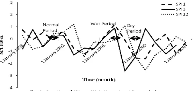
As mentioned earlier, the SPI index was used to determine the wet, normal and dry periods. According to this index, 1991-1992, 1996-1997 and 1999-2000 were categorized as normal, wet and severe drought period respectively. It is obvious that three determined climate condition were critical situation. Therefore, if the kriging estimator was valid for these periods, it would be confirm other climate conditions. The results are shown in Fig. 2.
Fig. 2. Variation of SPI and Wet, Normal and Dry period.
In order to check the anisotropy, the conventional approach is to compare variograms in several directions (Goovaerts, 1997). In this study major angles of 0°, 45°, 90°, and 135° with an angle tolerance of ±22.5 were used for detecting anisotropy. However, there were distinct differences among the structures of the calculated variograms in the four directions so that the angle of 132° was as dominant direction among the other angels because of the best fit with variogram in this direction. Table 1 and 2 shows the parameters of the best fitted prevailing direction variograms obtained based on cross validation.
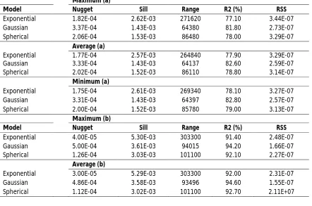
Table 1
Properties of the fitted prevailing direction variograms based on cross validation for kriging estimator and (a) 1991-1992 (Normal period), (b) 1996-1997 (Wet period) and (c) 1999-2000 (severe drought period).
Maximum (a)
Model Nugget Sill Range (m) R2 (%) RSS
Exponential 1.82E-04 2.62E-03 271620 77.10 3.43E-07
Gaussian 3.37E-04 1.43E-03 64380 81.80 2.71E-07
Spherical 2.06E-04 1.53E-03 86480 78.00 3.29E-07
Average (a)
Exponential 1.77E-04 2.57E-03 264840 77.90 3.29E-07
Gaussian 3.33E-04 1.42E-03 64137 82.60 2.59E-07
Spherical 2.02E-04 1.52E-03 86110 78.80 3.14E-07
Minimum (a)
Exponential 1.75E-04 2.61E-03 269340 78.10 3.27E-07
Gaussian 3.31E-04 1.42E-03 64397 82.80 2.57E-07
Spherical 2.00E-04 1.52E-03 85780 79.00 2.31E-07
Maximum (b)
Model Nugget Sill Range R2 (%) RSS
Exponential 4.00E-05 5.30E-03 303300 91.40 2.48E-07
Gaussian 5.00E-04 3.61E-03 94015 94.20 1.66E-07
16
Average (b)
Exponential 4.86E-04 3.58E-03 93496 94.60 2.31E-07
Gaussian 3.00E-05 5.29E-03 303300 92.00 1.55E-07
Spherical 1.12E-04 3.02E-03 101100 92.70 2.11E-07
Minimum (b)
Exponential 4.68E-04 3.40E-03 90066 95.00 2.12E-07
Gaussian 1.00E-05 5.30E-03 303300 92.60 1.44E-07
Spherical 1.03E-04 3.01E-03 101100 93.30 1.93E-07
Maximum (c)
Model Nugget Sill Range R2 (%) RSS
Exponential 1.00E-05 4.73E-03 303300 93.40 3.97E-07
Gaussian 2.20E-04 4.81E-03 111214 96.80 1.15E-07
Spherical 1.00E-06 2.81E-03 101100 94.10 3.07E-07
Average (c)
Exponential 0.00001 4.34E-03 303300 94.80 2.94E-07
Gaussian 1.90E-04 3.59E-03 96873 97.50 7.48E-08
Spherical 1.00E-06 2.58E-03 101100 95.50 2.18E-07
Minimum (c)
Exponential 1.00E-05 4.34E-03 303300 94.80 2.79E-07
Gaussian 2.00E-04 3.55E-03 96527 97.50 7.37E-08
Spherical 1.00E-06 2.58E-03 101100 95.50 2.06E-07
Table 2
Properties of the fitted prevailing direction variograms based on cross validation for co-kriging estimator and (a) 1991-1992 (Normal period), (b) 1996-1997 (Wet period) and (c) 1999-2000 (severe drought period).
Maximum (a)
Model Nugget Sill Range R2 (%) RSS
Exponential 1.82E-04 2.62E-03 271620 77.10 3.44E-07
Gaussian 3.37E-04 1.43E-03 64380 81.80 2.73E-07
Spherical 2.06E-04 1.53E-03 86480 78.00 3.29E-07
Average (a)
Exponential 1.77E-04 2.57E-03 264840 77.90 3.29E-07
Gaussian 3.33E-04 1.43E-03 64137 82.60 2.59E-07
Spherical 2.02E-04 1.52E-03 86110 78.80 3.14E-07
Minimum (a)
Exponential 1.75E-04 2.61E-03 269340 78.10 3.27E-07
Gaussian 3.31E-04 1.43E-03 64397 82.80 2.57E-07
Spherical 2.00E-04 1.52E-03 85780 79.00 3.13E-07
Maximum (b)
Model Nugget Sill Range R2 (%) RSS
Exponential 4.00E-05 5.30E-03 303300 91.40 2.48E-07
Gaussian 5.00E-04 3.61E-03 94015 94.20 1.66E-07
Spherical 1.26E-04 3.03E-03 101100 92.10 2.27E-07
Average (b)
Exponential 3.00E-05 5.29E-03 303300 92.00 2.31E-07
Gaussian 4.86E-04 3.58E-03 93496 94.60 1.55E-07
17
Minimum (b)
Exponential 1.00E-05 5.30E-03 303300 92.60 2.12E-07
Gaussian 4.68E-04 3.41E-03 90066 95.00 1.44E-07
Spherical 1.03E-04 3.00E-03 101100 93.30 1.93E-07
Maximum (c)
Model Nugget Sill Range R2 (%) RSS
Exponential 1.00E-05 4.73E-03 303300 93.40 3.97E-07
Gaussian 2.20E-04 4.81E-03 111214 96.80 1.15E-07
Spherical 1.00E-06 2.81E-03 101100 94.10 3.07E-07
Average (c)
Exponential 1.00E-05 4.34E-03 303300 94.80 2.94E-07
Gaussian 1.90E-04 3.59E-03 96873 97.50 7.49E-08
Spherical 1.00E-06 2.58E-03 101100 95.50 2.18E-07
Minimum (c)
Exponential 1.00E-05 4.34E-03 303300 94.80 2.79E-07
Gaussian 2.00E-04 3.55E-03 96527 97.50 7.37E-08
Spherical 1.00E-06 2.58E-03 101100 95.50 2.06E-07
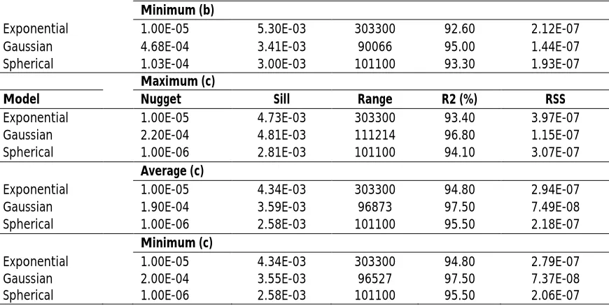
Table 1 is indicated the properties of fitted variograms for Kriging estimator and Table 2 is related to co-kriging estimator. Gaussian model was the dominant type of model that fitted the data because of the low RSS and high R2. Additionally, low nugget effect and consequently low nugget-to-sill ratio generally can be used to classify the spatial dependence (Cambardella et al., 1994). A variable is considered to have strong spatial dependence if the ratio is less than 0.25, and has a moderate spatial dependence if the ratio is between 0.25 and 0.75; otherwise the variable has a weak spatial dependence (Liu et al., 2006). The results in Tables 1 and 2 indicated that in three periods, both estimator and three ground water levels, nugget-to-sill ratio is less than 0.25. As a result, there is a strong spatial dependence among the ground water level data. Obviously, it can be seen from tables 1 to 3 that Gaussian model has the least RSS and the highest R2 for 3 periods and it can be concluded that the Gaussian model in dry period has the least RSS and the highest R2 in compare with the other period. These results are valid for co-kriging method.
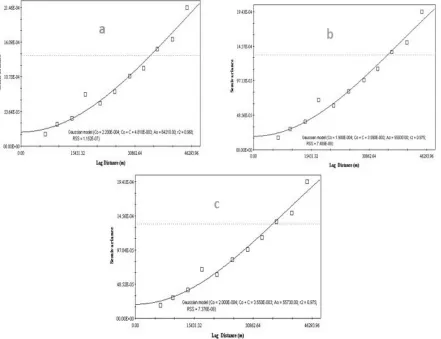
After selecting the Gaussian model, Kriging and co-kriging were applied for estimation of maximum, average and minimum groundwater level across the study area. The performance criteria were applied to the sampled data which were considered for evaluating methods verification. Table 3 summarized the results of applying the performance criteria that mentioned earlier. The plot of the Gaussian semivariogram and the samples are shown in Fig. 3. It is necessary to analyze the spatial variability of the data by semivariance function. Fig. 3 illustrates the semivariance value of primary variables (groundwater table) of the study area.
Table 3
The performance of estimation with kriging and co-kriging methods.
Year Method
Criteria
RMSE MRE
Maximum Average Minimum Maximum Average Minimum
1991-1992 Kriging Co-kriging 19.69 19.96 19.59 19.82 19.58 19.4 0.0124 0.0124 0.0121 0.0122 0.0120 0.0121
1996-1997 Kriging Co-kriging 25.79 25.11 25.26 24.87 24.68 24.59 0.0130 0.0119 0.0129 0.0118 0.0128 0.0118
1999-2000
Kriging 13.41 12.08 12.73 0.0089 0.0079 0.0083
18
Fig. 3. Fitted variograms a) Maximum, b) Average and c) Minimum groundwater level in the study area.
The high value of obtained RMSE can be related to groundwater table which standardized by mean sea level (MSL). If the groundwater table depth was used, the value of RMSE would be very smaller than this result. For this reason, the MRE was used to evaluation the performance of applied methods. The results of table 8 showed that minimum value of RMSE and MRE are related to drought period for two kriging and co-kriging estimator. Also, the normal and wet period were putted in the next rank, respectively as the accuracy. Also, the accuracy of kriging method is higher than co-kriging in estimating groundwater level in three levels (maximum, minimum and average) and for normal and dry period; nevertheless, co-kriging has the better accuracy in wet period for all of the levels.
19
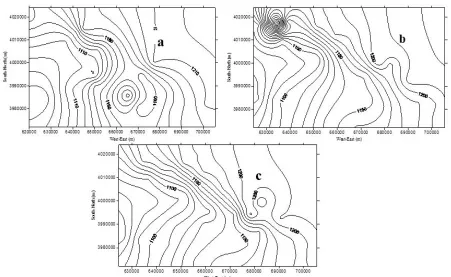
Fig. 4. The kriged map of the groundwater Maximum level a) Normal, b) Wet and c) Dry.
20
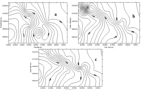
Fig. 6. The kriged map of the groundwater Minimum level a) Normal, b) Wet and c) Dry.
Based on Fig. 4, 5 and 6, it can be observed that the variation of isolevel lines in dry period is very smooth compared with normal and wet periods. The groundwater level in west north parts of the study area varies sharply at short distances in wet period; although, this point not be seen in other climate conditions to such region. This can be related to recharge of plain in this part. Obviously, the density of isolevel lines is greater than normal and dry period. The groundwater isolevel lines in the east northern and west southern parts of the study have relatively less density than other parts. Due to plain topography, the outlet of the watershed is located in the west south part of the region that the kriged map is correspond to this reality. Since kriging is an exact interpolator which honors the real value of the data points during interpolation, and also due to its inherent accuracy in interpolation between known points (Leuangthong et al., 2004), it is believed that applying kriging is helpful in detecting the problematic areas, and aids the managers in management of water resources (Ahmadi and Sedghamiz, 2007).
4. Conclusion
21
References
Aboufirassi, M., Marino, M.A., 1983. Kriging of water levels in the souss aquifer Morocco. Math. Geol., 15, 537-551. Ahmadi, S.H., Sedghamiz, A., 2008. Application and evaluation of kriging and cokriging methods on groundwater
depth mapping. Environ. Monit. Assess., 138, 357-368.
Ahmed, S., de Marsily, G., 1989. Cokriged estimates of transmissivities using jointly water level data, In: Armstrong, M., (ed.), Geostatistic, Kluwer Academic Pub., 2, 615-628.
Araghinejad, S., Burn, D.H., 2005. Probabilistic forecasting of hydrological events using geostatistical analysis. Hydrol. Sci. J., 50, 837-856.
ASCE Task Committee, 1990a. Review of geostatistics in geohydrology, I: Basic concepts. J. Hydraul. Eng. (ASCE), 116, 612-632.
ASCE Task Committee, 1990b. Review of geostatistics in geohydrology, II: Applications. J. Hydraul. Eng. (ASCE), 116, 633-658.
Bardossy, A., Lehmann, W., 1998. Spatial distribution of soil moisture in a small catchment. Part I: Geostatistical analysis. J. Hydrol., 206, 1-15.
Bastin, G., Lorent, B., Duque, C., Gevers, M., 1984. Optimal estimation of the average rainfall and optimal selection of raingage locations. Water Resour. Res., 20(4), 463-470.
Berndtsson, R., Chen, H., 1994. Variability of soil water content along a transect in a desert area. J. Arid Environ., 27, 127-139.
Burgess, T.M., Webster, R., 1980. Optimal interpolation and isarithmic mapping of soil properties, I: The semivariogram and punctual kriging. J. Soil Sci., 31, 315-331.
Cambardella, C.A., Moorman, T.B., Novak, J.M., Parkin, T.B., Karlen, D.L., Turco, R.F., 1994. Field scale variability of soil properties in Central Iowa soils. Soil Sci. Soc. Am. J., 58, 1501-1511.
Chirlin, G.R., Dagan, G., 1980. Theoretical head variogram for steady flow in statistically homogeneous aquifers. Water Resour. Res., 16(6), 1001-1015.
Christensen, R., 1990. Linear models for multivariate, time, and spatial data. Springer, New York.
Coram, J., Dyson, P., Evans, R., 2001. An evaluation framework for dryland salinity, report prepared for the National Land & Water Resources Audit (NLWRA), sponsored by the Bureau of Rural Sciences, National Heritage Trust, NLWRA and National Dryland Salinity Program, Australia.
Creutin, J.D., Obled, C., 1982. Objective analysis and mapping techniques for rainfall fields: An objective comparison. Water Resour. Res., 18, 413-431.
David, M., 1977. Geostatistical ore reserve estimation. Developments in Geomathematics 2. Elsevier (Amsterdam), 364p.
Delhomme, J.P., 1978. Kriging in the hydroscience. Adv. Water Resour., 1, 251-266.
Gamma Design Software, 2005. GS+ Geostatistics for the environmental science version 7.0. Gamma Design software L.L.C., Plainwell, Michigan, USA.
Germann, U., Joss, J., 2001. Variograms of radar reflectivity to describe the spatial continuity of apline precipitation. J. Appl. Meteorol., 40, 1042-1059.
Goovaerts, P., 1997. Geostatistics for natural resources evaluation. New York: Oxford University Press.
Gundogdu, K.S., Guney, I., 2007. Spatial analysis of groundwater levels using universal kriging. J. Earth Syst. Sci., 116(1), 49-55.
Hoseini, A., Farajzadeh, M., Velayati, S., 2005. The water cresis analyses from the approach of environmental in the Neishaboor plain. Research committee of water organization of Khorasan Razavi province.
Isaaks, E., Srivastava, R.M., 1989. An introduction to applied geostatistics. New York: Oxford University Press. Kitanidis, P.K., 1997. Introduction to geostatistics: Application to hydrogeology. Cambridge, UK: Cambridge
University Press.
Kumar, D., Ahmed, S., 2003. Seasonal behaviour of spatial variability of groundwater level in a granitic aquifer in monsoon climate. Curr. Sci., 84, 188-196.
Kumar, V., 1996. Space time modeling of ground water with assistance of remote sensing. Ph.D. Indian Institute of Technology, New Delhi, India.
Kumar, V., Remadevi, 2006. Kriging of groundwater levels - A case study. J. Spatial Hydrol., 6(1), 81-90.
22
Storm, B., Jenson, K.H., Refsgaard, R.C., 1988. Estimation of catchment rainfall uncertainty and its influence onrunoff prediction. Nord. Hydrol., 19, 79-88.
Velayati, S., Tavassoli, S., 1991. The resources and the problems of Khorasan's water. Astane Ghodse Razavi, Mashhad, Iran.
Vieira, S.R., Nielsen, D.R., Biggar, J.W., 1981. Spatial variability of field measured infiltration rate. Soil Sci. Soc. Am. J., 45, 1040-1048.
Virdee, T.S., Kottegoda, N.T., 1984. A brief review of kriging and its application to optimal interpolation and observation well selection. Hydrol. Sci. J., 29, 367-387.
Volpi, G., Gambolati, G., 1978. On the use of main trend for the kriging technique in hydrology. Adv. Water Resour., 1, 345-349.
White, J.G., Welch, R.M., Norvell, W.A., 1997. Soil zinc map of the USA using geostatistics and geographic information systems. Soil Sci. Soc. Am. J., 61(1), 185-194.