Characteristic Time of Diffusive Mixing in Cube with Reflecting Edges

http://www.sciencepublishinggroup.com/j/ajmp doi: 10.11648/j.ajmp.20170605.11

ISSN: 2326-8867 (Print); ISSN: 2326-8891 (Online)

Characteristic Time of Diffusive Mixing in Cube with

Reflecting Edges

Gurami Tsitsiashvili

Institute for Applied Mathematics FEB RAS, Vladivostok, Russia

Email address:

[email protected]

To cite this article:

Gurami Tsitsiashvili. Characteristic Time of Diffusive Mixing in Cube with Reflecting Edges. American Journal of Modern Physics. Vol. 6, No. 5, 2017, pp. 81-87. doi: 10.11648/j.ajmp.20170605.11

Received: June 30, 2017; Accepted: July 11, 2017; Published: July 31, 2017

Abstract:

V. V. Uchaikin suggested a mathematical model of an anomalous diffusion in a space. These model origins in an investigation of processes in complex systems with variable structure: glasses, liquid crystals, biopolymers, proteins and a turbulence in a plasma. Here a coordinate of diffusing particle has stable distribution and so its density satisfies diffusion equation with partial derivatives. In this paper, the anomalous diffusion with periodic initial conditions on an interval with reflecting edges, important for example in technical mechanics, is considered and analyzed.

Keywords:

Anomalous Diffusion, Reflecting Edges, Partial Derivatives

1. Introduction

In [1] a mathematical model of an anomalous diffusion in a space was suggested. These model origins in an investigation of processes in complex systems with variable structure: glasses, liquid crystals, biopolymers, proteins and a turbulence in a plasma [2].

In this model a coordinate of diffusing particle has stable distribution (not normal one). As a result a density of its distribution satisfies an analogy of diffusion equation in which second derivative by coordinate is replaced by partial derivative.

In this paper the anomalous diffusion with periodical initial conditions on an interval with reflecting edges is considered. Such problem is important for example in technical mechanics for an analysis of fuel mixing in straight flow engine [3] too.

Suppose that y t( ), t≥0, is homogeneous random process with independent increments and an initial condition

(0) = 0.

y A random variable y t( )−y( ),τ t>τ ≥0, has symmetric stable distribution on the straight line (−∞ ∞, ) with a parameter a, 0 <a≤2, and a characteristic function

exp( [ ( ) ( )]) = exp( ( ) | | ).a

M i u y t −y

τ

− −t

τ

u (1)

The distribution density pt = p ut( ) of the process y t( ) in a moment t> 0 is generalized solution of the following

differential equation with fractional derivatives [1].

( ) = ( ) ( ).

a t

a p y y t

t y

δ δ

 _{∂ ∂} 

−

 

_{∂ ∂} 

 

Here ∂ap y_t( ) /∂ya is a -fractional derivative of the function p y_t( ), 0 <a≤2, δ( ),y δ( )t are delta-functions by variables y t, accordingly.

It is impossible to use the method of Fourier series to analyze anomalous diffusion on segment with reflecting edges. To get over this difficulty in this paper an analogy with the wave equation for finite string with fixed edges is used. Some approaches to generalize one-dimensional results are considered. Main analytical results of this paper have been obtained in [4]. But in this paper these results are supplemented by physical interpretation and consideration of diffusion in multidimensional cube with reflecting boundaries.

2. Diffusion on Segment with Reflecting

Edges

Assume that y t( ), t≥0, is uniform random process with

independent increments; y(0) = 0. Difference

( ) ( ), > 0,

distribution with parameter a, 0 <a≤2, and the characteristic function (1). The process y t( ), t≥0, describes in [1] anomalous diffusion on infinite straight line.

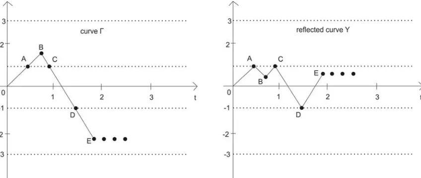
2.1. Geometric Representation

Each realization of random process y t( ), t≥0, may be considered as a curve Γ on the plane ( , ).y t Suppose that the curve Γ is reflected from the lines y= 1,y= 1.− For this aim represent the plane ( , )y t as a transparent and infinitely thin sheet of paper with the curve Γ. Bend this sheet of the

paper along the lines y= 1,± y= 3,± into transparent strip

1 y 1

− ≤ ≤ with fragments of the initial curve Γ. The curve

Γ converted into the curve

γ

described by the process

( ), 0.

Y t t≥ Similar [1] the random process Y t( ), t≥0 may be interpreted as a model of the anomalous diffusion on the interval [ 1, 1]− with reflecting edges. It is clear that if the curve Γ coincides with some straight line then the curve

γ

constructing in an accordance with the law of geometrical optics: falling angle equals to reflecting angle.

Figure 1. Construction of reflected curve

γ

.

2.2. Analytical Representation

Additionally to geometric representation of the process,

( ), 0,

Y t t≥ we give its analytic representation by means of the functions f R: → −[ 2, 2),g: [ 2, 2)− → −[ 1, 1].

, 1 1,

( ) = ( 2) / 4 2, ( ) = 2 , 1 < < 2,

2 , 2 < 1

u u

f u u mod g u u u

u u

− ≤ ≤

 

+ −  −

_{− − − ≤ −}



Figure 2. Graphics of functions f g, .

Then Y t( ) = g f y t( ( ( ))).

2.3. Reflection Formula

Assume that p_t = p u_t( ),P_t =P u_t( ),π_t =π_t( )u are densities of random variables y t( ), f y t( ( )), ( )Y t

distributions. Using the function f graphics (see also Figure 2) obtain:

=

( ) = ( 4 ), [ 2, 2), ( ) = 0, [ 2, 2).

t t t

k

P u p u k u P u u

∞

−∞

− ∈ − ∈ −/

∑

(2)

=

( ) = ( 2 ), [ 1, 1], ( ) = 0, [ 1, 1].

t t t

k

u p u k u u u

π ∞ π

−∞

− ∈ − ∈ −/

∑

(3)

Remark that Formula (3) which gives distribution density of diffusion reflected process is analogous to reflection method formula which gives solution of wave equation for finite string with fixed edges [5, chapter III, §13, points 5, 6].

2.4. Rate Convergence to Uniform Distribution

Define auxiliary function

=

( ) = ( 4 ), < <

t _k t

P u ∞ p u k u

−∞ − − ∞ ∞

∑

,

it coincides with P u_t( ) for u∈ −[ 2, 2), has period 4 and is even. Denote q u v_t( , ) =P v ut( − ), − ≤2 u v, < 2,

= inf{ ( , ), 2 , < 2},

t t

Q q u v − ≤u v then from Formula (2) we have

0 <Qt ≤1 / 4, t> 0. (4) Put

1 / 4, [ 2, 2), 1 / 2, [ 1, 1],

( ) = ( ) =

0, [ 2, 2), 0, [ 1, 1].

u u

P u u

u π u

∈ − ∈ −

 

 

∈ −/ ∈ −/

 

For functions ( ),φ u ψ( )u defined on, (−∞ ∞, ), introduce a norm

1

( )u ( )u _C= sup{| ( )u ( ) |,u <u< },

φ

−

ψ

φ

−

ψ

− ∞ ∞

believing [ ]z integer part of real number .z

Lemma 1. For arbitrary t≥1 the following inequality is true:

1 1

[ ] 1 1 1

||

π

_t( )u −

π

( ) ||u _C≤2(1 4− Q)t− || ( )P u −P u( ) ||_C . (5)

Remark that Lemma 1 is true for any even distribution densityp u_t( ), which satisfies Formula (4).

2.5. Self-similarity of Anomalous Diffusion

Next consideration closely connecting with a concept of a self-similar random process (see for example [6]) has a large application in modern physics [7-10].

Assume that r> 0, consider Markov process ( ) = ( ( ( ) / )), 0.

r

Y t rg f y t r t≥ The process Y t tr( ), ≥0, is obtained from random process y t( ),t≥0, by reflection from edges of the segment [−r r, ]. Denote

π

t r, =

π

t r, ( )u

distribution density of random variable Y t_r( ). It is obvious that

π

_{t, 1}=

π

_t.

Lemma 2. For [t r−a] 1≥ the following inequality is true:

1 1

[ ] 1

1 1

,

2(1 4 ) || ( ) ( ) ||

|| ( ) ( / ) / || .

a t r

C

t r C

Q P u P u

u u r r

r

π −π ≤ − − − − (6)

Formula (6) is based on self-similarity property of the

process Y t( ) and may be interpreted as an increasing (or a

decreasing dependently on r) in ra times of characteristic mixing time of anomalous diffusion on segment [−r r, ] in a comparison with diffusion on segment [ 1,1].− For r< 1 anomalous diffusion “works” slower and for r> 1 works faster than normal diffusion.

2.6. Periodical Initial Conditions

Diffusion process with periodical initial conditions origins for example in fuel mixing at straight flow engine [3, chapter 7, § 7.1]. For its modelling, take natural n and define Markov process

( ) = ( ( ( ) (0))), 0

n n

Z t g f y t +Z t≥

.

Here random process y t( ) and random variable Z_n(0) are independent and Z_n(0) has continuously differentiable distribution density r u_n( ), which satisfies conditions: of a periodicity

(

)

( ) = 2 / , 1 1 2 / ,

n n

r u r u+ n − ≤ ≤ −u n

of a symmetry

(

)

( 1 1/ ) = 1 1/ , 0 1/ ,

n n

r − + n v− r − + n v+ ≤ ≤v n

and boundary conditions

( )

= 0 = 1.

n

dr v

for v

dv ±

Then random process Z t_n( ), t≥0, may be considered as anomalous diffusion on the segment [ 1, 1]− but with periodical initial conditions, defined by distribution density

( ).

n

r u Denote Πt n, =Πt n, ( )u distribution densities of r.

v.‘s Z t_n( ), t> 0.

Lemma 3. The following formula is true

1

, ,1/ =0

1 2 1

( ) = 1 .

n t n t n

k

k

u u

n

π

n

− _{ + }

Π  + − 

 

∑

(7)

The equality (7) means that the diffusion (normal or anomalous) on the segment [ 1, 1]− with periodical initial conditions and reflecting edges leads to the same result as a diffusion on isolated (by reflecting edges) sub segments

2 1 1 2 3 1

1 k , 1 k , k= 0, ,n 1,

n n n n

+ +

 

− + − − + + −

 

  …

of the segment [ 1, 1].−

Remark that the equality (7) is true for each self-similar random process y t( ) with independent and symmetrically distributed increments.

1 1 [ ] 1

, 1 1

||Π_{t n}( )u −π( ) ||u _C≤2(1 4− Q)t na− ||P u( )−P u( ) ||_C .(8)

Formula (8) is interpreting as a decreasing in na times of characteristic mixing time of anomalous diffusion on the segment [ 1,1]− with periodical initial conditions.

2.7. Numerical Experiment

Obtained analytical results comparing here with results of numerical experiment and a closeness of densities π πt, for different t are estimated. For this aim, independent random variables with distributions of Y t( ), coinciding with a

distribution of random variable g f t( (1/ay(1))) are imitated by Monte-Carlo method. Random variable y(1) is imitated approximately by normed sum

1 1/

ˆ(1) = N

a

v v

y

N

+ +…

of independent and equally distributed random variables

1, , N,

v … v

1 1

( > ) = a / 2, ( < ) = a / 2, > 1.

P v t t− P v −t t− t

By M independent realizations of g f t( (1/ayˆ(1))), coinciding with Y t( ) (by distribution), we construct

frequencies S t_j( ), j= 0,…,9, of these realizations belonging to sub segments

2 2( 1) 2

1 , 1 , = 0, ,8, 1 , 1 , = 9.

10 10 10

j j j

j j

+

   

− + − +  −

  

  …  

Analogously with statistics of Chi-square we calculated

2 9

=0

1

( ) = 10 ( ) ,

10

j j

S t M S t − 

 

∑

characterizing a deviation of random variable Y t( ) distribution from uniform distribution for different t.

Table 1. Results of numerical experiment.

t S(t) for a=1.9 S(t) for a=1.95 S(t) for a=1.99

0.01 9169.31 7867.49 6584.26

t S(t) for a=1.9 S(t) for a=1.95 S(t) for a=1.99

0.02 4055.39 3053.09 2537.75 0.03 2200.99 1298.15 1017.17 0.04 1061.13 609.86 347.35 0.05 488.14 289.15 185.43 0.06 220.69 177.32 122.32 0.07 135.03 52.97 39.26 0.08 102.79 39.37 13.26 0.09 54.89 14.55 12.78

Table 1 shows qualitative coincidence of numerical results with estimates of Formula (8). If a→2 then rate convergence of Y t( ) to uniform distribution density increases. However, it is necessary to remark that an increasing of t demands an increasing of N that complicates numerical experiment.

3. Multidimensional Diffusion on Square

with Reflecting Boundaries and

Periodical Initial Conditions

In this section, we consider as normal so anomalous diffusion on k - dimensional square with reflecting boundaries. Normal diffusion is analyzed by the method of Fourier series but for anomalous diffusion it is more convenient to use the reflection formula.

3.1. Multidimensional Normal Diffusion

Consider a model of k- dimensional normal diffusion in the cube [ 1,1] ,− k k= 2,3, with reflecting boundaries. Assume that Πt n, ( ,y1…,yk) is a density of a distribution of

diffusing particle coordinate at a moment t in a point

1

( ,y …,y_k) [ 1,1] :∈ − k

2

, 1 2

=1

( , , ) = 0,

k

t n k r

r

y y

t y

_{∂ ∂} 

− Π

 

_{∂ ∂} 



∑



…

, ( 1, , 1, , 1, , 1) = 0, 1 1, = 1, , ,

t n r r

r

y y r k

y

∂ Π ± ± ± ± − ≤ ≤

∂ … … …

1

0, 1 1

, , =1 =1

1

( , , ) = ( , , ) cos > 0.

2

k

k

n k _k k r r

j j r

y y a j j πn j y

∞

Π +

∑

∏

…

… …

Then we have the following equality

1

2 2 2

, 1 1

, , =1 =1 =1

1

( , , ) = ( , , ) cos exp .

2

k

k k

t n k k k r r r

j j r r

y y a j j πn j y π n t j

∞  

Π + − 

 

 

∑

_∏

∑

…

… …

For a function, l y( ,₁…,y_k), ( ,y₁ …,y_k) [ 1,1] ,∈ − k define a norm

2

1 1 2

1 1 1

1 1

|| ( , , ) || = ( , , )

k

k _L k k

l y y dy dy l y y

− −

∫

∫

… … … ,

2 1

2 2 2 2

, 1 1

, , =1 =1

1

( , , ) = ( , , ) exp 2 .

2 _k

k

k

t n k k k r

L j j r

y y a j j

π

n t j

∞ _{ }

Π − − 

 

 

∑

∑

…

… …

If a i( ,1…, )ik ≠0 and

2 2

1 1

=1 =1

< , 1 , , < , ( , , ) 0,

k k

r r k k

r r

i j ≤ j j ∞ a j j ≠

∑ ∑

… …

then

2 2

2 2 2

, 1 0, 1 1

=1

1 1

( , , ) exp ( , , ) .

2 2

k k

k

t n k _k r k _k

L r L

y y π n t i y y

 

Π − ≤ −  Π −

 



∑



… …

Consequently, it is possible to choose n- periodical initial condition so that in the cube [ 1,1]− k characteristic mixing

time decreases in 2 2

=1

k r r

n

∑

i times. In such a way, it is

possible to decrease characteristic time dependently on Fourier coefficients of initial condition Π_0,1( ,y₁…,y_k).

3.2. Multidimensional Anomalous Diffusion

Consider k - dimensional diffusion

1

( ( ),Y t …,Y t_k( )), k= 2, 3, with independent components distributed as Y t( ) (defined by the parametera) and with n-

periodical initial conditions ₁( )

=1 ( ).

k _j j j P u

∏

Then its

distribution density may be represented as

( )

, 1 ,

=1

( , , ) = ( ).

k j t n k t n j

j

u u u

Π …

∏

Π

Denote limit uniform distribution

( )

1 ₌₁

( , , _k) = k j ( _j)

j

u u u

π …

∏

π with

( )

( ) = ( ).

j

u u

π

π

From

Theorem 1 we have the inequality

1 1

( )

( ) ( ) [ ] 1 ( )

, ( ) ( ) 2(1 4 1) || 1 ( ) ( ) || = , , 1.

a j

j j j t n j a

t n j j j C t n

C

u π u Q − P u P u t n

Π − ≤ − − ∆ ≥ (9)

For functions Φ( ,u₁…,u_k),Ψ( ,u₁…,u_k)defined on the cube, [0,1]

k _{introduce a norm}

1 1 1 1 1

( , , ) ( , , ) = sup{| ( , , ) ( , , ) |, < , , < }.

k

k k C k k k

u u u u u u u u u u

Φ … − Ψ … Φ … − Ψ … − ∞ … ∞

Then it is easy to prove the following statement. Theorem 2. Assume that t n1/a ≥1 then for k= 2

2

, 1 2 1 2 , , ||Π_{t n}( ,u u )−

π

( ,u u ) ||_C ≤ ∆_{t n}(1+ ∆_{t n}).

And for k= 3

(

)

3

2

, 1 2 3 1 2 3 , , ,

||Πt n( ,u u u, )−π( ,u u u, ) ||C ≤ ∆t n 3 / 4 3 / 2+ ∆ + ∆t n t n .

4. Example: Mixing of Impurity in

Straight flow Engine

In an analysis of impurity blowing in an airflow, we simplify its picture to divide the most important parameters influencing on a mixing time. Therefore, we assume that a process of an impurity mixing consists of two stages. In first stage, an impurity consists of separate particles, which move as Stokes particles and do not diffuse before their merger with the airflow. In second period impurity, particles diffuse in cross direction to the airflow.

4.1. Merger of Injected Stokes Particle with Airflow

Consider first stage when impurity particles move independently each other’s. To simplify considered problem we believe that the airflow is uniform and different ripples do not influence on particles behavior, physical properties of matters are constant.

Assume that Stokes particle with a mass m is injected with a velocity v in direction x perpendicularly air flow moving with a velocity V in plane channel which has a width l in direction y (see Figure 3). Define particle coordinates ( , )x y to moment when impurity particle mergers with the airflow. Related motion equations have the following form

= _x, = _y, (0) = 0, (0) = 0.

dx dy

v v x y

dt dt

= , y = ( ), (0) = , (0) = 0.

x

x y x y

mdv mdv

kv k v V v v v

Here v_x,v_y are velocities of Stokes particle, k is friction coefficient. The system of motion equations has following solution

( ) = (1 exp( / )), ( ) = ( (1 exp( / ))),

x t vT − −t T y t V t T− − −t T

( ) = exp( / ), ( ) = (1 exp( / )), = / .

x y

v t v −t T v t V − −t T T m k

So x t( )→vT t, → ∞. Consequently characteristic time of Stokes particle merging with the airflow (characteristic time of velocity relaxation of impurity) is T and a depth of Stokes particle penetration is vT.

Figure 3. Injection of impurity into airflow.

4.2. Cross Diffusion of Injected Particles in Airflow

Consider now second stage of Stokes particle mixing with the airflow. Assume that in a moment (of intermediary asymptotic) t₀ =T Stokes particles have a concentration

0( )

c x in a segment [0, ]l .

For t0 >T we solve diffusion equation for impurity

concentration ( , ),c x t x∈[0,1], T< <t ∞:

2

2

( , ) = ( , )

c x t D c x t

t x

∂ ∂

∂ ∂

with diffusion coefficient D , the following boundary (neprocitana) conditions

=0 =

( , ) |_x = ( , ) |_{x l}= 0, 0,

c x t c x t t

x x

∂ ∂ _≥

∂ ∂

and initial condition

0

( , 0) = ( ), 0

c x c x ≤ ≤x l.

The initial condition defining by results of first stage is

n-periodic function:

0 0 0

1

= ( ), 0 1 , ( ) = ( ), 0 ,

l l

c x c x x l c x q nx x

n n n

   

+ ≤ ≤ − ≤ ≤

   

   

where

4 2 0

=1 =1

( ) = _kcos 2 , _k < .

k k

x

q x q a k k a

l

π

∞ ∞

+

∑

∑

∞

This problem has the following solution by the Fourier series method:

2

0 =1

2 2

( , ) = _kcos exp .

k

knx nk

c x t q a Dt

l l

π π

∞  _{ } 

 

+ _−  _

 

 

∑

Consequently, characteristic mixing time T_n satisfies the relations

1 1 2

1

, = .

2

n

T l

T T

k D

n π

 

≈  

 

To obtain initial conditions as n-periodic function it is convenient to make n holes for impurity injection and to choose injection velocities v in accordance with the relation that a depth of Stokes particle penetration is vT.

Figure 4. Cross diffusion of impurity.

5. Conclusion

It is interesting to mark that suggested scheme of mixing time calculation may be used not only for anomalous diffusion but also for diffusion described by fractional Brownian motion. In this case, it is impossible to use the Fourier series method. However, a representation described in Figure 1 allows getting over this difficulty. Diffusion models with fractional Brownian motion are considered as in physical [7] so in informatics applications [12]. Some last results for multivariate fractional Levi motion (but without reflecting from segment ends) are obtained in [13].

References

[1] Uchaikin V. V. Multidimensional symmetric anomalous diffusion. Chemical Physics. Vol. 284, 2002, pp. 507-520. [2] Skvortsova N. N, Batanov G. M, Petrov A. E, Pshenichnikov A.

A, Sarksyan K. A, Kharchev N. K. Non-Brownian Particle Motion in Structural Plasma Turbulence. Proceedings of the XXIII Seminar on Stability for Stochastic Models. Pamplona, Spain, 2003, p. 88.

[4] Tsitsiashvili G. Sh. Anomalous Diffusion on Finite Interval. Journal of Mathematical Sciences. Vol. 191, issue 4, 2013, pp. 582-587.

[5] Vladimirov V. S. Equations of mathematical physics. Moscow: Nauka, 1967. (In Russian).

[6] Embrechts P, Maejima M. An introduction to the theory of self-similar stochastic processes. International journal of modern physics B. Vol. 12-13, 2000, pp. 1399-1420.

[7] Chen S. et al. Self-similar Random Process and Chaotic Behavior. In Serrated Flow of High Entropy Alloys. Sci. Rep. Vol. 6, 2016. Doi 10.1038/srep 29798.

[8] Caroll R. et al. Experiments and Model for Serration Statistics in Low-Entropy, Medium Entropy Alloys. Sci. Rep. Vol. 5, 2015. Doi 10.1038/srep 16997.

[9] Zhang Z. J. et al. Nanoscale origins of the damage tolerance of the high-entropy alloy CrMnFeCoNi. Nat Commun. Vol. 6, 2015. PMC free article [PubMed].

[10] Youssef K. M. et al. A novel low density, high-hardness, high entropy alloy with close packed single-phase nanocrystalline structures. Mater Res Lett. Vol. 3 (2), 2015.

[11] Feller W. Introduction to probability theory and its applications. Moscow: Mir, T. 2, 1984. (In Russian).

[12] Mikosch T. et al. Is network traffic approximated by stable Levy motion or fractional Brownian motion? Annals of Applied Probability. Vol. 12, no. 1, 2002, pp. 23-68.