M E T H O D O L O G Y
Open Access
Sparse generalized linear model with
L
0
approximation for feature selection and
prediction with big omics data
Zhenqiu Liu
1*, Fengzhu Sun
2and Dermot P. McGovern
3*Correspondence: [email protected] 1Samuel Oschin Comprehensive Cancer Institute, Cedars-Sinai Medical Center, Los Angeles 90048, CA, USA
Full list of author information is available at the end of the article
Abstract
Background: Feature selection and prediction are the most important tasks for big
data mining. The common strategies for feature selection in big data mining areL1,
SCAD and MC+. However, none of the existing algorithms optimizesL0, which
penalizes the number of nonzero features directly.
Results: In this paper, we develop a novel sparse generalized linear model (GLM) with
L0approximation for feature selection and prediction with big omics data. The proposed
approach approximate theL0optimization directly. Even though the originalL0problem
is non-convex, the problem is approximated by sequential convex optimizations with the proposed algorithm. The proposed method is easy to implement with only several
lines of code. Novel adaptive ridge algorithms (L0ADRIDGE) forL0penalized GLM with
ultra high dimensional big data are developed. The proposed approach outperforms the other cutting edge regularization methods including SCAD and MC+ in simulations. When it is applied to integrated analysis of mRNA, microRNA, and methylation data from TCGA ovarian cancer, multilevel gene signatures associated with suboptimal debulking are identified simultaneously. The biological significance and potential clinical importance of those genes are further explored.
Conclusions: The developed SoftwareL0ADRIDGE in MATLAB is available at https://
github.com/liuzqx/L0adridge.
Keywords: Sparse modeling,L0penalty, Big data mining, Multi-omics data, GLM,
Classification, Suboptimal debulking
Background
Integrating multilevel molecular and clinical data to design preventive, diagnostic, and therapeutic solutions that are individually tailored to each patient’s requirements is the ultimate goal of precision medicine. However, the huge number of features makes it nei-ther practical nor feasible to predict clinical outcomes with all omics features directly. Thus, selecting a small subset of informative features (biomarkers) to conduct association studies and clinical predictions has become an important step toward effective big data mining. Statistical tests or univariate correlation analysis for feature selection ignore the interacting relationship among genes. To evaluate the predictive power of the features, one appealing approach for feature selection isL0regularized sparse modeling, which
penalizes the number of nonzero features directly.L0is known as the most essential spar-sity measure and has nice theoretical properties. However, it is computational impossible to perform an exhaustive search when analyzing omics data sets with millions of features. L0penalized optimization is known to be NP-hard in general (Lin et al. 2010).
One common strategy for feature selection is to replace the non-convexL0with theL1 norm.L1is a convex relaxation and loose approximation ofL0. AlthoughL1penalized sparse models [1] can be solved efficiently, the estimators withL1are penalized too much and asymptotically biased. In addition,L1inclines to select more spurious features than necessary, and may not always choose the true model consistently [2]. Theoretically,L1 never outperformsL0by a constant [3]. Depending on the location of true optimum,L1 may perform much worse thanL0 [4, 5]. As a result, the convex relaxation techniques have been shown to be suboptimal in many cases [6]. More recent approaches aimed to reduce bias and overcome discontinuity include the non-convex SCAD [7] and MC+ [8]. However, none of the existing algorithms directly approximate theL0optimization prob-lem. Either SCAD or MC+ has been rarely used for feature selection in big data analytics because of their computational intensity with multiple tuning parameters. On the other hand, recent research works including ours show that sparse regression models withL0 penalty (local solution) outperformsL1(global solution) by a substantial margin [5, 9–11]. Debulking cytoreductive surgery is a standard treatment for ovarian cancer. The goal of debulking is to remove as much visible cancer as possible. However, if tumor nodules have invaded vital organs, surgeons may not be able to remove them without compro-mising the patient’s life. Leaving tumor nodules larger than 1 cm is defined as suboptimal debulking (cytoreduction). It has been shown that suboptimal debulking is associated with reduced chemosensitivity and poor survival in ovarian cancer. Biomarkers derived from multi-omics data may help physicians decide which patients should undergo surgery and which should be treated with chemotherapy first [12–14]. Identifying biomarkers from multi-omics data has been an exciting but challenging task. Sparse modeling is one of the important approaches for simultaneous phenotype prediction and biomarker iden-tification. In this paper, we propose aL0penalized generalized linear regression (GLM) for feature selection and prediction. Adaptive ridge algorithm (L0ADRIDGE) is developed to approximateL0penalized GLM with sequential convex optimization and is efficient in handling ultra high-dimensional omics data. The proposed method outperforms other cutting-edge convex and non-convex penalties includingL1, SCAD and MC+ with sim-ulations. When applied to the important suboptimal debulking prediction problem in ovarian cancer, the proposed approach identifies multilevel molecular signatures through mining methylation, microRNA and mRNA expression data jointly from TCGA. The identified molecular signatures are further evaluated using public databases.
Materials and methods
Given an inputXN×P, whereN P, and outputY, we have a generalized linear model with canonical link in the following form:
E(Y|X)=μ=G(θ), and θ =Xβ,
L0penalized GLM
The distribution of Y in GLM is assumed to be from the exponential families with the following probability (density) function:
f(Y,θ,φ)=exp
Yθ −B(θ)
A(φ) +C(Y,φ)
,
whereφ is a dispersion parameter, and different functionsA(∗),B(∗)andC(∗) are for different distributionsY[15]. The corresponding mean and variance are:
E(Y)=μ=B(θ), and Var(Y)=V(μ)A(φ)=B(θ)A(φ),
whereV(μ)=B(θ). LetY =[Y1,. . .,YN]t,X=[x1,x2,. . .,xN]t, andμ=[μ1,. . .,μN]t, soμi=G(θi)=G
xtiβandθi=xtiβ. The log-likelihood of Y is
L(Y,μ,φ)= N
i=1
logf(Yi,θi,φ)
= N
i=1
Yiθi−B(θi)
A(φ) −C(Yi,φ)
.
Dropping the constantsA(φ), andC(Yi,φ), we have the simplified log likelihood as follows:
L(Y,μ)= N
i=1
{Yiθi−B(θi)}.
Hence,L0penalized error function to minimize is
argmin
β E=argminβ
−L(Y,μ)+λ 2|β|0
=argmin
β
N
i=1
[B(θi)−Yiθi]+λ 2|β|0
, (1)
where|β|0 = Pj=1I(βj = 0)is the number of nonzero elements inβ,μi = G(θi)and
θi=xtiβ. If we define00=0, then|β|0= jI(βj=0)= j β2
j
β2
j
. Equation (2) is equivalent to
argmin
β E=argminβ {−L(Y,μ)+λ|β|0}
=argmin β ⎧ ⎨ ⎩ N
i=1
[B(θi)−Yiθi]+ λ 2
P
j=1
β2 j β2 j ⎫ ⎬
⎭, (2)
which is equivalent to the following system:
argmin
β E=argminβ {−L(Y,μ)+λ|β|0}
=argmin β ⎧ ⎨ ⎩ N
i=1
[B(θi)−Yiθi]+λ 2
P
j=1
β2 j η2 j ⎫ ⎬ ⎭,
Givenηandθi=xtiβ, the derivative ofEw.r.t.βis
∇E= N
i=1
B(θi)−Yi
∂θi
∂β +λβη2
= N
i=1
B(θi)−Yi
xi+λβη2,
whereindicates element-wise division. The Hessian matrix is
H(β)= N
i=1
B(θi)xtx+λη2.
Let D= ⎡ ⎢ ⎢ ⎢ ⎢ ⎣ η2
1 0 . . . 0 0 η22 . . . 0
..
. ... . .. ... 0 0 . . . η2P
⎤ ⎥ ⎥ ⎥ ⎥
⎦, andV= ⎡ ⎢ ⎢ ⎢ ⎢ ⎣
V1 0 . . . 0 0 V2 . . . 0
..
. ... . .. ... 0 0 . . . VP
⎤ ⎥ ⎥ ⎥ ⎥ ⎦,
where Vi = V(μi) = B(θi) = G(θi), i = 1,. . .,N, and letY˜ =[Y1 −B(θ1),. . ., YN−B(θN)]t=[Y1−μ1,. . .,YN−μN]t, we have
∇E= −D−1(DXtY˜ −λβ),
H(β)=D−1(DXtVX+λI). (4)
The Newton-Raphson iteration forβis
βnew =βold−Hβold−1∇E
=βold+DXtVX+λI−1
DXtY˜ −λβold
=DXtVX+λI−1
DXtVXβold+DXtY˜
=DXtVX+λI−1DXtVXβold+ ˜Y.
LetZ=VXβold+ ˜Y, we have
βnew =DXtVX+λI−1DXtZ,
η=βold=βnew. (5)
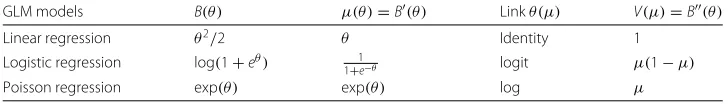
Different link functions will lead to different regression models as shown as in Table 1. Other GLMs such as negative binomial, gamma, and inverse Gaussian can be imple-mented accordingly with a differentV(μ). When dealing with big data problems with NP,whereNis the number of samples andPis the number of parameters, the inverse of aP×Pmatrix is time-consuming and computational challenging. We proposed an
Table 1Link functions for linear, logistic and Poisson regression models in GLM, where different models have differentA(∗),B(∗), andC(∗)
GLM models B(θ) μ(θ)=B(θ) Linkθ(μ) V(μ)=B(θ)
Linear regression θ2/2 θ Identity 1
Logistic regression log(1+eθ) 1+1e−θ logit μ(1−μ)
efficient algorithm to calculate the inverse of a much smallerN×N matrix as follows (Liu et al. 2015):
DXtVX+λIP×P
−1
DXt=DXtVXDXt+λIN×N
−1 .
So that whenNP, we have a much efficient estimation:
βnew=DXtVXDXt+λI−1 Z,
η=βold=βnew. (6)
The adaptive ridge algorithm (L0ADRIDGEA) is implemented in MATLAB are as follows:
TheL0ADRIDGE Algorithm: Given aλ >0,ε=1e−6, and training data{X,y},
Initializingβnew=rand(P, 1)/100, While 1,
η=βold=βnew, andD=diagη2 1,. . .,η2P
.
θ =Xβold,μ(θ)=G(θ)=B(θ), andY˜ =Y−μ(θ). V=diag[(B(θ1),. . .,B(θN)], andZ=VXβold+ ˜Y
IfN≥P,βnew =DXtVX+λI−1DXtZ, Else,βnew =DXtVXDXt+λI−1Z. if||βnew−η||< ε, Break; End End
The algorithm is easy to implement and very efficient for either small sample size and large dimension or large sample size and small dimension big data problem. The regular-ized parameterλcan be determined either by cross-validation or by AIC and BIC with
λ=2 andλ=log(N), respectively. We further discuss that the proposed method is aL0 approximation and converges toL0when the number of iterationsm→ ∞.
Algorithm justification: Given a high-dimensional big feature matrixXN×P(N P) and a threshold γ for the coefficient estimates,L0 rejects all the coefficient estimates belowγ to 0 and keeps the large coefficients unchanged. This is the same as defining a binary vectors =[. . ., 1, 0,. . ., 1]t, with the value of 0 or 1 for each feature, where sj = 1 if the coefficient estimate for that feature is above the thresholdγ, and 0 oth-erwise. LetS = diag(s)be a matrix withson its diagonal, we have the selected feature matrixXS = XS. We can build the standard models with the matrixXS, if we knowsin advance. For instance, we can estimate the coefficients of a GLM withL2regulation given XSandYwith
βnew=(Xt
SVXS+λI)−1XStZ=(XStVX+λI)−1XStZ=(SXtVX+λI)−1SXtZ, (7)
byDand a binarysjis approximated by a continuousηj2in proposed algorithm. Therefore, the proposed method is aL0approximation.
Recall the iterative system in Eq. (3), note that each feature is penalized by a differ-ent penalty, which is inversely proportional to the squared magnitude of that parameter estimatorηj. i.e.,
λj= λ
2η2j, and ηj=βj.
Smallerβj will lead to largerλj. A tinyβj, will become smaller andλjwill be getting larger in each iteration ofL0ADRIDGE algorithm.βj → 0, andλj → ∞. On the other hand, a largerβjwill lead a finiteλj, and nonzeroβj, when the number of iteration goes to∞. The solution ofL0ADRIDGE will converge to that of Eq. (7), because the effect of nonzeroηjwill be canceled out in Eq. (5). Note that our proposed methods will find a sparse solution with a large number of iterations and smallε, even though the solution ofL2regularized modeling is not sparse. Small parameters (βjs) become smaller at each iteration and will eventually go to zero (below the machine). We can also set a parameter to 0 if it is below predefinedε=1e−6 to speed up the convergence of the algorithm.
Results Simulations
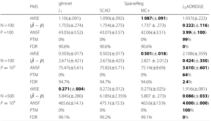
Poisson Regression: Our first simulation was used to evaluate the performance of our method for high dimensional Poisson regression. The data was generated from Pois-son distribution with different sample sizes (N) and dimensions (P). However, only features 1, 5, 10 and the constant term are used to generate the Poisson counts with [β0,β1,β5,β10]=[ 1, 0.5, 0.5, 0.4]. The countY is generated withY =Poisson(μ), where mean μ = exp(βX). The proposed method is compared with the glmnet ([16] and SparseReg package [17, 18]. glmnet and SparseReg implemented the elastic net, SCAD, and MC+ penalties with an efficient path algorithm. We compare the performance of our approach withL1(glmnet), SCAD and MC+ using the popular BIC (λ=log(N)) criteria. OurL0ADRIDGE is compared to the glmnet forL1and SparseReg for both SCAD and MC+. The results of different methods are presented in Table 2.
Table 2Performance of different GLM methods for Poisson regression over 100 simulations, where values in the parenthesis are the standard deviations, and ANSF: Average number of selected features; rMSE: Average square root of mean squared error;| ˆβ−β| = i| ˆβi−βi|: average absolute
bias when comparing true and estimated parameters
PMS glmnet SparseReg L0ADRIDGE
L1 SCAD MC+
rMSE 1.10(±.091) 1.090(±.092) 1.087(±.091) 1.937(±.222) N =100 | ˆβ−β| 1.755(±.274) 1.754(±.275) 1.737±.273) 0.222(±.116)
P =100 ANSF 43.03(±3.52) 43.07(±3.57) 42.06(±3.51) 3.99(±.100)
PTM 0% 0% 0% 99%
FDR 90.6% 90.6% 90.6% 0%
rMSE 0.503(±.017) 0.502(±.017) 0.501(±.018) 2.108(±.359) N =100 | ˆβ−β| 2.671(±.421) 2.673(±.425) 2.821±2.012) 0.424(±.350) P=103 ANSF 75.47(±5.61) 75.82(±5.71) 75.14(±8.69) 3.610(±.601)
PTM 0% 0% 0% 64%
FDR 94.7% 94.7% 94.6% 2.4%
rMSE 0.271(±.004) 0.272(±.012) 0.275(±.025) 1.916(±.081) N =500 | ˆβ−β| 5.845(±.280) 6.185(±2.359) 5.807±.273) 0.086(±.033) P=104 ANSF 465.6(±14.1) 475.1(±15.5) 463.6(±13.9) 4.000(±.000)
PTM 0% 0% 0% 100%
FDR 99.1% 99.2% 99.1% 0%
PMS: Performance Measures. PTM: Percentage of true models. FDR: False discovery rate. The values in boldface indicate the best performance
that both SCAD and MC+ can achieve a much smaller FDR, but a larger absolute bias and rMSE.
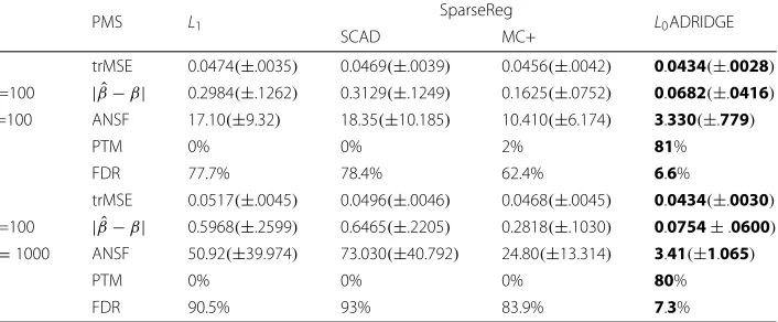
Logistic regression: The logistic regression data was generated with the coefficients of [β1,β5,β10]=[ 0.5, 0.5,−0.4], respectively, and the remaining coefficients were set to zero. The scorez=Xβ+ε, whereεis the random noise with the signal to noise ratio of 4. Then, the probabilityyis generated from the logistic functiony = 1/(1+e−z). Note thatyis the true probability instead of binary (1/0) in this simulation. Unlike the previous example, the optimal values ofλin this simulation were selected with the standard 5-fold cross-validation. We divided theλfromλmin=1e−4, toλmaxinto 100 equal intervals in log-scale, then chose the optimalλwith the smallest test error. The simulation was also repeated 100 times. The computational results were reported in Table 3. The values in the parenthesis are the positive/negative standard deviation.
Table 3Performance of different GLM methods for logistic regression over 100 simulations, where ANSF: Average number of selected features; trMSE: Test Average square root of mean squared error;
| ˆβ−β| = i| ˆβi−βi|: average absolute bias when comparing true and estimated parameters
PMS L1 SparseReg L0ADRIDGE
SCAD MC+
trMSE 0.0474(±.0035) 0.0469(±.0039) 0.0456(±.0042) 0.0434(±.0028)
N =100 | ˆβ−β| 0.2984(±.1262) 0.3129(±.1249) 0.1625(±.0752) 0.0682(±.0416)
P =100 ANSF 17.10(±9.32) 18.35(±10.185) 10.410(±6.174) 3.330(±.779)
PTM 0% 0% 2% 81%
FDR 77.7% 78.4% 62.4% 6.6%
trMSE 0.0517(±.0045) 0.0496(±.0046) 0.0468(±.0045) 0.0434(±.0030)
N =100 | ˆβ−β| 0.5968(±.2599) 0.6465(±.2205) 0.2818(±.1030) 0.0754±.0600) P=1000 ANSF 50.92(±39.974) 73.030(±40.792) 24.80(±13.314) 3.41(±1.065)
PTM 0% 0% 0% 80%
FDR 90.5% 93% 83.9% 7.3%
PMS: Performance Measures. PTM: Percentage of true models. FDR: False discovery rate. The values in boldface indicate the best performance
once, and MC+ only identified the true model 2 times for the dimension of 100, indicat-ing the super performance ofL0ADRIDGE under cross-validation. Finally,L0ADRIDGE is robust. The test square root of mean squared error and other performance measures did not vary much when the dimension increased from 100 to 1000. It is worth noting that our proposed method performs well with the popular statistical model selection cri-teria such as BIC and cross-validation. Other popular methods such asL1, SCAD, and MC+ select more features than necessary with such criteria. Therefore, many popular packages including the commercial MATLAB usually choose a largerλone standard devi-ation above the minimum test error with cross-validdevi-ation, which is arbitrary and leads to larger bias. To overcome such bias in parameter estimation, some packages re-estimate the parameters with the selected features and standard GLM model. Unlike these meth-ods, our proposed method performed much better without any postprocessing. Finally, the algorithm is very robust with different initialization. WithN = 100,P = 1000 and 100 times of different randomized initialization, we achieved the trMSE of 0.437(±.003), average absolute bias of 0.0763(±.07), ANSF of 3.39(±1.154), PTM of 85% and FDR of 6.9%, which is quite similar to the results with a fixed initialization.
TCGA ovarian cancer data
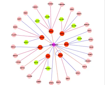
microRNA expression prediction with FPKM. FPKM, representing fragments per kilo-base of exon per million fragments mapped, measures the normalized read counts for RNA-seq. Three-fold cross validation was used for gene selection and validation. We reported the gene signatures with the best predicted area under the ROC curves (AUCs). Molecular signatures that are directly or indirectly associated with suboptimal debulking are shown in Fig. 1.
Figure 1 indicates that there are 16 gene signatures including 7 mRNAs and 9 epigenetic markers directly associated with debulking status. Even though there is no microRNA directly associated with debulking, eight microRNA signatures are indirectly associated with debulking through their association with mRNA signatures. Moreover, there are additional 18 epigenetic markers indirectly associated with debulking. The 7 mRNAs directly associated with debulking are EIF3D, PPP1R7, ADA, HSD17B1, SRBD1, ZNF621, and BARX1, where EIF3D, PPP1R7, BARX1 and ZNF621 have positive correlations and the other 3 genes have negative correlations with suboptimal debulking. Among the 7 mRNAs, ADA (Adenosine Deaminase) is a well-studied gene in ovarian neoplasms. ADA levels were found to be significantly higher in patients with ovarian cancers as compared with benign ovarian tumors [19]. ADA has been regarded as a potential biomarker for diagnosis and an agent for the treatment of ovarian cancer [20]. Other mRNAs such as BARX1, EIF3D, PPP1R7, and HSD17B1 are also known to be associated with differ-ent cancers or other diseases. At the microRNA level, there are 8 microRNAs indirectly associated with debulking including mir-183, let-7b, mir-9-1, mir-377, mir-202, mir-758,
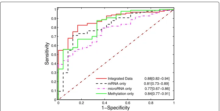
mir-375, and mir-30c-2. While let-7b, mir-30c-2, and mir-377 are positively correlated with suboptimal debulking through mRNAs ADA and BARX1 indirectly, the other 5 microRNAs have indirectly negative correlations with suboptimal debulking. Seven of eight microRNAs except for mir-758 are known to be associated with ovarian cancer. Particularly, let-7b is known to be an unfavorable prognostic biomarker and predict of molecular and clinical subclasses in high-grade serous ovarian carcinoma, and it may also be useful for discriminating between controls and patients with serous ovarian can-cer [21, 22]. Mir-183 is known to be associated with multiple cancan-cers. It regulates target oncogene (Tiam1), and reduce the migration, invasion and viability of ovarian cancer cells [23]. Finally, at the DNA level, nine epigenetically modified genes directly associ-ated with debulking are SSX1, TBR1, ZNF621, ORC3L, COL22A1, SPEF2, SSU72, EEF1D, and ZNF621, where EEF1D, SSU72, and ORC3L are positively associated with subopti-mal debulking, while 6 other epigenetic genes are negatively correlated with suboptisubopti-mal debulking. In addition, 18 other epigenetic genes indirectly associated with debulking may also have biological implications. Finally, integration of multi-omic data increases the prediction power substantially. Besides analyzing three types of omics data together, we performed the same three-fold cross validation for gene expression, methylation, and microRNA expression separately. The AUC curves are in Fig. 2.
Figure 2 shows that the best predicted AUC over 100 simulations for integrated data is 0.88, while the best predictive AUCs for gene expression, methylation, and microRNA over 100 simulations are 0.81, 0.84, and 0.76, respectively. The AUC with integrated data achieved the highest AUC, indicating the importance of multi-omics data mining. Genes selected with mRNA, microRNA, and methylations separately are reported in the sup-plementary document. In addition, we also compare the selected features and the same number of top genes identified with statistical test. The results are reported on Additional file 1: Table S2, and demonstrate that although individual genes are more statistically significant, combination of a panel of genes with standard logistic regression has less predictive power and test AUC (0.79).
0 0.2 0.4 0.6 0.8 1
0 0.1 0.2 0.3 0.4 0.5 0.6 0.7 0.8 0.9 1
1−Specificity
Sensitivity
Integrated Data 0.88[0.82−0.94] mRNA only 0.81[0.73−0.89] microRNA only 0.77[0.67−0.86] Methylation only 0.84[0.77−0.91]
Conclusions
Biomarkers from multi-omics data may predict disease status and help physicians to make clinical decisions.L0based GLM, which directly penalizes the number of nonzero parameters, has nice theoretical properties and leads to essential sparsity for biomarker discovery. Optimizing theL0regularization is a crucial, but difficult problem. We have developed an adaptive ridge algorithm (L0ADRIDGE) for approximatingL0 penalized GLM. The algorithm is easy to implement and efficient for problems with either an ultra-high dimension and small sample size, or a low-dimension and large sample size. It outperforms the other cutting edge regularization methods includingL1, SCAD and MC+ through simulations. When applied to the integration of multilevel omics data from TCGA and the prediction of suboptimal debulking from ovarian cancer, it can identify a panel of gene signatures achieving the best prediction power. We also demon-strate that prediction power of a model with multi-omics data increases substantially, when comparing with a model with one omics data, indicating the importance of big data mining.
Additional file
Additional file 1:Table S1. Performance of different GLM methods for Poisson regression over 100 simulations, where values in the parenthesis are the standard deviations, and ANSF: Average number of selected features; rMSE: Average square root of mean squared error;| ˆβ−β| = i| ˆβ−βi|: average absolute bias when comparing true and
estimated parameters. PMS: Performance Measures. PTM: Percentage of true models. FDR: False discovery rates. The L0ADRIDGE is compared to the best performance chosen fromλ=0.9λmaxandλ=0.5λmaxwith both for SCAD and
MC+. Table S2. The comparison of performance of the our sparse modeling approach and the top genes selected with Student’s t-test. The results demonstrate that although each gene is more statistically significant with statistical test, the combination of the panel of genes has less predictive power and test AUC with standard logistic regression and three-fold cross valida- tion, indicating the collinearity among theses genes. (PDF 86 kb)
Abbreviations
AUC: The area under an ROC curve; GLM: Generalized linear model;L0ADRIDGE:L0adaptive ridge algorithms; MC+:
Minimax concave penalty. SCAD: Smoothly clipped absolute deviation; TCGA: The cancer genome atlas
Acknowledgements
This work was partially supported by the DMS-1343506 grant from the National Science Foundation (ZL), and P01 CA098912-10 and UL1 TR0001881-01 grants from NIH. The funders had no role in the preparation of the article.
Funding
DMS-1343506 of NSF (ZL), P01 CA098912-10 and UL1 TR0001881-01.
Availability of data and materials
L0ADRIDGE in MATLAB is available at https://github.com/liuzqx/L0adridge.
Authors’ contributions
ZL conceptualized and designed method, developed the software, and wrote the manuscript. SF, MDP helped in method design and manuscript writing and revised the manuscript critically. All authors read and approved the final manuscript.
Ethics approval and consent to participate Not Applicable.
Consent for publication Not Applicable.
Competing interests
The authors declare that they have no competing interests.
Publisher’s Note
Springer Nature remains neutral with regard to jurisdictional claims in published maps and institutional affiliations.
Author details
1Samuel Oschin Comprehensive Cancer Institute, Cedars-Sinai Medical Center, Los Angeles 90048, CA, USA.2Molecular
and Computational Biology Program, Department of Biological Sciences, University of Southern California, Los Angeles 90089, CA, USA.3Foundation Inflammatory Bowel & Immunobiology Research Institute, Cedars-Sinai Medical Center, Los
Received: 13 April 2017 Accepted: 4 December 2017
References
1. Tibshirani R. Regression shrinkage and selection via the lasso. J Roy Stat Soc B. 1996;58:267–88. 2. Zou H. The adaptive lasso and its oracle properties. J Am Stat Assoc. 2006;101:1418–29.
3. Lin D, Foster D, Ungar L. A risk ratio comparison of l0 and l1 penalized regressions. Tech. rep., University of Pennsylvania; 2010.
4. Kakade S, Shamir O, Sridharan K, Tewari A. Learning exponential families in high dimensions: strong convexity and sparsity. JMLR. 2013;9:381–8.
5. Bahmani S, Raj B, Boufounos P. Greedy sparsity-constrained optimization. J Mach Learn Res. 2013;14(3):807–41. 6. Zhang T. Multi-stage convex relaxation for feature selection. Bernoulli. 2012;19:2153–779.
7. Fan J, Li R. Variable selection via nonconcave penalized likelihood and its oracle properties. J Am Stat Assoc. 2001;96:1348–61.
8. Zhang C. Nearly unbiased variable selection under minimax concave penalty. Ann Stat. 2010;38:894–942. 9. Liu Z, Lin S, Deng N, McGovern D, Piantadosi S. Sparse inverse covariance estimation with L0 Penalty for Network
Construction with Omics Data. J Comput Biol. 2016;23(3):192–202.
10. Liu Z, Li G. Efficient Regularized Regression withL0Penalty for Variable Selection and Network Construction. Comput Math Methods Med. 2016;2016:3456153.
11. Bahmani S, Boufounos P, Raj B. Learning Model-Based Sparsity via Projected Gradient Descent. IEEE Trans Info Theory. 2016;62(4):2092–9.
12. Riester M, Wei W, Waldron L, Culhane A, Trippa L, Oliva E, Kim S, Michor F, Huttenhower C, Parmigiani G, Birrer M. Risk prediction for late-stage ovarian cancer by meta-analysis of 1525 patient samples. J Natl Cancer Inst.
2014;106(5): Apr 3.
13. Tucker S, Gharpure K, Herbrich S, Unruh A, Nick A, Crane E, Coleman R, Guenthoer J, Dalton H, Wu S, Rupaimoole R, Lopez-Berestein G, Ozpolat B, Ivan C, Hu W, Baggerly K, Sood A. Molecular biomarkers of residual disease after surgical debulking of high-grade serous ovarian cancer. Clin Cancer Res. 2014;20(12):3280–8. 14. Liu Z, Beach J, Agadjanian H, Jia D, Aspuria P, Karlan B, Orsulic S. Suboptimal cytoreduction in ovarian carcinoma
is associated with molecular pathways characteristic of increased stromal activation. Gynecol Oncol. 2015;139(3): 394–400.
15. Wood S. Generalized Additive Models: An Introduction with R. New York: Chapman & Hall/CRC; 2006.
16. Friedman J, Hastie T, Tibshirani R. Regularization Paths for Generalized Linear Models via Coordinate Descent. J Stat Softw. 2011;33(1):1–22.
17. Zhou H, Lange K. A path algorithm for constrained estimation. J Comput Graph Stat. 2013;22(2):261–83.
18. Zhou H, Wu Y. A generic path algorithm for regularized statistical estimation. J Am Stat Assoc. 2014;109(506):686–99. 19. Urunsak I, Gulec U, Paydas S, Seydaoglu G, Guzel A, Vardar M. Adenosine deaminase activity in patients with
ovarian neoplasms. Arch Gynecol Obstet. 2012;286(1):155–9.
20. Shirali S, Aghaei M, Shabani M, Fathi M, Sohrabi M, Moeinifard M. Adenosine induces cell cycle arrest and apoptosis via cyclinD1/Cdk4 and Bcl-2/Bax pathways in human ovarian cancer cell line OVCAR-3. Tumour Biol. 2013;34(2):1085–95.
21. Tang Z, Ow G, Thiery J, Ivshina A, Kuznetsov V. Meta-analysis of transcriptome reveals let-7b as an unfavorable prognostic biomarker and predicts molecular and clinical subclasses in high-grade serous ovarian carcinoma. Int J Cancer. 2014;134(2):306–18.
22. Chung Y, Bae H, Song J, Lee J, Lee N, Kim T, Lee K. Detection of microRNA as novel biomarkers of epithelial ovarian cancer from the serum of ovarian cancer patients. Int J Gynecol Cancer. 2013;23(4):673–9.
23. Li J, Liang S, Jin H, Xu C, Ma D, Lu X. Tiam1, negatively regulated by miR-22, miR-183 and miR-31, is involved in migration, invasion and viability of ovarian cancer cells. Oncol Rep. 2012;27(6):1835–42.
• We accept pre-submission inquiries
• Our selector tool helps you to find the most relevant journal • We provide round the clock customer support
• Convenient online submission • Thorough peer review
• Inclusion in PubMed and all major indexing services • Maximum visibility for your research
Submit your manuscript at www.biomedcentral.com/submit