www.the-cryosphere.net/10/1947/2016/ doi:10.5194/tc-10-1947-2016
© Author(s) 2016. CC Attribution 3.0 License.
A model for the spatial distribution of snow water equivalent
parameterized from the spatial variability of precipitation
Thomas Skaugen1and Ingunn H. Weltzien1,2,a
1Norwegian Water Resources and energy Directorate, P.O. Box 5091, Maj. 0301 Oslo, Norway 2Department of Geosciences, University of Oslo, Oslo, Norway
anow at: Norconsult AS, P.O. Box 626, 1303, Sandvika, Norway Correspondence to:T. Skaugen ([email protected])
Received: 10 February 2016 – Published in The Cryosphere Discuss.: 19 February 2016 Revised: 12 August 2016 – Accepted: 22 August 2016 – Published: 6 September 2016
Abstract.Snow is an important and complicated element in hydrological modelling. The traditional catchment hydrolog-ical model with its many free calibration parameters, also in snow sub-models, is not a well-suited tool for predicting conditions for which it has not been calibrated. Such con-ditions include prediction in ungauged basins and assessing hydrological effects of climate change. In this study, a new model for the spatial distribution of snow water equivalent (SWE), parameterized solely from observed spatial variabil-ity of precipitation, is compared with the current snow distri-bution model used in the operational flood forecasting mod-els in Norway. The former model uses a dynamic gamma dis-tribution and is called Snow Disdis-tribution_Gamma, (SD_G), whereas the latter model has a fixed, calibrated coefficient of variation, which parameterizes a log-normal model for snow distribution and is called Snow Distribution_Log-Normal (SD_LN). The two models are implemented in the param-eter parsimonious rainfall–runoff model Distance Distribu-tion Dynamics (DDD), and their capability for predicting runoff, SWE and snow-covered area (SCA) is tested and compared for 71 Norwegian catchments. The calibration pe-riod is 1985–2000 and validation pepe-riod is 2000–2014. Re-sults show that SD_G better simulates SCA when compared with MODIS satellite-derived snow cover. In addition, SWE is simulated more realistically in that seasonal snow is melted out and the building up of “snow towers” and giving spuri-ous positive trends in SWE, typical for SD_LN, is prevented. The precision of runoff simulations using SD_G is slightly inferior, with a reduction in Nash–Sutcliffe and Kling–Gupta efficiency criterion of 0.01, but it is shown that the high
preci-sion in runoff prediction using SD_LN is accompanied with erroneous simulations of SWE.
1 Introduction
Snow is an important hydrological parameter in the North-ern Hemisphere and in Norway approximately 30 % of the annual precipitation falls as snow. Snow and snow-related hydrology have a significant impact on nature and society in such regions. Seasonal snow ensures variation in outdoor activities and considerable investments in infrastructure for tourism and hydropower are dependent on stable seasonal snow. Apart from snow-related hazards such as spring melt floods and avalanches, snow may negatively affect construc-tion safety and traffic flow at airports, roads and in urban ar-eas. Information about snow conditions at the local, regional and national scale is therefore important for the early warn-ing of hazards, as well as for tourism, hydropower production planning and water resources management.
res-olution; Anderson, 1976) and for stationary climatic condi-tions. Another reason is that hydrological snow models are expected to provide simulations at the catchment scale, for which there are usually no estimates of more nonstandard hydrological model forcing such as, for example, wind and radiation. In addition, the governing equations for the physics of hydrology at the small scale have proven difficult to scale up in time and space to be relevant for catchment hydrology (Kirchner, 2006).
For predictions in ungauged basins and in a changed cli-mate, however, calibrated empirical relations in snow mod-els cannot be expected to give reliable and useful results. Skaugen et al. (2015) used the Distance Distribution Dynam-ics (DDD) model (Skaugen and Onof, 2014) for prediction in ungauged basins with model parameters estimated from catchments characteristics. When analysing the deviations in performance between the calibrated and the regionalized ver-sions of the DDD model, the regionalized degree-day fac-tor for snowmelt and the coefficient of variation (CV) for the spatial probability density function (PDF) of snow water equivalent (SWE) emerged as the parameters most responsi-ble for poor regionalized results for runoff.
A realistically modelled spatial PDF of SWE is impor-tant for the temporal evolution of SWE, snowmelt and snow-covered area (SCA) (Buttle and McDonnel, 1987; Liston, 1999; Luce et al., 1999; Essery and Pomeroy, 2004; Luce and Tarboton, 2004). In the literature, many models for the PDF are proposed, especially for the period of time of maximum accumulation, such as the log-normal distribu-tion (Donald et al., 1995, Sælthun, 1996), the gamma dis-tribution (Kutchment and Gelfan, 1996; Skaugen, 2007; Kol-berg and Gottschalk, 2010; Skaugen and Randen, 2013) and the normal distribution (Marchand and Killingtveit, 2004, 2005). Helbig et al. (2015) investigated the spatial PDF of snow depth for three large alpine areas and found that the gamma and the normal distributions were better suited than the log-normal distribution. In Alfnes et al. (2004), Skau-gen (2007) and SkauSkau-gen and Randen (2013), it was demon-strated through the repeated measurements of the same snow course during the accumulation and melting seasons that the spatial PDF of SWE changed its shape continuously during the periods of accumulation and melting. During the accu-mulation period, the spatial distribution of SWE would be-come less positively skewed as accumulation progressed and increasingly more positively skewed as melting progressed. Good simulation of the evolution of SCA is especially im-portant since it controls the runoff dynamics of the spring melt flood and is the basis for properly accounting the energy fluxes in land-surface schemes in atmospheric models (Lis-ton, 1999; Essery and Pomeroy, 2004; Helbig et al., 2015).
In this study we will test an alternative method for param-eterizing the spatial PDF of SWE. In the alternative method the spatial PDF of SWE is modelled as a dynamic gamma distribution and is hereafter denoted SD_G (Snow Distribu-tion_Gamma). The parameters of SD_G are estimated solely
from observed spatial variability of precipitation; i.e. all its parameters are estimated prior to the calibration of the hydrological model against runoff. Information on the spa-tial variability of precipitation is available at many sites, which makes it possible to use the method for prediction in ungauged basins. Downscaled climate changes projections may also provide such information so that effects of climate change on snow conditions and hydrology may be assessed. In using such a method, the current dependency of calibra-tion in hydrological snow models is reduced.
SD_G is described in Skaugen (2007) and has since been developed in Skaugen and Randen (2013). The method was tested at small test sites and found to model the spatial mo-ments of SWE and SCA well (Skaugen and Randen, 2013) but has, however, not been implemented in a hydrological model and hence not been tested for larger scales and as a tool in operational hydrology. In this study, the SD_G is im-plemented in the DDD model and its performance is com-pared with the currently used snow distribution model, the Snow Distribution_Log-Normal (SD_LN) (Killingtveit and Sælthun, 1995; Sælthun, 1996). SD_LN distributes SWE log normally in space with a fixed, calibrated CV. It has been used operationally in Norwegian hydrology for many years, although it has the feature of being a calibrated model and hence not suitable for climate change studies and for predic-tions in ungauged basins. In addition, a fixed CV, and hence an assumption of perfect spatial correlation, is not supported by observations (Alfnes et al., 2004), and in a recent paper Frey and Holzmann (2015) show that a log-normal spatial distribution of SWE with a fixed CV of introduces so-called “snow towers”. For high-elevation areas, and for the highest quantiles of the distribution, snow survived the summer and accumulated to give an overall positive trend in SWE, which was not observed.
The main objective of this paper is to evaluate if SD_G is a suitable alternative for use in rainfall–runoff models. We will compare simulated results of runoff, SWE, SCA and snow cover duration simulated with DDD using the current model, SD_LN, and with the alternative, SD_G, for 71 catch-ments in Norway. Time series of satellite-derived SCA from MODIS (Moderate Resolution Imaging Spectroradiometer) images are available for the catchments, so simulated runoff and SCA will also be compared against observed values.
2 Method
subsec-tion describes howE(Z0)and Var(Z0)are estimated for ac-cumulation and melting events. Acac-cumulation and melting events may change the spatial extent of SCA, which will re-quire special consideration when estimating the E(Z0)and Var(Z0). In this study SCA is set equal to 1 (full coverage) for every snowfall event, whereas a melting event implies a reduction in coverage. With estimates ofE(Z0)and Var(Z0), the parameters of the gamma distributions are calculated as
ν= E(Z
0)2
Var(Z0) (1a)
andα= E(Z
0)
Var(Z0). (1b)
In the first subsection, the model for estimating the statis-tical moments,E(Z0)and Var(Z0), for the accumulated sum of SWE,Z0, is presented. As in Skaugen and Randen (2013), the moments are derived from the sum of correlated gamma distributed unit fields,y(x)[mm], wherexrepresents space. For the remainder of the paper the unit field,y (x), is denoted
y.
Section 2.1.1–2 briefly address the estimation of E(Z0)
and Var(Z0) for accumulation and melting events with a changing SCA. The derivation for accumulation events dif-fers from that presented in Skaugen and Randen (2013) and is presented in detail. For melting events, however, only the resulting equations are presented since the full derivations can be found in Skaugen and Randen (2013).
Section 2.2 describes how change in SCA is estimated af-ter a melting event and Sect. 2.3 describes briefly the hydro-logical model and its current model for the spatial distribu-tion of SWE, SD_LN.
The final subsection, Sect. 2.5, describes the procedure for testing and comparing the new model for the spatial distri-bution of SWE, SD_G against the current, SD_LN. The data used will also be presented here.
2.1 Statistical moments of spatial SWE
The PDF of Z0 does not contain zeros and is hence condi-tional on snow. For the non-condicondi-tional distribution of SWE, which also includes zeros, the variable SWE is denotedZ. The unit fields of snowfall are distributed in space according to a two-parameter gamma distribution, y=G(ν0α0), with PDF:
f (y)= 1
0(ν0)
αν0
0 y
ν0−1e−α0yα
0ν0y >0, (2) where 0 is the gamma function and α0 and ν0 are shape and scale parameters respectively. The mean of the unit equals E (y)=ν0/α0 and the variance equals Var(y)=
ν0/α20. When estimating the moments for the sum ofnunits,
Z0(n)=
n
P
i=1
yi, we have to take into account that the unit fields are correlated. This has no bearing on the mean,E(Z0), but affects the variance, Var(Z0), i.e.
E Z0=nν0 α0
=ν
α, (3)
Var Z0=nν0 α20
+2X
i<jCov(yi, yj)
=nν0 α02[1
+(n−1) c (n)]= ν
α2, (4)
where the function c(n) is the average correlation over n
units.
From Eq. (4) we see that if we have perfect and con-stant correlation between they’s,c(n)=1, the variance of
Z0equals Var(Z0)=n2ν0
α2 0
. From Eqs. (3) and (4)we see that the relationship between the standard deviation,σZ0, and the
mean, E(Z0), is a straight line with slope equal to ν0−0.5,
σZ0=ν−0.5
0 E Z
0
. However, if we have no correlation be-tween they’s,c(n)=0, the variance equals Var(Z0)=nν0
α2 0
, which gives a relationship between σZ0 and E(Z0) as a
curved line that departs from that of perfect correlation by
n−0.5,σZ0=(ν0n)−0.5E(Z0). The variance, however, is
lin-early related to the mean. Correlation between the units,c(n), gives a relationship between the mean and the standard de-viation that is something between the two cases described above. A typical analytical approximation to the spatial and temporal correlation function for precipitation is an exponen-tially decaying function with either time or space as argu-ment. Zawadski (1973, 1987) found exponential decorrela-tion for rainfall for both time and space. Asn(number of summations) may be considered a variable akin to time,c(n)
is approximated by an exponential correlation function:
c(n)=exp(−n
D), (5)
whereDis the decorrelation range in which the correlation equals 1/e(Zawadski, 1973).
The variance ofZ can now, with Eqs. (4) and (5), be ex-pressed as
Var Z0=E(Z0)1 α0
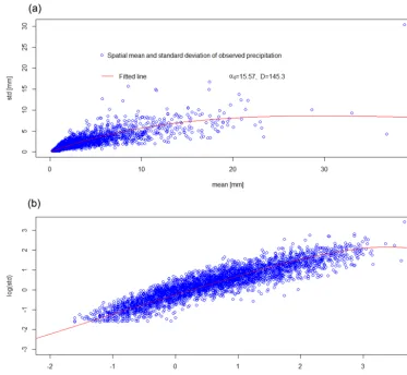
Figure 1.Scatter plot of the spatial mean and spatial standard deviation of observed precipitation over a catchment. Equation (6) is fitted to the data by nonlinear regression (red line). Bottom panel shows the scatter plot in log–log.
The parametersa0,ν0andDare estimated from an analy-sis of the variability of precipitation as shown in Fig. 1 for the catchment of interest. A mean of the units has been chosen as E (y)=ν0
α0 =0.1 mm, since 0.1 mm is the smallest
pre-cipitation value measured by the Norwegian Meteorological Institute.
2.1.1 Statistical moments of spatial SWE after an accumulation event
From a single snowfall event ofnunits on a snow-free sur-face, the mean and the variance of the snow reservoirZ are estimated according to Eqs. (3) and (4). If there is an addi-tional snowfall event of u units, the mean of the resulting snow reservoir is
E Zn+u0=(n+u)
a0
ν0
, (7)
and the variance is
Var Zn+u0
= ν
α2+u
ν0
α02
[1+(u−1) c (u)], (8) where ν
α2 is the conditional variance prior to the
accumula-tion event. In order to keep the notaaccumula-tion simple we say thatn
is the number of units att−1 anduis the number of units of the event at timet.
Equations (7) and (8) are valid if SCA=1 for both events. If SCA prior to the new event was reduced due to melting (SCAt−1<1), we have to scale the contributions ofnandu according to the change in SCA from SCAt−1<1 to SCAt= 1; hence the mean is
E Zn+u0=
a0
ν0
(SCAt−1(n+u)+SCAtu) , (9) and the variance is
Var Zn+u0=SCA2t−1(
ν α2+u
ν0
α02([1
+(u−1) c (u)]))
+SCA2t ν0
α20u ([1
2.1.2 Statistical moments of spatial SWE after a melting event
Let the snow reservoir, consisting ofnunits, be reduced byu
units after a melting event. The snow coverage before and after the melting event is SCAt−1 and SCAt respectively, where SCAt<SCAt−1. We set SCAt−1as 1, so that SCAt is the relative reduction in snow coverage due to melting, and not the catchment value. Reduction in snow coverage needs special attention regarding the conditional (Z0) and the non-conditional (Z)moments since we have to determine the spatial moments for the area of the new coverage, SCAt (not including zeros, i.e. conditional moments) and for the area which includes the previously covered part, SCAt−1 (includ-ing zeros, i.e. non-conditional moments).
The non-conditional mean after the melting event is esti-mated as
E (Zn−u)=(n−u)
ν0
α0
, (11)
and the conditional mean is
E Zn−u0=
E (Zn−u) SCAt
= 1
SCAt
(n−u)ν0 α0
. (12)
We note that the difference in conditional means before and after the melting event is
E(Z0n)−E(Z0n−u)=
ν0
α0
n−(n−u) 1
SCAt
=ν0
α0
u0, (13)
whereu0 is the conditional number of melted units and de-scribes the difference in units when the (relative) reduction in SCA is taken into account.
Skaugen and Randen (2013) give a detailed derivation of the conditional spatial variance of SWE after a melting event. Here, only the final expression is reported:
Var Zn−u0=
ν α2−2u
0 nν0
α02cmlt u 0
+u0ν0 α02
+u0(u0−1)ν0 α02c(u
0
), (14)
where ν
α2 is the variance ofZ
0prior to the melting event, and cmlt u0is the (negative) correlation between melt and SWE and is estimated as a linearly decreasing function of uand equal to
cmlt u0=
u0 n
1 2n
ν α2
α02 nν0
+1+(n−1) c (n) !!
. (15)
It is clear from Eq. (13) that estimation of the change in SCA due to melting is needed in order to assessuand con-sequently Var Zn−u0
in Eq. (14). The next subsection de-scribes such a procedure.
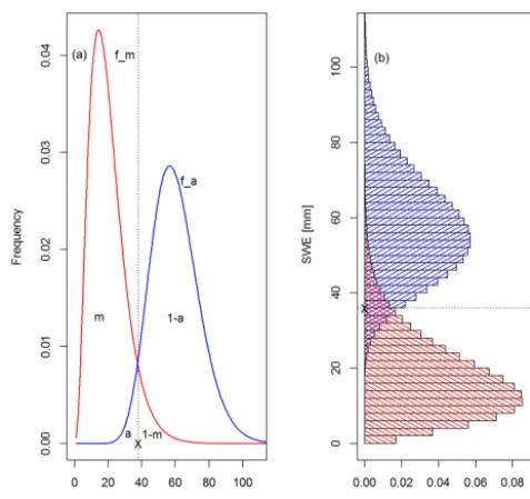
Figure 2.Schematic of how changes in SCA are estimated.(a)fm andfa are the spatial frequency distributions (PDF) of snowmelt and accumulation respectively.m, 1−m,aand 1−aare partially integrated values of the PDFs.(b)The integral of the PDFs for suc-cessive intervals of SWE and melt and their spatial coverage. The cross-hatched bars constitute the reduction in SCA.
2.2 Estimating changes in snow-covered area
After a snowfall event, the SCA for the area of interest (a catchment or a part of a catchment in the case of eleva-tion bands) is set equal to 1. For a melting event, however, the estimate of changes in SCA is more complex. The pre-vious subsection suggests modelling the accumulated SWE as a gamma distribution,fa, with parameters ν andα de-rived from the estimated mean and variance of accumulated SWE as described above. In Skaugen and Randen (2013), the spatial frequency of snowmelt, fm, was also modelled as a gamma distribution following the same principles as for accumulation, i.e. that the moments can be estimated using Eqs. (3) and (4) withureplacingn. At all timesu0≤n, which implies that until the final melting event occurs,fmis more skewed to the left thanfa.
integral offmup to X, calledm,R0Xfm=min the Fig. 2a and much larger than the area of SWE values less thanX(the integral offaup toX, calleda, isR0Xfa=ain Fig. 2a). Con-sequently, the fractional area of SWE values less thanX,a, becomes snow free after the melting event. In addition, there are melt values higher than X that reduce the coverage of corresponding SWE values. The sum of these bars adds up to 1−mand equals the integralR∞
X fm=1−m. In total, the reduction of SCA after a melting event is
SCAred=a+1−m (16)
and is seen in Fig. 2b as the sum of the cross-hatched bars. Recall that the reduction in SCA is relative; i.e. it is the re-duction from the previous snow cover, which is also the prob-ability space of bothfaandfmand equal to 1.
The correlation of snowmeltc(u)as a function of intensity (u)(see Eq. 14) has not yet been investigated in detail and is, in this study, modelled as that of accumulation. Skaugen and Randen (2013), however, reported empirical evidence sup-porting such an assumption. The observed features offmare found to be similar to those offa, i.e. that the spatial distribu-tion is generally skewed to the left and becomes less skewed as the intensity of melt increases. These features for fmare confirmed by additional measurements of spatial snowmelt by Weltzien (2015).
2.3 The hydrological model
The DDD model (Skaugen and Onof, 2014; Skaugen et al., 2015; Skaugen and Mengistu, 2015) is a rainfall– runoff model written in the programming language R (www. r-project.org) and runs operationally at daily and 3-hourly time steps at the Norwegian flood forecasting service at the Norwegian Water Resources and Energy Directorate (NVE). The DDD model introduces new concepts in its description of the subsurface and of runoff dynamics and is developed with the objective of having as many as possible of its model parameters estimated directly from observed data such as maps and runoff characteristics and not through calibration against runoff. In its current version, the parameters of the modules for subsurface and runoff dynamics are all estimated prior to calibration against runoff. Input to the DDD model is precipitation and temperature. The model is semi-distributed in that the moisture-accounting (rainfall and the accumulat-ing and meltaccumulat-ing of snow) is performed for 10 elevation bands of equal area. The catchment averages of precipitation and temperature are distributed to the elevation bands using cali-brated lapse rates. The catchment averaged precipitation can be corrected by multiplying the amount with a constant in order to get the long-term water balance right. Snowmelt is estimated using a degree-day model (Ohmura, 2001; Hock, 2005), where the melted amount is a linear function of the difference between actual air temperature and a calibrated threshold temperature for melting. In the current routine in DDD for the spatial PDF of SWE (SD_LN), the PDF is
mod-elled as the sum of uniform and log-normally distributed snowfall events (Killingtveit and Sælthun, 1995; Sælthun, 1996). The distribution is constant for up to a specified threshold of accumulated SWE (i.e. 20 mm). Each additional snowfall event is log-normally distributed through a cali-brated coefficient of variation,θCV, and SWE is estimated for nine quantiles and added to previous quantile values. In this way, each additional snowfall event has a spatial distribution of a fixed shape (through the calibratedθCV)regardless of its intensity. Moreover, the method implies perfect spatial corre-lation in that a new snowfall is distributed such that the quan-tiles with highest SWE always receives most SWE so that the CV of the sum of snowfall events remains a constant. A sim-ple examsim-ple demonstrates this: if the accumulation of SWE,
Z, is the sum of two snowfall eventsy,Z=y1+y2, where
y∼LN(µy, σy2)is log-normally distributed with mean µy and varianceσy2, then the mean of Z is E (Z)=2µy and the variance is Var(Z)=σy2+σy2+2COV(y1, y2). With per-fect correlation the variance equals Var(Z)=σy2+σy2+2σy2
(Haan, 1977, p. 56) and it is easily seen that the CV forZ
equals that ofy, i.e.
CVZ=
σZ
µZ
= 2σy
2µy
=CVy. (17)
The spatial distribution of melt is constant and reduction in SCA occurs when the SWE associated with a quantile be-comes 0. The fraction of snow-free areas is thus the sum of quantiles with zero SWE.
The model parameters relevant for snow accumulation and melt which are estimated by calibration against runoff in-cludeθCV, describing the spatial distribution of SWE,θCX, which is the degree-day factor, andθWs, which is the max-imum liquid water content in the snowpack (see Table 1 of model parameters).
Further details on the DDD model are found in Skau-gen and Onof (2014) and in SkauSkau-gen and Mengistu (2015). Model parameters that can be calibrated against runoff are denoted byθwith subscripts (e.g.θCV)in order to clearly dis-tinguish between estimated and calibrated parameters. From Table 1 we see that 11 model parameters have the potential to be calibrated. The next subsection shows, however, that the number of calibrated parameters for this study is reduced to five (shown in bold in Table 1).
2.4 Test of SD_G in DDD
We will evaluate the performance of SD_G, parameterized from observed spatial variability of precipitation, by imple-menting it in DDD (DDD_G) and compare performance with DDD_LN, in which SD_LN, with its calibration parameter
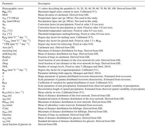
Table 1.Parameters of the DDD model with description and method of estimation. Some parameters (denoted with a∗) have values obtained through experience in calibrating DDD for gauged catchments in Norway. These values are within the recommended range for the HBV model (Sælthun, 1996). Other parameter values are assigned standard values as suggested in the literature. The GIS analyses are carried out using the national 25×25 m digital elevation model (http://www.statkart.no). Parameters in bold have been calibrated in this study, by either dataset V1 or V2.
Parameter Description
Hypsographic curve 11 values describing the quantiles 0, 10, 20, 30, 40, 50, 60, 70, 80, 90, 100. Derived from GIS.
θWs[%] Maximum liquid water content in snow. Calibrated (V1).
Hfelt Mean elevation of catchment. Derived from GIS.
θTlr[◦C/100 m] Temperature lapse rate (pr 100 m). Not used in this study.
θPlr[mm/100 m] Precipitation lapse rate (pr 100 m). Not used in this study.
θPc Correction factor for precipitation. Fixed at value 1.0 (see text).
θSc Correction factor for precipitation as snow. Fixed at value 1.0 (see text).
θTX[◦C] Threshold temperature rain/snow. Fixed at value 0.5 (see text).
θTS [◦C] Threshold temperature melting/freezing. Fixed at value 0.0 (see text).
θCX[mm◦C−1day−1] Degree-day factor for melting snow. Calibrated (V2). ∗C
Glac[mm◦C−1day−1] Degree-day factor for glacial melt. Fixed at value 1.5×θCX. ∗
CFR [mm◦C−1day−1] Degree-day factor for refreezing. Fixed at value 0.02.
Area [m2] Catchment area. Derived from GIS.
maxLbog [m] Maximum of distance distribution for bogs. Derived from GIS.
midLbog [m] Mean of distance distribution for bogs. Derived from GIS.
Bogfrac Fraction of bogs in catchment. Derived from GIS.
Zsoil Areal fraction of zero distance to the river network for soils. Derived from GIS.
Zbog Areal fraction of zero distance to the river network for bogs. Derived from GIS.
NOL Number of storage levels. Fixed at value 5 (Skaugen and Onof, 2014).
θcea[mm◦C−1day−1] Degree-day factor for evapotranspiration. Calibrated (V1).
R Parameter defining field capacity (Skaugen and Onof, 2014).
δ Shape parameter of gamma distributed recession characteristic. Estimated from recession.
β Scale parameter of gamma distributed recession characteristic. Estimated from recession.
θCV Coefficient of variation for spatial distribution of snow. Calibrated (V2).
α0 Scale parameter of unit precipitation. Estimated from observed spatial variability of precipitation.
D Decorrelation length of spatial precipitation. Estimated from observed spatial variability of precipitation.
θmat hbf vr[m s−1] Mean celerity in river. Calibrated from (V1).
mRd[m] Mean of distance distribution of the river network. Derived from GIS.
sRd[m] Standard deviation of distance distribution of the river network. Derived from GIS.
Rdmax[m] Maximum of distance distribution in river network. Derived from GIS.
mS[mm] Mean of subsurface water reservoir. Estimated from recession.
d[m] Mean of distance distribution for hillslope. Derived from GIS.
dmax[m] Maximum of distance distribution for hillslope. Derived from GIS.
Glacfrac Fraction of bogs in catchment. Derived from GIS.
mGl[m] Mean of distance distribution for glaciers. Derived from GIS.
sGl[m] Standard deviation of distance distribution for glaciers. Derived from GIS.
Areal fraction of glaciers in 10 elevation zones
Derived from GIS.
the Norwegian Meteorological Institute, are daily precipita-tion values from precipitaprecipita-tion gauges (a minimum of two sta-tions) located close to the catchment in question and are from the period 1990–2011.
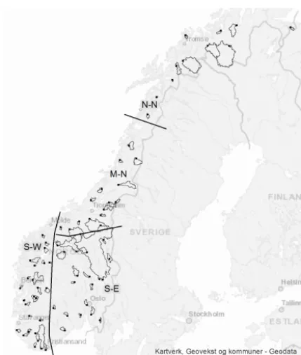
DDD_G and DDD_LN are run for 71 catchments dis-tributed across Norway (see Fig. 3). The catchments vary in latitude, size, elevation and surface cover (see histograms of selected catchment characteristics (CC) in Fig. 4) and consti-tute thus a varied, representative sample of Norwegian catch-ments. The runoff data are provided by NVE and we use the period of 1 September 1985 to 31 August 2000 for
calibra-tion of DDD_G and DDD_LN and the period of 1 Septem-ber 2000 to 31 DecemSeptem-ber 2014 for validation.
Figure 3.Location of the 71 catchments used to evaluate the new subsurface routine. The results presented in the next section are or-ganized with respect to the regions south-east E), south-west (S-W), mid-Norway (M-N) and Northern Norway (N-N).
grid was developed, denoted V2 (Lussana et al. 2014a, b), which reduced much of the positive bias in precipitation characteristic of V1 (see Saloranta, 2012). The new meteo-rological grid (V2) in DDD gives reasonable simulated val-ues of runoff without the need for a calibrated correction of the amount of precipitation (θPc; see Table 1 for parameters of the DDD model). Areal averages of precipitation and tem-perature values are extracted for 10 elevation zones, which makes it possible to eliminate calibrated precipitation and temperature gradients (θPlrandθTlr). Three parameters asso-ciated with snow accumulation and melt – the correction fac-tor for solid precipitation (θSc=1.0), the threshold tempera-ture for snowmelt (θTs=0◦C) and the threshold temperature for solid and liquid precipitation (θTX=0.5◦C) – were fixed, thereby reducing the number of calibration parameters from 11 to 5. For the remaining five parameters, the calibrated val-ues (from using V1 as input) are retained for three parameters (θWs,θvrandθcea), whereas for the DDD_LN model,θCXand
the parameter of interest for this study,θCV, are recalibrated using V2 as input data. In using such a procedure we assume that the three parameters which are calibrated using the V1 data (and, most likely, not optimal using the V2 data as input) will not favour either of the two compared model structures (DDD_LN and DDD_G). When recalibrating the θCVwith V2 data, we attempt to make it as difficult as possible to ac-cept the new spatial frequency distribution of SWE (SD_G). If we calibrated all three parameters (θWs,θvr andθcea)using
V2, we could risk that errors associated with the structures of SD_G and SD_LN were compensated by the other three parameters, such that we could not isolate and evaluate the effect of implementing SD_G. In addition, for the DDD_G model, the degree-day factorθCXwas calibrated since corre-lation between this parameter andθCVwas revealed. It would hence be probable that aθCX optimized using SD_LN with V1 would not be optimal for testing SD_G.
From almost 1500 optical satellite scenes from MODIS during the period 2001–2015, SCA for each elevation band have been estimated for 69 of the 71 catchments (for two of the catchments SCA observations were not retrieved). Many scenes are discarded due to insufficient light caused by the low solar angle during the Norwegian winter, but for each catchment, about 150 estimates of SCA during the 15 years can be used for validation of the snow distribution models’ ability to simulate a realistic evolution of snow-free areas during the snowmelt period. For each MODIS satellite scene, each pixel (500×500 m) is assigned a SCA value between 0 and 100 % coverage using a method based on the Norwegian linear reflectance to snow cover (NLR) algorithm (Solberg et al., 2006). The input to the NLR algorithm is the normal-ized difference snow index (NDSI) signal (Salomonsen and Apple, 2004).
3 Results
With the procedures and data described in the previous sec-tion, we can compare the performances of the DDD model with calibrated PDF of SWE (DDD_LN) and the DDD model with estimated PDF of SWE (DDD_G) with respect to runoff, SWE, SCA and duration of the snow cover for the validation period (1 September 2000–31 December 2014). In Table 3 we present the significant Spearman correlations (withp value < 0.01) between simulation results for these variables and catchment characteristics such as catchment size, areal percentages of lakes, bogs, bare rock and forest and mean elevation of catchment in order to investigate if the results are stratified with respect to the physiography of the catchments.
3.1 Runoff
Figure 4.Histograms of catchment characteristics for the 71 catchments:(a)mean of the hillslope distance distribution,d;(b)areal percent-age of lakes;(c)areal percentage of bogs;(d)catchment area;(e)mean elevation;(f)areal percentage of glaciers;(g)areal percentage of forests; and(h)areal percentage of bare rock.
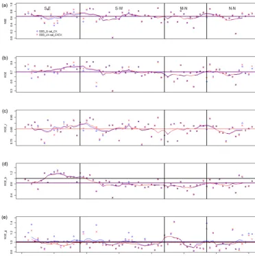
given by the ratio of the coefficients of variation of simulated and observed runoff as suggested in Kling et al. (2012). The mean values of the skill scores for DDD_LN and DDD_G are shown in Table 2 and as straight lines in the plots. We have also added a moving average of the results for enhanced read-ability. We see from the Fig. 5 and Table 2 that little precision in predicting runoff is lost when using DDD_G. The mean values for NSE, KGE and the different elements of KGE are practically identical. Differences between runoff simu-lations for DDD_G and DDD_LN are mostly pronounced in the south-east, where, especially for NSE, DDD_LN appears to be consistently better.
Table 3 shows that significant correlation between NSE and CC was only found for catchment area. Such a correla-tion was not found for KGE; rather, significant negative cor-relation were found for both models between KGE and the areal fraction of bare rock.
Table 2.Mean values of skill scores for the validation period 2000– 2014 simulated with DDD_G and DDD_LN for 71 catchments. KGE_r measures correlation, KGE_b, the bias error and KGE_g the variability error. All skill scores have an ideal value of 1.
NSE KGE KGE_r KGE_b KGE_g
DDD_G 0.64 0.70 0.85 0.85 1.02 DDD_LN 0.65 0.71 0.85 0.84 0.99
3.2 Snow water equivalent
Figure 5.Skill scores for DDD_G (blue circles) and DDD_LN (red crosses) for 71 Norwegian catchments. Mean skill score values are shown in horizontal lines along with moving averages (same colour code).(a)NSE,(b)KGE,(c)KGE_r (correlation),(d)KGE_b (bias) and(e)KGE_g (variability error). The results are organized into the regions south-east (S-E), south-west (S-W), mid-Norway (M-N) and Northern Norway (N-N) as indicated in Fig. 3.
Table 3.Spearman correlations between simulated model results and catchment characteristics for the validation period 2000–2014. Only significant correlations are shown (p value < 0.01) except for the correlation marked ∗, which has a p value slightly larger than 0.01 (pvalue=0.013).
Catchment size Lake (%) Bog (%) Bare rock (%) Forest (%) Mean elevation
NSE DDD_G 0.38
DDD_LN 0.38
KGE DDD_G −0.33
DDD_LN −0.35
Slope SWE DDD_G 0.38 −0.46 0.44 −0.40
SCA_RMSE DDD_G −0.3∗
DDD_LN −0.34
SCA_MAE DDD_G 0.50 −0.40 DDD_LN 0.44 −0.42
Duration of snow cover DDD_G 0.32 0.67 −0.63 0.73
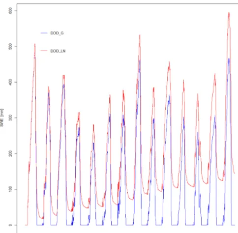
Figure 6.Time series of simulated SWE using DDD_G (blue line) and DDD_LN (red line) for catchment Tansvatn in Southern Nor-way.
deviates increasingly as time proceeds. Figure 7a shows a scatter plot of the mean simulated SWE (averaged over the time series) for the 71 catchments by the two models and it is clearly seen that SWE simulated by DDD_LN is higher than simulated by DDD_G although both the precipitation and temperature input are identical for the two models. From linear regression between SWE, precipitation and tempera-ture with time we can estimate simple annual trends. Fig-ure 7b, c, d show plots of the slopes of the regression lines. Whereas both precipitation and temperature show very mod-est annual rates of change, both models simulate increasing SWE with time, but DDD_LN, on average, 5 times as much as DDD_G. If 100 days a year may serve as an estimate of days with solid precipitation, the increase in SWE due to the positive trend in precipitation comes very close to the trend in SWE found for DDD_G. Positive trends of SWE greater than 5 mm year−1was found for 26 out of 71 (37 %) catchments for DDD_LN model and 7 out of 71 catchments (10 %) for the DDD_G model.
The regression slopes of SWE for both models were cor-related with CC and for DDD_LN no significant correlations were found. Significant correlation was, however, found be-tween the slopes of SWE for DDD_LN and the parameter values ofθCV,rS_SWE,θCV=0.45, which in turn is signifi-cantly correlated with skill score KGE,rKGE_LN, θCV=0.40. For DDD_G significant correlations were found between the slopes and lakes, bare rock, bogs and forest.
3.3 Snow-covered area and snow cover duration
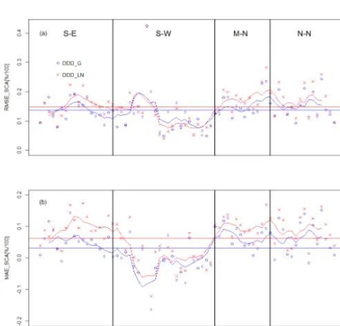
Figure 8a shows the root mean square error (RMSE) between observed and simulated catchment values of SCA for 69 catchments. Although the mean RMSE does not differ much between the two models (mean(RMSE)=0.14 for DDD_G and mean(RMSE)=0.15 for DDD_LN) we can note that SCA is better estimated using DDD_G for 46 out of 69 catch-ments (67 %). DDD_LN appears to be better in the south-western part of Norway whereas DDD_G performs better in the other regions. The mean elevation of catchments was found to be significantly correlated to RMSE for simulated SCA using DDD_LN and nearly significantly correlated us-ing DDD_G. The correlation implies that the errors in esti-mating SCA are, for both models, reduced as the mean ele-vation of the catchments increase. Figure 8b shows the mean absolute error (MAE) and we see that DDD_G is the supe-rior method with respect to MAE for all regions except for the south-west. The errors are mostly positive indicating a general overestimation of SCA, although underestimation is also found in south-western Norway. The mean value over all the catchments is mean(MAE)=0.03 for DDD_G and mean(MAE)=0.06 for DDD_LN. For both models, MAE was significantly correlated to the areal percentage of lakes and the size of the catchment, but not the mean elevation.
The mean annual snow cover duration was calculated as the mean number of days with snow present in the catchment and is shown in Fig. 9. There is a striking difference in this results between DDD_LN and DDD_G. The mean duration of the snow cover of DDD_LN shows almost no variability, is very high and suggests an almost perennial snow cover. This result is consistent with the positive trends for SWE as-sociated with DDD_LN. From Table 3 we see that the snow cover duration are, for both models, significantly correlated with catchment size, fraction of forest and bare rock and the mean elevation of the catchment.
4 Discussion
Figure 7.Scatter plots of mean SWE simulated with DDD_G and DDD_LN for 71 catchments(a), annual slope of SWE(b), annual slope of precipitation(c)and temperature(d).
Figure 8. (a)Root mean square error (RMSE) for simulated SCA for DDD_G (blue) and DDD_LN (red). (b) Mean absolute error (MAE) for simulated SCA for DDD_G (blue) and DDD_LN (red). Moving averages and mean values of RMSE and MAE are shown with the same colour code.
to properly assess the hydrological effects of climate change and to provide useful predictions for ungauged basins, we have to move towards the use of hydrological models with a minimum of calibration parameters.
Figure 9. Mean annual days of snowcover in the catchments for DDD_LN (red) and DDD_G (blue). Moving averages are shown using the same colour code.
a log-normal distribution for SWE with a fixed, calibrated CV has recently been addressed in the literature (Frey and Holzmann, 2015). In Norway, using such a snow distribution model with the well-known Swedish rainfall–runoff model, HBV (Hydrologiska Byråns Vattenbalansmodell; Bergström, 1992), has led to the operational procedure of deleting the remaining snow reservoir at the end of summer. Such a pro-cedure clearly constitutes an example of a model working well (with respect to runoff) but not for the right reasons. This point is further illustrated when we focus on one of the catchments that gives better NSE values using DDD_LN than DDD_G.
The Masi catchment (5543 km2) is located in Northern Norway and is relatively flat (90 % of its area is located below 600 m a.s.l. and its minimum and maximum elevation is 370 and 1085 m a.s.l. respectively) so that the snow melt season is quite short and intense. Figure 10a shows the simulation of SWE using SD_LN with optimized CV (θCV=0.88), which gave a NSE value for runoff of NSE=0.75, and using SD_G, which gave a NSE value for runoff equal to NSE=0.72. In Fig. 10b we have adjusted the CV value from θCV=0.88 to θCV=0.1, and the simulation of SWE using SD_LN no longer exhibits the very strong positive trend seen in Fig. 10a; it looks more realistic and very similar to that of SD_G. The precision of runoff simulation was, however, affected and the NSE value dropped from NSE=0.75 to NSE=0.60. A rea-sonable conclusion may thus be that the slightly higher val-ues for NSE and KGE using SD_LN is at the expense of unrealistic values of SWE. The correlation analysis supports this conclusion (see Table 3). The increase in SWE with time
Figure 10. Time series of simulated SWE for the Masi catch-ment in Northern Norway with DDD_G (blue) and DDD_LN (red). In(a)SWE is simulated with optimized CV=0.77, which gives a NSE=0.75. In (b) SWE is simulated with adjusted CV=0.1, which gives a NSE=0.60. Using DDD_G gives a NSE=0.72.
of DDD_LN is not correlated to any CC but to the parameter values of the method for spatial distribution of SWE,θCV. The parameterθCVis found to be significantly correlated to the skill score for predicting runoff, KGE; i.e. high values ofθCVgives high values of KGE. The high skill scores for DDD_LN are clearly not due to a realistic process descrip-tion of snow but rather to an inadequate model structure that gets it right for the wrong reasons.
dif-Figure 11.Time series of simulated SCA with DDD_G (blue) and DDD_LN (red) together with MODIS derived SCA (green circles) for catchment Tansvatn in Southern Norway.
ficult. DDD_G, in contrast, provides an accumulation dis-tribution without the heavy tail, which appears as a better choice with respect to the simulation of both SWE and SCA. The difference between the two methods with respect to the modelling of SCA became very clear when we compared the average annual duration of the snow cover. DDD_ LN, due to the positive trends in SWE, ended up with an almost perennial snow cover for most of the catchments (see Fig. 9), whereas DDD_G showed a variability in snow cover dura-tions that is more consistent with the varying climate in Nor-way. For both models the correlation analysis between snow cover duration and CC showed that the duration of snow cover was positively correlated to catchment size, mean ele-vation and areal fraction of bare rock (area above the treeline) and negatively correlated to the areal fraction of forest. Since the areal fraction of forest and bare rock is highly correlated, these are expected relations illustrating that both models have a realistic snow distribution with respect to elevation.
A more realistically simulated SCA is important for many applications. Updating of snow and hydrological models us-ing observed SCA is dependent on realistic simulations of SCA. A realistic simulation of SCA is also necessary for the properly accounting of energy fluxes over an area partly covered by snow (Liston, 1999; Essery and Pomeroy, 2004) and is hence important for the assessment of hydrological impacts of climate change. Without realistically simulated SCA, we cannot expect credible simulations for climate pro-jections for neither runoff dynamics nor energy fluxes.
SWE is represented here as the sum of correlated (in time) spatial variables (solid precipitation). Precipitation events such as snow are assumed to be gamma distributed in space
with parameters varying with intensity. The parameter scale,
α0, and decorrelation length,D, are estimated from observed spatial moments of precipitation. Recall that the shape pa-rameterν0, is just set as one-tenth ofα0through the relation
E (y)=ν0
α0
=0.1 mm. From Fig. 1 we see that the variance levels off, and even decreases, for increased spatial mean in-tensity. The presented model captures this observed feature since the variance will cease to increase as the correlation de-creases with intensity (the number of summations). As cor-relation approaches 0, we will have a sum of independent events. According to the central limit theorem, such a sum will have a normal distribution. The shape parameter ofy,
ν0and the correlation determines the rate of the convergence to a normal distribution. For example, if the decorrelation range is long, then more summations are needed for the spa-tial frequency distribution of SWE to approach a normal dis-tribution. The literature shows that empirical spatial distribu-tion of SWE has a tendency to be positively skewed. This is especially the case for many observations of SWE in Nor-way in high alpine areas (Alfnes et al., 2004; Marchand and Killingtveit, 2004; Marchand and Killingtveit, 2005). For more lowland and forested areas, the distribution tends to be more normal (Alfnes et al, 2004; Marchand and Killingtveit, 2004; Marchand and Killingtveit, 2005). In our modelling framework, this would imply that we would expect small shape parameters and long decorrelation lengths for moun-tain areas and larger shape parameters together with short decorrelation lengths for lower-lying forested areas. Table 4 show correlations and their significance (pvalues) between the parametersα0andDand the CC fraction of bare rock, fraction of forest, mean elevation and catchment area. We see thatα0is significantly correlated to the mountain/forest and highland/lowland indices as expected. The decorrelation length D is weakly correlated to the mean elevation in a way implying shorter correlation lengths at high altitudes, i.e. contrary to what is expected from reported shapes of the PDF of SWE, and uncorrelated to the other indices. It is promising, and somewhat unexpected, that correlation be-tweenα0(ν0)and catchment characteristics supports our the-ory so clearly since the location of Norwegian precipitation gauges, which is has a very poor representation at high ele-vations (Dyrrdal et al., 2012; Saloranta, 2012), was not ex-pected to discriminate this behaviour very well. The some-what confusing results of the decorrelation length suggest a dedicated study using a more dense network of precipitation gauges.
Table 4. Spearman correlations between model parameters and catchment characteristics indicating alpine and lowland areas where the spatial distribution of SWE is expected to vary. The bracketed numbers indicate significance (pvalue).
Forest (%) Bare rock (%) Mean elevation Catchment size
α0 0.34 (0.00) −0.40 (0.00) −0.35 (0.00) −0.28 (0.02)
D 0.13 (0.29) −0.14 (0.24) −0.25 (0.03) −0.15 (0.19)
2011; Mott et al., 2011; Scipion et al., 2013) and, in addi-tion, various spatial scales and landscape types interact and further complicate the matter (Blöschl, 1999; Alfnes et al. 2004; Liston, 2004; Marchand and Killingtveit, 2004; Marc-hand and Killingtveit, 2005). A major problem is that the spatial distribution of snow and SWE is very hard to mea-sure at the appropriate scale, i.e. the catchment scale, which often covers different elevations and both forested and open (alpine) areas. Various airborne observation techniques such as laser scan (Melvold and Skaugen, 2013) and passive mi-crowave (Vuyovich, 2014) are promising but restricted by landscape features such as vegetation and topography and the state of the snow (wet/dry). Consequently, investigations on the spatial distribution of SWE has to rely on in situ mea-surements, which seldom covers entire catchments. In this study, in situ information (the spatial variability of solid and liquid precipitation), is obtained from the station network of precipitation gauges of the Norwegian Meteorological Insti-tute, which measures precipitation at 2 m above ground. It is highly probable that the observed spatial variability, mea-sured near to the surface, captures information of the influ-ence of the wind on precipitation in general and on snow-fall in particular. This assumption is justified by the signif-icant and relatively high correlations seen in Table 4 be-tween the scale parameter, α0 (and hence, in our case, the shape parameter,ν0), and landscape features such as eleva-tion and vegetaeleva-tion and suggests a sensitivity to the exposure of wind. Johansson and Chen (2003) demonstrate the influ-ence of wind speed on the spatial distribution of precipitation and Mott et al. (2011) and Lehning et al. (2008) show that near-surface wind fields highly influence snow distribution patterns through preferential deposition.
The method presented in this study does not include re-distribution of SWE due to wind as a driving force for shap-ing the spatial frequency distribution of SWE at the catch-ment scale. Some authors suggest that this process occurs on a spatial scale much smaller than the catchment scale (Lis-ton, 2004; Melvold and Skaugen, 2013). In Figure 11 we see that DDD_LN shows a better simulation of SCA for the start of the melting period than DDD_G for at least two of the years (2011 and 2014). The reason to why DDD_LN simu-lates the initial development of snow-free areas better than DDD_G is probably that SD_LN produces a generally more positively skewed distribution of SWE than SD_G, and has, hence, a higher frequency of small values of SWE that melts
quickly. Whereas the distribution of SD_G, which in general seems to be more appropriate, should perhaps have a frac-tion of the catchment populated with small values of SWE in order to simulate this observed initial development of snow-free areas. By including redistribution due to wind, we might produce areas of shallow SWE, such as over wind-exposed ridges which are known to become free of snow rather early in spring.
Finally, it is important to keep in mind that this study aims at determining the spatial frequency distribution of SWE for elevation bands for a catchment. These areas may comprise several square kilometres. The spatial distribution of SWE for distributed hydrological modelling, i.e. simulating the amount of SWE at specific locations, is another, much more challenging, task which involves taking into account very small-scale (< 25 m according to Lehning et al., 2008) land-scape features and their complex relation to accumulation, melting and redistribution of SWE.
5 Conclusions
In this paper a method for estimating the spatial frequency distribution of SWE is implemented in the parameter parsi-monious rainfall–runoff model DDD. The new method, first described by Skaugen (2007) and further developed by Skau-gen and Randen (2013) and here, has its parameters esti-mated from observed spatial variability of precipitation mea-sured from precipitation gauges. The new method (SD_G) has hence no parameters to be optimized from calibration against runoff unlike the current operational snow distribu-tion routine (SD_LN), which has one calibradistribu-tion parameter. The new method gives a dynamic presentation of the distri-bution of SWE, which, at the start of the accumulation sea-son, may be positively skewed but converges to a more sym-metrical distribution as the accumulation season progresses. The parameters of the method show significant correlations with catchment characteristics discriminating between shel-tered and wind-exposed areas.
MODIS-derived SCA and SD_G has the lower RMSE. The differ-ence in simulated SCA between the two models is especially seen for median to low values of SCA. SD_LN can be seen to simulate better SCA at the beginning of the melt season, suggesting that SD_G has a too-low frequency of low SWE values.
6 Data availability
NVE supports an open data policy; real-time and near-real-time data are available at http://www.nve.no/en/15Water/ Data-databaser/Real-time-hydrological-data/ and historical data are freely available at request to [email protected].
Acknowledgements. The help of Nils Kristian Orthe at NVE in providing the satellite-derived SCA data is gratefully acknowl-edged. This work was partly conducted in the project “Better SNOW models for natural hazards and HydropOWer applications” (SNOWHOW) (project 244153) funded by the Norwegian Re-search Council.
Edited by: R. Brown
Reviewed by: two anonymous referees
References
Alfnes, E., Andreassen, L. M, Engeset, R. V., Skaugen, T., and Udnæs, H-C.: Temporal variability in snow distribution, Ann. Glaciol., 38, 101–105, 2004.
Anderson, E. A.: A point Energy and Mass Balance model of a snow cover, NOAA Technical Report NWS 19, US Dept. of Com-merce, Silver Spring, MD, 150 pp., 1976.
Bergström, S.: The HBV model – its structure and applications, SMHI Reports Hydrology No. 4, Swedish Meteorological and Hydrological Institute, Norrköping, Sweden, 32 pp., 1992. Blöschl, G.: Scaling issues in snow hydrology, Hydrol. Process., 13,
2149–2175, 1999.
Buttle, J. M. and McDonnel, J. J.: Modelling the areal depletion of snowcover in a forested catchment, J. Hydrol., 90, 43–60, 1987. Clark, M. P., Hendrix, J., Slater, A. G., Kavetski, D., Anderson, B., Cullen, N. J., Kerr, T., Hreinsson, E. Ö., and Woods, R. A.: Rep-resenting spatial variability of snow water equivalent in hydro-logical and land- surface models: A review, Water Resour. Res., 47, W07539, doi:10.1029/2011WR010745, 2011.
Dingman, S. L.: Physical hydrology, edited by: Lynch, P., Prentice Hall, New Jersey, USA, 646 pp., 2002.
Donald, J. R., Soulis, E. D., Kouwen, N., and Pietroniro, A.: A land cover-based snow cover representation for distributed hydrologic models, Water Resour. Res., 31, 995–1009, 1995.
Dyrrdal A. V., Saloranta, T., Skaugen, T., and Stranden, H.-B.: Changes in snow depth in Norway during the period 1961–2010, Hydrol. Res., 44, 169–179, doi:10.2166/nh.2012.064, 2013. Essery, R. and Pomeroy, J.: Implications of spatial distributions of
snow mass and melt rate for snow-cover depletion: theoretical considerations. Ann. Glaciol., 38, 261–265, 2004.
Frey, S. and Holzmann, H.: A conceptual, distributed snow re-distribution model, Hydrol. Earth Syst. Sci., 19, 4517–4530, doi:10.5194/hess-19-4517-2015, 2015.
Gupta, H. V., Kling, H., Yilmaz, K. K., and Martinez, G. F.: Decom-position of the mean squared error and NSE performance criteria: implications for improving hydrological modelling, J. Hydrol., 377, 80–91, doi:10.1016/j.jhydrol.2009.08.003, 2009.
Haan, C. T.: Statistical methods in hydrology, The Iowa State Uni-versity Press, Ames, Iowa, 378 pp., 1977.
Helbig, N., van Herwijnen, A., Magnusson, J., and Jonas, T.: Fractional snow-covered area parameterization over com-plex topography, Hydrol. Earth Syst. Sci., 19, 1339–1351, doi:10.5194/hess-19-1339-2015, 2015.
Hock, R.: Glacier melt: a review of processes and their modelling, Prog. Phys. Geog., 29, 362–391, 2005.
Johansson, B. and Cheng, D.:The influence of wind and topography on precipitation distribution in Sweden: Statistical analysis and modelling, Int. J. Climatol., 23, 1523–1535, doi:10.1002/joc.951, 2003.
Killingtveit, Å. and Sælthun, N-R.: Hydrology, (Volume No. 7 in Hydropower development), Norwegian Institute of Technology – NIT, Trondheim, Norway, 213 pp., 1995.
Kirchner J. W.: Getting the right answers for the right rea-sons: Linking measurements, analyses and models to advance the science of hydrology, Water Resour. Res., 42, W03S04, doi:10.1029/2005WR004362, 2006.
Kling, H., Fuchs, M., and Paulin, M.: Runoff conditions in the up-per danube basin under an ensemble of climate change scenarios, J. Hydrol., 424, 264–277, doi:10.1016/j.jhydrol.2012.01.011, 2012.
Kolberg, S. and Gottschalk, L.: Interannual stability of grid cell snow depletion curves as estimated from MODIS images, Water Resour. Res., 46, W11555, doi:10.1029/2008WR007617, 2010. Kutchment, L. S. and Gelfan, A. N.: The determination of the
snowmelt rate and the meltwater outflow from a snowpack for modelling river runoff generation, J. Hydrol., 179, 23–36, 1996. Lehning, M., Löwe, H., Ryser, M., and Raderschall, N.: Inhomogeneous precipitation distribution and snow trans-port in steep terrain, Water Resour. Res., 44, W07404, doi:10.1029/2007WR006545, 2008.
Liston, G.: Interrelationships among Snow Distribution, Snowmelt and Snow Cover Depletion: implications for atmospheric, hydro-logic and ecohydro-logic modeling, J. App. Meteor., 38, 1474–1487, 1999.
Liston, G. E.: Representing subgrid snow cover heterogeneities in regional and global models, J. Climate, 17, 1381–1397, 2004. Luce, C. H., Tarboton, D. G., and Cooley, K. R.: Sub-grid
param-eterization of snow distribution for an energy and mass balance snow cover model, Hydrol. Process., 13, 1921–1933, 1999. Luce, C. H. and Tarboton, D. G: The application of depletion curves
for parameterization of subgrid variability of snow, Hydrol. Pro-cess., 18, 1409–1422, 2004.
Lussana, C. and Tveito, O.-E.: Spatial Interpolation of precipitation using Bayesian methods, Unpublished research note, The Nor-wegian Meteorological Institute, Oslo, Norway, 2014a. Lussana, C. and Tveito, O.-E.: Spatial Interpolation of temperature
Marchand, W.-D. and Killingtveit, Å.: Statistical properties of spa-tial snowcover in mountainous catchments in Norway, Nordic Hydrol., 35, 101–117, 2004.
Marchand, W.-D. and Killingtveit, Å.: Statistical probability dis-tribution of snow depth at the model sub-grid cell spatial scale, Hydrol. Process., 19, 355–369, 2005.
Melvold, K. and Skaugen, T.: Multiscale spatial variability of lidar-derived and modeled snow depth on Hardangervidda, Nor-way, Ann. Glaciol., 54, 273–281, doi:10.3189/2013AoG62A161, 2013.
Mott, R., Schirmer, M., and Lehning, M.: Scaling properties and snow depth distribution in an alpine catchment, J. Geophys. Res., 116, D06106, doi:10.1029/2010JD014886, 2011.
Nash, J. E. and Sutcliffe, J. V.: River flow forecasting through con-ceptual models, Part 1 – a discussion of principles, J. Hydrol., 10, 282–290, 1970.
Omhura, A.: Physical basis for the temperature-based melt-index method, J. Appl. Meteorol., 40, 753–761, 2001.
Parajka, J., Merz, R., and Blöschl, G.: Uncertainty and multiple ob-jective calibration in regional water balance modelling: a case study in 320 Austrian catchments, Hydrol. Process., 21, 435– 446, 2007.
Salomonson, V. V. and Apple, I.: Estimating fractional snow cover from MODIS using the normalized difference snow index, Re-mote Sens. Environ., 89, 351–361, 2004.
Saloranta, T. M.: Simulating snow maps for Norway: descrip-tion and statistical evaluadescrip-tion of the seNorge snow model, The Cryosphere, 6, 1323–1337, doi:10.5194/tc-6-1323-2012, 2012. Scipion, D. E., Mott, R., Lehning, M., Schneebeli, M., and Berne,
A.: Seasonal small-scale spatial variability in alpine snowfall and snow accumulation, Water Resour. Res., 49, 1446–1457, doi:10.1002/Wrcr.20135, 2013.
Skaugen, T.: Modelling the spatial variability of snow water equiv-alent at the catchment scale, Hydrol. Earth Syst. Sci., 11, 1543– 1550, doi:10.5194/hess-11-1543-2007, 2007.
Skaugen, T. and Andersen, J.: Simulated precipitation fields with variance-consistent Interpolation, Hydrolog. Sci. J., 55, 676–686, doi:10.1080/02626667.2010.487976, 2010.
Skaugen T. and Onof, C.: A rainfall runoff model parameterized form GIS and runoff data, Hydrol. Process., 28, 4529–4542, doi:10.1002/hyp.9968, 2014.
Skaugen, T., Peerebom, I. O., and Nilsson, A.: Use of a parsi-monious rainfall-runoff model for predicting hydrological re-sponse in ungauged basins, Hydrol. Process., 29, 1999–2013, doi:10.1002/hyp.10315, 2015.
Skaugen, T. and Mengistu, Z.: Estimating catchment scale ground-water dynamics from recession analysis – enhanced constraining of hydrological models, Hydrol. Earth Syst. Sci. Discuss., 12, 11129–11171, doi:10.5194/hessd-12-11129-2015, 2015. Skaugen, T. and Randen, F.: Modeling the spatial
distri-bution of snow water equivalent, taking into account changes in snow-covered area, Ann. Glaciol., 54, 180–186, doi:10.3189/2013AoG62A162, 2013.
Soetart, K. and Petzholdt, T.: Inverse modelling, sensitivity and Monte Carlo analysis in R using package FME, J. Stat. Softw., 33, 1–28, www.jstatsoft.org/article/view/v033i03/ v33i03.pdf (last access: 29 October 2015), 2010.
Solberg, R., Koren, H., and Amlien, J.: A review of optical snow cover algorithms, SAMBA/40/06, Norwegian Computing Cen-tre, Norway, 15 December, 2006.
Sælthun, N. R.: The “Nordic” HBV model. Description and docu-mentation of the model version developed for the project Climate Change and Energy Production, NVE Publication no. 7-1996, Oslo, 26 pp., 1996.
Vuyovich, C. M., Jacobs, J. M., and Daly, S. F.: Comparison of pas-sive microwave and modeled estimates of total watershed SWE in continental United States, Water Resour. Res., 50, 9088–9102, doi:10.1002/2013WR014734, 2014.
Weltzien, I. H.: Parsimonious snow modelling for application in hydrological models. Ms.Sci. thesis, University of Oslo, Nor-way, available at: https://www.duo.uio.no/handle/10852/46121 (last access: 2 September 2016), 2015.
Zawadski, , I. I.: Statistical properties of precipitation patterns, J. Appl. Meteorol., 12, 459–472, 1973.