MODELING AND FORECASTING DAILY STOCK RETURNS OF GUARANTY TRUST BANK NIGERIA PLC USING ARMA-GARCH MODELS, PERSISTENCE, HALF-LIFE VOLATILITY AND BACKTESTING

(1)

Published by Faculty of Science, Kaduna State University

Modeling and forecasting Daily stock Returns of Guaranty Trust Bank Nigeria Plc

Using ARMA-GARCH Models, Persistence, Half-life Volatility and Backtesting

MODELING AND FORECASTING DAILY STOCK RETURNS OF

GUARANTY TRUST BANK NIGERIA PLC USING ARMA-GARCH

MODELS, PERSISTENCE, HALF-LIFE VOLATILITY AND

BACKTESTING

Ngozi G. Emenogu1*_{; Monday Osagie Adenomon}2,4*_{and Nweze Obinna Nwaze}3

1_{Department of Statistics, Federal Polytechnic, Bida, Niger State, Nigeria}

2,3_{Department of Statistics & NSUK-LISA Stat Lab, Nasarawa State University, Keffi, Nasarawa State, Nigeria} 4_{Foundation of Laboratory Econometrics and Applied Statistics of Nigeria (aka FOUND-LEAS-IN-NIGERIA)}

*Corresponding Author Email Address:[email protected] Phone: +2347036990145 ABSTRACT

This study investigated the forecasting ability of GARCH family models, and to achieve superior and more reliable models for volatility persistence, half-life volatility and backtesting, the study combined the ARMA and GARCH models. The study modeled and forecasted the Guaranty Trust Bank (GTB) daily stock returns using data from January 2, 2001 to May 8, 2017 obtained from a secondary source. The ARMA-GARCH models, persistence, half-life and backtesting were used to analyse the data using student t and skewed student t distributions, and the analyses were carried out in R environment using rugarch and performanceAnaytics Packages. The study revealed that using the lowest information criteria values alone could be misleading so backtesing was also carried out. The ARMA(1,1)-GARCH(1,1) models fitted exhibited high persistency in the daily stock returns while it took about 6 days for mean-reverting of the models, but failed backtesting. However, backtesting showed that ARMA(1,1)-eGARCH(2,2) model with student t distribution passed the test and was suitable for evaluating the GTB stock returns, and required about 16 days for the persistence volatility to return to its average value of the stock returns. The study recommended addition of backtesting approach in evaluating the performance of GARCH model in order to avoid misleading results. Also, the GTB stocks can be predicted since most of the estimated models were stable.

Keywords: Stock returns, Guaranty Trust (GT) Bank, Generalized Autoregressive Conditional Heteroskedasticity (GARCH), Persistence, Volatility, Backtesting

INTRODUCTION

Autoregressive Moving Average (ARMA) and Autoregressive Integrated Moving Average (ARIMA) models are popular and excellent for modeling and forecasting univariate time series data as proposed by Box & Jenkins (1970), and its extension with exogenous variables as Autoregressive Integrated Moving Average with Explanatory Variable (ARIMAX) (Kongcharoen & Kruangpradit, 2013). These models are applied in almost all fields of endeavours such as engineering, geophysics, business, economics, finance, agriculture, medical sciences, social sciences, meteorology, quality control etc. (Kirchgassner & Wolters, 2007; Adenomon, 2017a; Adenomon, 2017b; Cooray, 2008; Dobre & Alexandru, 2008; Gujarati, 2003; Adekeye & Aiyelabegan, 2006). The ARMA and ARIMA models are used to

model conditional expectation of a process but in ARMA model, the conditional variance is constant. This means that ARMA model cannot capture process with time-varying conditional variance (volatility) which is mostly common with economic and financial time series data.

Actually, with economic and financial time series data, time-varying is more common than constant volatility, and accurate modeling of time volatility is of great importance in financial time series analysis (Ruppert, 2011). Financial time series contains uncertainty, volatility, excess kurtosis, high standard deviation, high skewness and sometimes non normality (Pedroni, 2001; Grigoletto & Lisi, 2009; Emenogu & Adenomon, 2018; Emenogu

et al., 2018). To model and capture properly the characteristics of financial time series models such as Auto-Regressive Conditional Heteroscedastic (ARCH), Generalized Auto-Regressive Conditional Heteroscedastic (GARCH), multivariate GARCH, Stochastic volatitlity (SV) and various variants of the models have been proposed to handle these characteristics of financial time series (Lawrance, 2013).

From the foregoing, considering the flexibility and simplicity of the ARMA model and the capability of the GARCH model to capture volatility in financial time series, combining the ARMA model with the GARCH model for the innovations, yielding the so-called ARMA-GARCH model, provides the econometricians and financial analyst with a more flexible and yet tractable model that allows the model to capture the mean and variance components that is common with financial time series volatility (Lange, 2011; Panait & Slavescu, 2012) meaning that the ARMA-GARCH model will produced more reliable estimates for financial analyst to take a better decision. Most financial time series analyses in Nigeria scarcely incorporate backtesting approach in selecting GARCH models.

This paper therefore investigates the persistence, half-life volatility and forecasting (Backtesting that is providing real life model) of daily stock returns of Guaranty Trust Bank, Nigeria plc using ARMA-GARCH Models. The remaining sections are as follows: Empirical review, Materials and Methods, Results, Discussion of Results, Conclusion and Recommendations.

Fu

ll L

en

gt

h Rese

ar

ch

(2)

Modeling and forecasting Daily stock Returns of Guaranty Trust Bank Nigeria Plc

Empirical literature on the persistence, half-life Volatility and

Backtesting of Stocks Returns

The volatility of asset returns is a measure of how much the returns fluctuates around its means (Marra, 2015). In addition, volatility is the purest measure of risk in financial markets and by this, it has becomes the expected price of uncertainty. A good volatility model and forecast help impact the public confidence significantly and by extension on the broader global economy. What comes to mind again is the persistence and half-life volatility of any given stock.

The persistence of financial stock is the extent to which events today have an efficient influence on the whole future history of a stochastic process, and as such is a central issue in financial time series, macroeconomic theory and policy (Caporale & Pittis, 2001). In a stationary GARCH process, the persistence volatility returns back to its means at the long term horizon and it is a rate calculated by the sum of GARCH and ARCH coefficients. And in many financial time series it is usually close to 1 (Ahmed et al., 2018; Engle & Patton, 2001; Vosvrda, 2006). While on the other hand, the half-life of the volatility shocks measure the average time period for the volatility to return back to it mean value in the long run horizon (Ahmed et al., 2018; Sahai, 2016).

Engle & Patton (2001) examined the Dow Jones Industrial index from 23 August 1988 to 22 August 2000. Their result indicated that the volatility returns are quite persistent.

Magnus & Fosu (2006) modeled and forecasted the volatility of returns on Ghana Stock exchange using GARCH models. They found that presence of high level of persistence in the returns in the stock market.

Vosvrda (2006) compared empirical analysis of persistence and dependence patterns among capital market using univariate and multivariate measures. The results revealed that the univariate measure shows a low level of persistence while multivariate measure shows that the persistence change depended on structure in different period of lags.

Panait & Slavescus (2012) investigated the volatility and persistence of seven Romanian companies traded on Bucharest Stock Exchange and three market indices from 1997-2012 using GARCH-in-Mean Models. They found out that persistency is more in the daily returns as compared to weekly and monthly series.

Emenike & Ani (2014) examined the nature of volatility of stock returns in the Nigerian banking sector using ARMA-GARCH models using data covering 3rd_{January to December 2012. Their} results revealed volatility persistence was high for the sample period they considered.

Usman et al. (2017) examined the performance of eleven competing GARCH models for fitting the rate of returns of monthly observations on the index returns series of the market over a period of January 1996 to December 2015. The overall results revealed increased volatility of the market returns.

Chu et al. (2017) provided the first GARCH modeling of the seven most popular cryptocurrencies using twelve GARCH models fitted for each cryptocurrencies. Their work concluded IGARCH and

GJR-GARCH models provided the best fits in terms of modeling of the volatility in the most popular and largest cryptocurrencies.

Kuhe (2018) examined the volatility persistence and asymmetry with exogenous break in Nigerian stock market using data from 3rd_{July 1999 to 12}th_{June 2017 using standard symmetric} GARCH (1,1), asymmetric EGARCH (1,1) and GJR-GARCH (1,1) models. The study revealed among other results a high persistence of shocks in the return series for the estimated models.

Ahmed et al. (2018) examined and compared the mean reversion phenomenon in developed and emerging stock markets, it employed data from 1st_{January to 30}th_{June 2016 using GARCH} (1,1) model. There results revealed that South Korean market has the slowest mean reversion and thus has the highest half-life period while Pakistan stock exhibited fastest reverting process.

Backtesting approach is very useful in GARCH model selection, but not often applied in the Nigerian context. Summinga-Sonagadu and Narsoo (2019) employed three backtesting procudures namely Kupiec’s test, a duration-based test and an asymmetric VaR loss function on Intraday of 1-min EUR/USD exchange rate returns. Their results revealed that VaR prediction of the MC-GARCH model performed better using the asymmetric loss function.

Tay et al. (2019) investigated the efficiency of the Value-at-Risk (VaR) backtesting in model selection from different types of GARCH models with skewed and non-skewed innovation distributions. The study implemented both simulation and real life data application (NASDAQ Index). The study revealed that AIC and VaR backtesting approach were able to select the correct model with their corresponding innovation distributions.

MATERIALS AND METHODS

Model Specification

ARMA-GARCH Models

This study focuses on the ARMA-GARCH models that are robust for forecasting the volatility of financial time series data; so ARMA-GARCH model and some of its extensions are presented in this section.

ARMA-GARCH specification is employed to model the conditional mean and conditional variance (volatility) of any financial time series because of its superiority in modelling such series. GARCH models model conditional variances much as the conditional expectation by an ARMA model (Ruppert 2011). Therefore ARMA model can be combined to any form of GARCH model.

The ARMA (p,q)-GARCH (1,1) model can be specified as follows: ARMA(p,q)-GARCH(1,1) model can be specified as follows:

𝑟𝑡= ∑𝑝𝑖=1𝜃𝑖𝑟𝑡−𝑖+ ∑𝑞𝑗=1𝜙𝑗𝜖𝑡−𝑗+ 𝜖𝑡

𝜖𝑡√𝜎𝑡2𝑍𝑡 , 𝑍𝑡~ 𝐷(0, 𝜎𝑡2)

𝜎𝑡2= 𝜔 + 𝛼1𝜖𝑡−12 + 𝛽1𝜎𝑡−12

} (1)

(3)

Modeling and forecasting Daily stock Returns of Guaranty Trust Bank Nigeria Plc

Where, 𝑟𝑡 is the daily rate of return, 𝜃 is the AR(p) term in the

mean equation in order to account for time dependence in returns, 𝜙 is the MA(q) term in the mean equation, 𝜖𝑡 is the

residual term in the mean equation, 𝑍𝑡 is the standardized

residual sequence of 𝑖𝑖𝑑 random variable with mean zero and variance 𝜎𝑡2, while 𝐷 represents distribution of the shock returns.

TGARCH(p, q) Model

The Threshold GARCH model is another model used to handle leverage effects, and a TGARCH (p, q) model is given by the following:

𝜎𝑡2= 𝛼0+ ∑ (𝛼𝑖+ 𝛾𝑖𝑁𝑡−𝑖)2𝑎𝑡−𝑖2 + ∑𝑞𝑗=1𝛽𝑗𝜎𝑡−𝑗2 𝑝

𝑖=1 (2)

where 𝑁𝑡−𝑖is an indicator for negative 𝑎𝑡−𝑖, that is,

𝑁𝑡−𝑖= {

1 𝑖𝑓 𝜖𝑡−𝑖< 0,

0 𝑖𝑓 𝜖𝑡−𝑖≥ 0,

and 𝛼𝑖, 𝛾𝑖 and 𝛽𝑗 are nonnegative parameters satisfying

conditions similar to those of GARCH models, (Tsay, 2005). When 𝑝 = 1 and 𝑞 = 1, the TGARCH model becomes

𝜎𝑡2= 𝜔 + (𝛼 + 𝛾𝑁𝑡−1)𝑎𝑡−12 + 𝛽𝜎𝑡−12 (3)

EGARCH Model

The Exponential Generalized Autoregressive Conditional Heteroskedasticity (EGARCH) Model was proposed by Nelson (1991) to overcome some weaknesses of the GARCH model in handling financial time series as pointed out by Enocksson & Skoog (2012). In particular, to allow for asymmetric effects between positive and negative asset returns, he considered the weighted innovation:

𝑔(𝜖𝑡) = 𝜃𝜖𝑡+ 𝛾[|𝜖𝑡| − 𝐸(|𝜖𝑡|)], (4)

where 𝜃 and 𝛾 are real constants. Both 𝜖𝑡 and |𝜖𝑡| − 𝐸(|𝜖𝑡|)

are zero mean 𝑖𝑖𝑑 sequences with continuous distributions. Therefore, 𝐸[𝑔(𝜖𝑡)] = 0. The asymmetry of 𝑔(𝜖𝑡) can easily

be seen by rewriting it as:

𝑔(𝜖𝑡) = {

(𝜃 + 𝛾)𝜖𝑡− 𝛾𝐸(|𝜖𝑡|) 𝑖𝑓 𝜖𝑡≥ 0,

(𝜃 − 𝛾)𝜖_𝑡− 𝛾𝐸(|𝜖𝑡|) 𝑖𝑓𝜖𝑡< 0.

(5)

An EGARCH(m, s) model, according to (Tsay 2005; Dhamija & Bhalla 2010; Jiang 2012; Ali 2013; Grek 2014), can be written as

𝑎𝑡= 𝜎𝑡𝜖𝑡,

ln(𝜎𝑡2) = 𝜔 + ∑ 𝛼𝑖

|𝑎𝑡−𝑖|+𝜃𝑖𝑎𝑡−𝑖

𝜎𝑡−𝑖 + ∑ 𝛽𝑗ln (𝜎𝑡−𝑖

2 ₎

𝑚 𝑗=1 𝑠

𝑖=1 , (6)

which specifically results in EGARCH (1, 1) being written as

ln(𝜎𝑡2) = 𝜔 + 𝛼([|𝑎𝑡−1| − 𝐸(|𝑎𝑡−1|)]) + 𝜃𝑎𝑡−1+

𝛽ln (𝜎𝑡−12 ) (7)

where |𝑎𝑡−1| − 𝐸(|𝑎𝑡−1|) are 𝑖𝑖𝑑 and have mean zero. When

the EGARCH model has a Gaussian distribution of error term, then (|𝜖_𝑡|) = √2 𝜋⁄ , which gives:

ln(𝜎𝑡2) = 𝜔 + 𝛼 ([|𝑎𝑡−1| − √2 𝜋⁄ ]) + 𝜃𝑎𝑡−1+ 𝛽ln (𝜎𝑡−12 )

(8)

The Absolute Value GARCH (AVGARCH):

The absolute value generalized autoregressive conditional heteroskedasticity (AVGARCH) is an extension of an Asymmetric GARCH (AGARCH) model which is specified as:

𝜎𝑡= 𝜔 + ∑ 𝛼𝑖(|𝜖𝑡−𝑖+ 𝑏| − 𝑐(𝜖𝑡−𝑖+ 𝑏))

2

+

𝑝 𝑖=1

∑ 𝛽𝑗𝜎𝑡−𝑗2 𝑞

𝑗=1 , (9)

Nonlinear (Asymmetric) GARCH, or N(A)GARCH or NAGARCH

NAGARCH plays key role in option pricing with stochastic volatility because, as we shall see later on, NAGARCH allows for closed-form expressions of European option prices in spite of the rich volatility dynamics. A NAGARCH may be written as

𝜎𝑡+12 = 𝜔 + 𝛼𝜎𝑡2(𝑧𝑡− 𝛿)2+ 𝛽𝜎𝑡2 (10)

And if 𝑧𝑡 ~𝑖𝑖𝑑𝑁(0,1), 𝑧𝑡 is independent of 𝜎𝑡2 as 𝜎𝑡2 is only a

function of an infinite number of past squared returns, it is possible to easily derive the long run, unconditional variance under NGARCH and the assumption of stationarity:

𝐸[𝜎𝑡+12 ] = 𝜎̅2= 𝜔 + 𝛼𝐸[𝜎𝑡2(𝑧𝑡− 𝛿)2] + 𝛽𝐸[𝜎𝑡2]

= 𝜔 + 𝛼𝐸[𝜎𝑡2]𝐸(𝑧𝑡2+ 𝛿2− 2𝛿𝑧𝑡) + 𝛽𝐸[𝜎𝑡2]

= 𝜔 + 𝛼𝜎̅2_{(1 + 𝛿}2_{) + 𝛽𝜎̅}2_, ₍₁₁₎

where 𝜎̅2_{= 𝐸[𝜎}

𝑡2], and 𝐸[𝜎𝑡2] = 𝐸[𝜎𝑡+12 ] because of

stationary. Therefore

𝜎̅2_{[1 − 𝛼(1 + 𝛿}2_{) + 𝛽] = 𝜔 ⟹ 𝜎̅}2₌ 𝜔

1−𝛼(1+𝛿2_)+𝛽 (12)

Which exists and is positive if and only if 𝛼(1 + 𝛿2_{) + 𝛽 < 1}_.

This has two implications:

(i) The persistence index of a NAGARCH(1,1) is 𝛼(1 + 𝛿2_{) + 𝛽 < 1}_{and not simply}_{𝛼 + 𝛽}

(ii) a NAGARCH(1,1) model is stationary if and only if

𝛼(1 + 𝛿2_{) + 𝛽 < 1}_.

See details in (Nelson 1991; Hall & Yao 2003; Enders 2004; Christoﬀersen, et al. 2008; Engle & Rangel 2008).

Persistence

The low or high persistency in volatility exhibited by financial time series can be determined by the GARCH coefficients of a stationary GARCH model. The persistence of a GARCH model can be calculated as the sum of GARCH (𝛽1) and ARCH (𝛼1)

coefficients that is 𝛼 + 𝛽1. In most financial time series, it is very

close to one (1) (Banerjee & Sarkar, 2006; Ahmed et al., 2018). Persistence could take the following conditions:

If 𝛼 + 𝛽1< 1: The model ensures positive conditional variance

as well as stationary.

If 𝛼 + 𝛽1= 1: we have an exponential decay model, then the

half-life becomes infinite. Meaning the model is strictly stationary. If 𝛼 + 𝛽1> 1: The GARCH model is said to be non-stationary,

meaning that the volatility ultimately detonates toward the infinitude (Ahmed et al., 2018). In addition, the model shows that the conditional variance is unstable, unpredicted and the process is non-stationary (Kuhe, 2018).

Half-Life Volatility

Half-life volatility measures the mean reverting speed (average time) of a stock price or returns. The mathematical expression of half-life volatility is given as

(4)

Modeling and forecasting Daily stock Returns of Guaranty Trust Bank Nigeria Plc

𝐻𝑎𝑙𝑓 − 𝐿𝑖𝑓𝑒 = ln (0.5)

ln (𝛼1+ 𝛽1)

It can be noted that the value of 𝛼 + 𝛽1 influences the mean

reverting speed (Ahmed et al. 2018), which means that if the value of 𝛼 + 𝛽1 is closer to one (1), then the volatility shocks of

the half-life will be longer.

The unconditional (Kupiec) test also refer to as POF-test (Proportion of failure) with its null hypothesis given as

𝐻0: 𝑝 = 𝑝̂ =

𝑦 𝑇

Here y is the number of exceptions and T is the number of observations.

The test is given as

𝐿𝑅𝑃𝑂𝐹= 2ln ( (1−p)

T−y_py

[1−(y p)T−y(

y T)y]

) (13)

Under the null hypothesis that the model is correct and 𝐿𝑅𝑃𝑂𝐹 is

asymptotically chi-squared (𝜒2₎_{distributed with degree of}

freedom as one (1). If the value of the 𝐿𝑅𝑃𝑂𝐹 statistic is greater

than the critical value (or 𝑝 𝑣𝑎𝑙𝑢𝑒 < 0.01 for 1% level of significant or 𝑝 𝑣𝑎𝑙𝑢𝑒 < 0.05 for 5% level of significant) the null hypothesis is rejected and the model then is inaccurate.

The Christoffersen’s Interval Forecast Test combined the independence statistic with the Kupiec’s POF test to obtained the joint test (Christoffersen, 1998; Nieppola, 2009). This test examined the properties of a good VaR model, the correct failure rate and independence of exceptions, that is condition coverage (cc). the conditional coverage (cc) is given as

𝐿𝑅𝑐𝑐= 𝐿𝑅𝑃𝑂𝐹+ 𝐿𝑅𝑖𝑛𝑑

Where

𝐿𝑅𝑖𝑛𝑑= ∑ [−2ln (𝑝(1−𝑝)

𝑢𝑖−1

(1 𝑢𝑖)(1−

1 𝑢𝑖)𝑢𝑖

)]

𝑛

𝑖=2 − 2ln (

𝑝(1−𝑝)𝑢−1

(1 𝑢)(1−

1 𝑢)𝑢−1

) (14)

Where 𝑢𝑖 is the time between exceptions I and 𝑖 = 1 while 𝑢 is

the sum of 𝑢𝑖.

If the value of the 𝐿𝑅𝑐𝑐 statistic is greater than the critical value

(or 𝑝 𝑣𝑎𝑙𝑢𝑒 < 0.01 for 1% level of significant or 𝑝 𝑣𝑎𝑙𝑢𝑒 < 0.05 for 5% level of significant) the null hypothesis is rejected and that leads to the rejection of the model.

Distributions of GARCH models

In this study we employed two innovations namely student t and skewed student t distributions they can account for excess kurtosis and non-normality in financial returns (Heracleous, 2003; Wilhelmsson, 2016; Kuhe, 2018).

The student t distribution is given as

𝑓(𝑦) = Γ(

𝜐+1

2 )

√𝜐𝜋Γ(𝜐₂)(1 + 𝑦2

𝜈)

−(𝜈+1)

2 ; −∞ < 𝑦 < ∞ (15)

The Skewed student t distribution is given as

𝑓(𝑦; 𝜇, 𝜎, 𝜈, 𝜆) =

{

𝑏𝑐 (1 + 1

𝜈−2(

𝑏(𝑦−𝜇_𝜎 )+𝑎

1−𝜆 )

2

)

−𝜐+1 2

, 𝑖𝑓 𝑦 < −𝑎

𝑏

𝑏𝑐 (1 + 1

𝜐−2(

𝑏(𝑦−𝜇_𝜎 )+𝑎

1+𝜆 )

2

)

−𝜐+1 2

, 𝑖𝑓 𝑦 ≥ −𝑎

𝑏

(16)

Where 𝜈 is the shape parameter with 2 < 𝜈 < ∞ and 𝜆 and is the skewness parameter with −1 < 𝜆 < 1. The constants

𝑎, 𝑏 𝑎𝑛𝑑 𝑐 are given as

𝑎 = 4𝜆𝑐 (𝜈−2

𝜈−1) ; 𝑏 = 1 + 3(𝜆)

2_{− 𝑎}2_;_{𝑐 =} Γ(

𝜐+1 2)

√𝜋(𝜐−2)Γ(𝜐

2)

.

Where 𝜇 and 𝜎 are the mean and standard deviation of the skewed student t distribution respectively.

Calculation of Stock Returns

The returns was calculated using the formula below

𝑅𝑡= ln 𝑃𝑡− ln 𝑃𝑡−1, (17)

where

𝑅𝑡 is rate of returns of Guaranty Trust Bank (GTB) stock, 𝑃𝑡 is the

price of the stocks at time t, while 𝑃𝑡−1 is the price of the stocks

at time t-1, which is the previous day price of the stocks.

RESULTS

Data Source

The data used in this study was collected from www.cashcraft.com under stock trend and analysis. Daily stock price for Guaranty Trust Bank Nigeria plc from January 2nd₂₀₀₁ to May 8th_{2017 (a total of 4017 observations) was collected from} the website. A total observation becomes 4016.

Preliminary Analysis/Descriptive Statistics

The analyses in this study were carried in R environment using rugarch package by Ghalanos (2018) and PerformanceAnalytics package by Peterson et al. (2018). The section begins with the descriptive statistics of the daily stock price of GT Bank Nigeria, plc. Figures 1, 2, 3 and 4 presents the plot of the daily actual price of GT bank stock, the plot of the log Transform of the actual price of GT bank stock, the plot of log transformed of stock returns of GT Bank daily stock price and the plot of cleansed log transform of stock returns of GT Bank respectively.

Figure 1: Plot of the Actual price of GT Bank Plc stock

Figure 1 above presents the Actual price of the Guaranty Bank Plc stock from January 2nd_{2001 to May 8}th_{2017. The figure} exhibited some trend.

Time

G

tP

ri

ce

0 1000 2000 3000 4000

0

10

20

30

40

(5)

Modeling and forecasting Daily stock Returns of Guaranty Trust Bank Nigeria Plc

Figure 2: Plot of the log Transform of the Actual price of GT Bank

Plc stock

Figure 2 above presents the log transform of the Actual price of the Guaranty Bank Plc stock from January 2nd_{2001 to May 8}th 2017. The figure exhibited some pattern and achieved stability through transformation.

Figure 3: Plot of log transform of stock returns of GT Bank Plc

Figure 3 above presents the log transform of the stock returns of the Guaranty Bank stock plc from January 2nd_{2001 to May 8}th 2017. The figure actually exhibited the pattern of a typical financial time series; that is volatility.

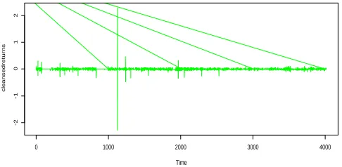
Figure 4: Plot of cleansed log transform of stock returns of GT Bank Plc

Figure 4 above presents the cleansed log transform of the stock returns of the Guaranty Bank Plc from January 2nd_{2001 to May} 8th_{2017. This is done to remove the effects of possible outliers if} any in the financial time series. The analysis of the financial time series in this study will be based on this cleansed series.

Table 1: Summary Statistics of Daily stock Returns of Guaranty Trust Bank Nigeria Plc

Table 1 above examined the characteristics of the financial time series used in this study. The actual stock price, the log transform of the stock price and the log transform of the stock returns exhibited the characteristics of a typical financial time series (i.e evidence of volatility) (Abdulkareem & Abdulkareem, 2016). The series exhibited large standard deviation, skewness and kurtosis. The series further exhibited non-normality using Jarque-Bera Statistic (p-values < 0.05) and shows the presence of ARCH effects (p-values < 0.05), and all the type of series exhibited stationarity at first difference. In addition the averages of the stock series revealed positive values; this implies that the stock price is gaining. With these characteristics revealed above, GARCH and ARMA-GARCH models are appropriate in studying the volatility of the Guaranty Trust Bank stock returns.

ARMA-GARCH Model Performances

Table 2: The Performance of the ARMA (1,1)-GARCH(1,1) Models using Information Criteria with respect to the distributions

In table 2 above, four competing models are compared using student t distribution and skewed student t distribution. The following information criteria such as Akaike, Bayes, Shibata and Hannan-Quinn were used in selecting the preferred model. The results revealed ARMA(1,1)-TGARCH(1,1) as preferred model with the least values of the information criteria using student t and skewed student t distributions.

0 1000 2000 3000 4000

0

1

2

3

Index

lo

g

t

Time

G

T

B

a

n

k

0 1000 2000 3000 4000

-2

-1

0

1

2

Time

cl

e

a

n

se

d

re

tu

rn

s

0 1000 2000 3000 4000

-2

-1

0

1

2

(6)

Modeling and forecasting Daily stock Returns of Guaranty Trust Bank Nigeria Plc

Table 3: The Performance of the ARMA(1,1)-GARCH(2,2)

Models using Information Criteria with respect to the distributions

In table 3 above, four competing models are compared with respect to student t distribution and skewed student t distribution. The following information criteria such as Akaike, Bayes, Shibata and Hannan-Quinn were used in selecting the preferred model. The results revealed ARMA (1,1)-AVGARCH(2,2) is preferred for student t distribution and ARMA(1,1)-TGARCH(2,2)model is preferred for skewed student t distribution.

Persistence and Half-life Volatility of ARMA-GARCH Models

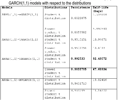
Table 4: The persistence and half-life volatility of the ARMA (1,1)-GARCH(1,1) models with respect to the distributions

Evidence from persistence and half-life volatility in table 4 above shows that the Guaranty Trust Bank stock returns can be modeled and predicted since all the persistence values are all less than 1 (one). ARMA (1,1)-NAGARCH(1,1) exhibited the highest persistence and half-life volatility values while ARMA(1,1)-eGARCH(1,1) exhibited the lowest persistence and half-life volatility values. For all the models, the days of mean-reverting ranges from 5 days to 95 days

Table 5: The persistence and half-life volatility of the ARMA (1,1)-GARCH(2,2) models with respect to the distributions

Evidence from persistence and half-life volatility in table 5 above shows that the Guaranty trust stock returns can be modeled and predicted since all the persistence values are all less than 1 (one). ARMA (1,1)-AVGARCH(2,2) exhibited the highest persistence and half-life volatility values with respect to student t distribution while ARMA(1,1)-NAGARCH(2,2) exhibited the highest persistence and half-life volatility values with respect to skew student t distribution. The ARMA (1,1)-TGARCH(2,2) exhibited the lowest persistence and half-life volatility values for both distributions under consideration. For all the models, the days of mean-reverting ranges from 10 days to 60 days.

Backtesting Evaluation of the Estimated ARMA-GARCH Models

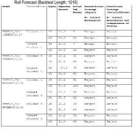
Table 6: Backtesting of the ARMA (1,1)-GARCH(1,1): GARCH Roll Forecast (Backtest Length: 1016)

(7)

Modeling and forecasting Daily stock Returns of Guaranty Trust Bank Nigeria Plc

Backtesting approach is a means to select and use financial

GARCH models for real life application. This approach revealed ARMA(1,1)-eGARCH(1,1) as good model irrespective of the distribution but only failed at 1% alpha level in student t distribution, while other models failed the Backtesting Furthermore, coefficients of the ARMA(1,1)-eGARCH(1,1) model for

both distributions (see Tables 8 and 9 at the appendix) are more significant when compared to the other models (that is, ARMA(1,1)-TGARCH(1,1); ARMA(1,1)-NAGARCH(1,1) and ARMA(1,1)-AVGARCH(1,1)) (see Tables 10 to 15 at the appendix). These results led to the consideration of higher order GARCH model as ARMA (1,1)-GARCH(2,2) models.

Table 7: Backtesting of the ARMA(1,1)-GARCH(2,2): GARCH Roll Forecast (Backtest Length: 1016)

Backtesting approach revealed ARMA(1,1)-eGARCH(2,2) as good model irrespective of the distribution at 1% and 5% alpha levels, while other models failed the Backtesting. Furthermore, coefficients of the ARMA(1,1)-eGARCH(2,2) model for both distributions are more significant (see Tables 16 and 17 at appendix) when compared to the other models (that is, ARMA(1,1)-TGARCH(2,2); ARMA(1,1)-NAGARCH(2,2) and ARMA(1,1)-AVGARCH(2,2)) see Tables 18 to 23 in the Appendix.

DISCUSSION

The log transform of the Guaranty Trust Bank stock returns exhibited the characteristics of a typical financial time series that is evidence of volatility (Abdulkareem & Abdulkareem, 2016) as shown in Table 1. The series exhibited large standard deviation, skewness and kurtosis. The series further exhibited non-normality using Jarque-Bera Statistic (p-values<0.05), shows the presence of ARCH effects (p-values<0.05) and the series exhibited stationarity at first difference. In addition the average value of the returns revealed a positive value which implies that the stock price is gaining (Kuhe, 2018). With these characteristics of the stock returns, the GARCH and ARMA-GARCH models are

appropriate in studying the volatility of the Guaranty Trust Bank stock returns (Emenike & Ani, 2014; Ahmed et al., 2018). In table 2, the four competing models were compared using student t distribution and skewed student t distribution. The following information criteria: Akaike, Bayes, Shibata and Hannan-Quinn were used to select the preferred model. The results revealed ARMA(1,1)-TGARCH(1,1) as preferred model with the least values of the information criteria for both student t and skew student t distributions.

In table 3, the four competing models of higher order were compared with respect to student t distribution and skewed student t distribution. The following information criteria: Akaike, Bayes, Shibata and Hannan-Quinn were employed to select the preferred model. The results revealed ARMA(1,1)-AVGARCH(2,2) is preferred for student t distribution and ARMA(1,1)-TGARCH(2,2)model is preferred for skew student t distribution. Evidence from persistence and half-life volatility in table 4 shows that the Guaranty Trust Bank stock returns can be modeled and predicted since all the persistence values are all less than 1. This also means that the models ensure positive conditional variance as well as stationarity (Banerjee & Sarkar, 2006; Ahmed et al., 2018). The ARMA(1,1)-NAGARCH(1,1) exhibited the highest persistence and half-life volatility values while ARMA(1,1)-eGARCH(1,1) exhibited the lowest persistence and half-life volatility values for both distributions. For all the models, the days of mean-reverting ranges from 5 days to 95 days (that is within three (3) months).

Evidence from persistence and half-life volatility in table 5 shows that the Guaranty Trust Bank stock returns can be modeled and predicted since all the persistence values are all less than 1. This also means that the models ensured positive conditional variance as well as stationary (Banerjee & Sarkar, 2006; Ahmed et al., 2018). ARMA(1,1)-AVGARCH(2,2) exhibited the highest persistence and half-life volatility values with respect to student t distribution while ARMA(1,1)-NAGARCH(2,2) exhibited the highest persistence and half-life volatility values with respect to skewed student t distribution. The ARMA(1,1)-TGARCH(2,2) exhibited the lowest persistence and half-life volatility values for both distributions under consideration. For all the models, the days of mean-reverting ranges from 10 days to 60 days.

Backtesting approach is a means to select and use financial GARCH models for real life application. This approach revealed ARMA(1,1)-eGARCH(1,1) as good model for both distributions but only failed the Conditional Coverage (Christoffersen), this is Correct Exceedances and independence of Failure at 1% alpha level in student t distribution. This contradicts the results from the information criteria that selected ARMA(1,1)-TGARCH(1,1) as the preferred model. This suggests that models should not be selected by information criteria alone but should be selected in addition by how significant the coefficients of the model are, and possibly by backtesting approach (Christoffersen 1998; Christoffersen & Pelletier 2004; Nieppola 2009). The other models under considerations failed the Backtesting. Furthermore, coefficients of the ARMA(1,1)-eGARCH(1,1) model for both distributions (see Tables 8 and 9 in Appendix) are more significant when compared to the other models (that is, ARMA(1,1)-TGARCH(1,1); ARMA(1,1)-NAGARCH(1,1) and ARMA(1,1)-AVGARCH(1,1)) (see Tables 10 to 15 in Appendix). These results led the study to consider higher order GARCH

(8)

Modeling and forecasting Daily stock Returns of Guaranty Trust Bank Nigeria Plc

model as ARMA(1,1)-GARCH(2,2) models which is in line with

Starica (2003), and Hansen & Lunde (2005) that opined that the GARCH(1,1) was clearly inferiors to models that can accommodate a leverage effect. But our results contradicts the work of Namugaya et al. (2014) that GARCH(1.1) outperformed the higher order of GARCH models, this could be because their work did not consider how good is their model.

Backtesting approach revealed ARMA(1,1)-eGARCH(2,2) in Table 7 as good model in respective of the distribution at 1% and 5% alpha levels, while other models failed the Backtesting. Furthermore, coefficients of the ARMA(1,1)-eGARCH(2,2) model for both distributions (see Tables 16 and 17 in Appendix) are more significant than those of the other models (that is, ARMA(1,1)-TGARCH(2,2); ARMA(1,1)-NAGARCH(2,2) and ARMA(1,1)-AVGARCH(2,2)) (see Tables 18 to 23 in Appendix). As mention earlier, ARMA(1,1)-eGARCH(2,2) was selected because it completely passed the backtesting though ARMA(1,1)-AVGARCH(2,2) was selected by information criteria. This suggests model should not be selected by information criteria lone but should be selected in addition, by how significant the coefficients of the model are, and possibly by backtesting approach (Christoffersen, 1998; Nieppola, 2009). Lastly, in all the models considered, there were no ARCH effects in the residuals of the estimated models.

Conclusion and Recommendations

This study revealed that the models considered ensured positive conditional variance as well as stationary (Banerjee & Sarkar, 2006; Ahmed et al., 2018). The study further revealed that using the lowest information criteria values only could not be enough to select preferred GARCH model rather we should add the use of backtesing. The models fitted exhibited high persistency in the daily stock returns and the results further revealed ARMA(1,1)-eGARCH (2,2) model with student t distribution provides a suitable model for evaluating the GT bank stock returns among the competing models. This study recommended that researchers should adopt backtesting approach while fitting GARCH models while the GT bank stock returns has the ability to return to its mean price returns.

REFERENCES

Abdulkareem, A & Abdulkareem, K A 2016, ‘Analyzing Oil Price-Macroeconomic Volatility in Nigeria’, CBN Journal of Applied Statistics, 7(1a):1-22.

Adekeye KS & Aiyelabegan AB 2006, ‘Fitting an ARIMA Model to Experimental Data. Nigerian Statistical Association (NSA) Conference Proceedings, pp. 65 72.

Adenomon, MO 2017a, Introduction to Univariate and Multivariate Time Series Analysis with Examples in R, University Press Plc., Ibadan Nigeria

Adenomon, M 2017b, ‘Modelling and Forecasting Unemployment Rates in Nigeria Using ARIMA Model’, FUW Trends in Science & Technology Journal, 2(1B): 525-531.

Ahmed, RR. Vveinhardt, J, Streimikiene, D & Channar, ZA 2018, ‘Mean Reversion in International Markets: Evidence from GARCH and Half-Life Volatility Models’, Economic Research, 31(1): 1198-1217.

Ali, G 2013 ‘EGARCH, GJR-GARCH, TGARCH, AVGARCH, NGARCH, IGARCH, and APARCH Models for Pathogens at Marine Recreational Sites’, Journal of Statistical and Econometric Methods, 2 (3): 57-73.

Banerjee, A & Sarkar, S 2006, ‘Modeling daily volatility of the Indian stock market using intraday data’, Working Paper No. 588, IIM, Calcutta. Retrieved March 1, 2017, from http://www.iimcal. ac.in/res/upd%5CWPS%20588.pdf Box, GEP & Jenkins GM 1970, Time Series Analysis, Forecasting

and Control. Holden-Day, San Francisco.

Caporale, GM & Pittis, N 2001, ‘Persistence in Macro Economic Time Series: Is it a Model Invariant Property?’, Revista De Economia Del Rosario, 4:117-142.

Christoffersen, P 1998, ‘Evaluating Interval Forecasts’,

International Economic Review, 39: 841– 862.

Christoffersen, P & Pelletier, D 2004, ‘Backtesting value-at-risk: A duration-based approach’, Journal of Financial Econometrics, 2(1): 84–108.

Christoﬀersen, P, Jacobs, K, Ornthanalai, C & Wang, Y 2008, ‘Option valuation with long- run and short-run volatility components’, Journal of Financial Economics, 90: 272-297. Chu, J, Chan, S, Nadarajah, S & Osterrieder, J 2017, ‘GARCH

Modeling of Cryptocurrencies’, Journal of Risk and Financial Management, 10(17):1-15

Cooray, TMJA 2008, Applied Time series Analysis and Forecasting. Narosa Publishing House , New Delhi.. Dhamija, A & Bhalla, VK 2010, ‘Financial time series forecasting:

comparison of neural Networks and ARCH models’,

International Research Journal of Finance and Management, 49 (1): 159-172

Dobre, I & Alexandru, AA 2008, ‘Modelling Unemployment Rate using Box-Jenkins Procedure’, Journal of Applied Quantitative Methods. 3(2): 156-166.

Emenike, KO, & Ani, WU 2014, ‘Volatility of the Banking Sector Returns in Nigeria. Ruhuna’, Journal of Management and Finance, 1(1): 73-82.

Emenogu, NG, & Adenomon, MO 2018, ‘The Effect of High Positive Autocorrelation on the Performance of GARCH

Family Models’, Preprints.

doi:10.20944/preprints201811.0381.v1

Emenogu, NG, Adenomon, MO & Nweze, NO, 2018, ‘On The Volatility of Daily Stock Returns of Total Petroleum Company of Nigeria: Evidence from GARCH Models, Value-at-Risk and Backtesting’, Preprints, doi:10.20944/preprints201812.0043.v1

Enders, W 2004, Applied Econometric Time Series, New York, John Wiley.

Engle, RF & Patton, AJ 2001, ‘What Good is Volatility Model?’,

Quantitative Finance, 1: 237-245.

Engle, R,& Rangel, J 2008, ‘The spline-GARCH model for low-frequency volatility and its global macroeconomic causes’

Review of Financial Studies, 21: 1187-1222.

Enocksson, D & Skoog, J 2012, Evaluating VaR (Value-at-Risk): with the ARCH/GARCH class models via, Lambert Academic Publishing (LAP), European Union.

Ghalanos, A 2018, Package ‘rugarch’. R Team Cooperation. Grek, A 2014, ‘Forecasting accuracy for ARCH models and

GARCH(1,1) family which model does best capture the volatility of the Swedish stock market?’, Statistics Advance Level Theses 15hp; Örebro University.

Grigoletto, M & Lisi, F 2009, ‘Looking for Skewness in Financial Time Series’, The Econometrics Journal, 12(2): 310-323. Gujarati, DN 2003, Basic Econometrics, 4th_{edn. New Delhi, The}

McGraw-Hill Co.

(9)

Modeling and forecasting Daily stock Returns of Guaranty Trust Bank Nigeria Plc

Hall, P, & Yao, P 2003, ‘Inference in ARCH and GARCH Models

with Heavy-Tailed Errors’, Econometrica, 71: 285-317. Hansen, PR & Lunde, A 2005, ‘A Forecast Comparison of

Volatility Models: Does Anything Beat a GARCH (1,1)?’,

Journal of Applied Econometrics, 20: 873-889.

Heracleous, MS 2003, ‘Volatility Modeling Using the Student’s t Distribution’, Ph.D Thesis, Virginia Polytechnic Institute and State University, Blacksburg, Virginia.

Jiang, W 2012, ‘Using the GARCH model to analyse and predict the different stock markets’, Master Thesis in Statistics, Department of Statistics, Uppsala University Sweden.

Kirchgässner, G & Wolters, J 2017, Introduction to Modern Time Series Analysis, New York, Springer Books.

Kongcharoen, C & Kruangpradit, T 2013, ‘Autoregressive Integrated Moving Average with Explanatory Variable (ARIMAX) Model for Thailand Export’, A paper presented at the 33rd_{International Symposium on Forecasting, South} Korea, June 2013.

Kuhe, DA 2018, ‘Modeling Volatility Persistence and Asymmetry with Exogenous Breaks in the Nigerian Stock Returns’,

CBN Journal of Applied Statistics, 9(1): 167-196.

Lange, T 2011, ‘Tail Behavior and OLS Estimating in AR-GARCH Models’, Statistica Sinica, 21(3): 1191-1200.

Lawrance, AJ 2013, ‘Exploration Graphics for Financial Time Sewries Volatility’, Journal of the Royal Statistical Society Series C (Applied Statistics), 62(5): 669-686. Magnus, FJ & Fosu, AE 2006, ‘Modelling and Forecasting

Volatility of Returns on the Ghana Stock Exchange Using GARCH Models’, Am. J. Appl. Sci., 3(10): 2042-2048. Marra, S 2015, ‘Predicting Volatility’, Investment Research.

LAZARD Asset Management (LR26017), Australia. Namugaya, J, Weke, P & Charles WM 2014, ‘Modelling Stock

Returns Volatility on Uganda Securities Exchange’, Applied Mathematical Science, 8: 5173-5184.

Nelson, D 1991, ‘Conditional heteroskedasticity in asset pricing: A new approach’, Econometrica, 59, 347-370.

Nieppola, O 2009, ‘Backtesting Value-at-Risk Models’, M.Sc. Thesis, Helsinki School of Economics, Finland.

Panait, I & Slavescu, EO 2012, ‘Using GARCH-in-Mean Model to Investigate Volatility and Persistence at Different Frequencies for Bucharest Stock Exchange During 1997-2012’, Theoretical and Applied Economics, 19(5): 55-76. Pedroni, P 2001, ‘The Econometric Modeling of Financial Time

Series by Terence Mills’, Journal of the American Statistical Association, 96(453): 345-346.

Peterson, BG, Carl, P, Boudt, K, Bennett, R, Ulrich, J, Zivot, E, Cornilly, D, Hung, E, Lestel, M, Balkissoon, K & Wuertz, D 2018, Package ‘PerformanceAnalytics’. R Team Cooperation

Ruppert, D 2011, Statistics and Data Analysis for Financial Engineering, Springer Science + Business Media, New York.

Sahai, AK 2016, ‘Volatility Modelling and Forecasting Efficiency of GARCH Models on Soy Oil Futures in India and the US’,

Journal of Energy Technology and Policy, 6(3): 32-38. Starica, C 2003, ‘Is GARCH (1,1) as Good a Model as the Nobel

Prize Accolades would Imply?’ www.math.chalmers.se/starica downloaded on 27-02-2019 Summinga-Sonagadu, R and Narsoo, J. 2019, Risk Model

Validation: An Intraday VaR and ES Approach Using the

Multiplicative Component GARCH. Risks, 7, 10; doi:10.3390/risks7010010

Tay, H-Z; Ng, K-H; Koh, Y-B. and Ng, K-H. 2019, Model Selection Based on Value-at-Risk Backtesting Approach for GARCH-Type Models. Journal of Industrial and Management Optimization, doi:10.3934/jimo.2019021

Tsay, RS 2005, Analysis of financial time series, 2nd edn. John Wiley & Sons, New Jersey.

Usman, U, Auwal, HM, & Abdulmuhyi, MA 2017, ‘Fitting the Nigeria Stock Returns Using GARCH Models’, Theoretical Economics Letters, 7: 2159-2176.

Vosvrda, M 2006, ‘Empirical Analysis of Persistence and Dependence Patterns Among the Capital Markets’, Prague Economic Papers, 3: 231-242.

Wilhelmsson, A 2006, ‘GARCH Forecasting Performance under Different Distribution Assumptions’, Journal of Forecasting, 25: 561-578.

Appendix

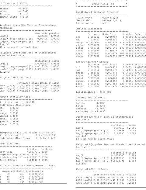
Table 8: Estimates of ARMA(1,1)-eGARCH(1,1) with std *---* * GARCH Model Fit * *---* Conditional Variance Dynamics --- GARCH Model : eGARCH(1,1) Mean Model : ARFIMA(1,0,1) Distribution : std

Optimal Parameters

--- Estimate Std. Error t value Pr(>|t|)

ar1 0.090426 0.135239 0.66864 0.503724

ma1 0.015825 0.133828 0.11825 0.905871

omega -0.638445 0.020334 -31.39719 0.000000

alpha1 0.192669 0.052765 3.65144 0.000261

beta1 0.882287 0.001346 655.31371 0.000000

gamma1 1.831176 0.019753 92.70358 0.000000

shape 2.100000 0.009205 228.12482 0.000000

Robust Standard Errors:

Estimate Std. Error t value Pr(>|t|)

ar1 0.090426 0.143390 0.63063 0.52828

ma1 0.015825 0.149513 0.10584 0.91571

omega -0.638445 0.081165 -7.86604 0.00000

alpha1 0.192669 0.171535 1.12321 0.26135

beta1 0.882287 0.002625 336.12545 0.00000

gamma1 1.831176 0.357599 5.12075 0.00000

shape 2.100000 0.049998 42.00152 0.00000

(10)

Modeling and forecasting Daily stock Returns of Guaranty Trust Bank Nigeria Plc

LogLikelihood : 9737.114

Information Criteria

--- Akaike -4.8457

Bayes -4.8347 Shibata -4.8457 Hannan-Quinn -4.8418

Weighted Ljung-Box Test on Standardized Residuals

--- statistic p-value Lag[1] 0.06633 0.7968 Lag[2*(p+q)+(p+q)-1][5] 0.08466 1.0000 Lag[4*(p+q)+(p+q)-1][9] 0.23001 1.0000 d.o.f=2

H0 : No serial correlation

Weighted Ljung-Box Test on Standardized Squared Residuals

Weighted ARCH LM Tests

--- Statistic Shape Scale P-Value ARCH Lag[3] 0.0004649 0.500 2.000 0.9828 ARCH Lag[5] 0.0011178 1.440 1.667 1.0000 ARCH Lag[7] 0.0016103 2.315 1.543 1.0000

Nyblom stability test

--- Joint Statistic: 10.9421

Individual Statistics: ar1 1.2313

ma1 1.2554 omega 2.7533 alpha1 0.8187 beta1 2.1565 gamma1 0.6688 shape 0.2326

Asymptotic Critical Values (10% 5% 1%) Joint Statistic: 1.69 1.9 2.35 Individual Statistic: 0.35 0.47 0.75

Sign Bias Test

--- t-value prob sig Sign Bias 0.98272 0.3258 Negative Sign Bias 0.33742 0.7358 Positive Sign Bias 0.02935 0.9766 Joint Effect 1.04044 0.7915

Adjusted Pearson Goodness-of-Fit Test: --- group statistic p-value(g-1) 1 20 852 1.903e-168 2 30 1131 1.637e-219 3 40 1420 7.300e-273 4 50 1694 7.905e-323

Table 9: Estimates of ARMA(1,1)-eGARCH(1,1) with sstd *---* * GARCH Model Fit * *---*

Conditional Variance Dynamics --- GARCH Model : eGARCH(1,1) Mean Model : ARFIMA(1,0,1) Distribution : sstd

Optimal Parameters

---

Estimate Std. Error t value Pr(>|t|) ar1 0.090252 0.059767 1.51006 0.131029 ma1 0.013462 0.058206 0.23129 0.817091 omega -0.355651 0.021578 -16.48217 0.000000 alpha1 0.617628 0.165270 3.73708 0.000186 beta1 0.885358 0.004641 190.76635 0.000000 gamma1 5.501824 0.189529 29.02895 0.000000 skew 1.000633 0.009679 103.38505 0.000000 shape 2.010000 0.000613 3278.52434 0.000000

Estimate Std. Error t value Pr(>|t|) ar1 0.090252 0.038433 2.34831 0.018859 ma1 0.013462 0.025677 0.52431 0.600066 omega -0.355651 0.091076 -3.90499 0.000094 alpha1 0.617628 0.518456 1.19128 0.233542 beta1 0.885358 0.026923 32.88446 0.000000 gamma1 5.501824 0.598899 9.18656 0.000000 skew 1.000633 0.007893 126.77568 0.000000 shape 2.010000 0.001837 1094.18647 0.000000

--- Akaike -4.8480

Bayes -4.8354 Shibata -4.8480 Hannan-Quinn -4.8435

(11)

Modeling and forecasting Daily stock Returns of Guaranty Trust Bank Nigeria Plc

ma1 1.2345 omega 2.6897 alpha1 0.9021 beta1 1.7730 gamma1 0.6292 skew 0.1230 shape 0.2369

Sign Bias Test

Adjusted Pearson Goodness-of-Fit Test: --- group statistic p-value(g-1) 1 20 961.4 9.289e-192 2 30 1308.9 2.714e-257 3 40 1647.1 7.026e-321 4 50 1970.2 0.000e+00

Table 10: Estimates of ARMA (1,1)-TGARCH(1,1) with std *---* * GARCH Model Fit * *---*

Conditional Variance Dynamics --- GARCH Model : fGARCH(1,1) fGARCH Sub-Model : TGARCH Mean Model : ARFIMA(1,0,1) Distribution : std

Optimal Parameters

---

Estimate Std. Error t value Pr(>|t|) ar1 0.260521 0.018296 14.23931 0.00000 ma1 -0.111401 0.018403 -6.05358 0.00000 omega 0.000000 0.000000 0.18102 0.85635 alpha1 0.695885 0.015610 44.58006 0.00000 beta1 0.499255 0.008670 57.58337 0.00000 eta11 -0.005608 0.021908 -0.25598 0.79797 shape 3.117434 0.057788 53.94586 0.00000

Estimate Std. Error t value Pr(>|t|) ar1 0.260521 0.327748 0.794880 0.426683 ma1 -0.111401 0.423033 -0.263339 0.792289 omega 0.000000 0.000065 0.000551 0.999560 alpha1 0.695885 2.953122 0.235644 0.813709 beta1 0.499255 2.233770 0.223503 0.823144 eta11 -0.005608 0.246792 -0.022723 0.981871 shape 3.117434 1.074083 2.902415 0.003703

---

Akaike -6.0027 Bayes -5.9917 Shibata -6.0027 Hannan-Quinn -5.9988

Weighted Ljung-Box Test on Standardized Residuals ---

statistic p-value Lag[1] 2.709e-10 1 Lag[2*(p+q)+(p+q)-1][5] 2.575e-08 1 Lag[4*(p+q)+(p+q)-1][9] 5.878e-08 1 d.o.f=2

ma1 0.1850 omega 127.6935 alpha1 65.3278 beta1 8.8435 eta11 1.1637 shape 3.4515

Sign Bias Test

Adjusted Pearson Goodness-of-Fit Test: --- group statistic p-value(g-1) 1 20 855.3 3.746e-169 2 30 1208.4 6.256e-236 3 40 1450.8 2.785e-279 4 50 1752.6 0.000e+00

(12)

Modeling and forecasting Daily stock Returns of Guaranty Trust Bank Nigeria Plc

Table 11: Estimates of ARMA(1,1)-TGARCH(1,1) with sstd

*---* * GARCH Model Fit * *---*

Conditional Variance Dynamics --- GARCH Model : fGARCH(1,1) fGARCH Sub-Model : TGARCH Mean Model : ARFIMA(1,0,1) Distribution : sstd

Optimal Parameters

---

Estimate Std. Error t value Pr(>|t|) ar1 0.217562 0.036887 5.89804 0.00000 ma1 -0.054003 0.036536 -1.47808 0.13939 omega 0.000000 0.000000 0.17964 0.85743 alpha1 0.732986 0.016282 45.01939 0.00000 beta1 0.474753 0.008953 53.02883 0.00000 eta11 0.007986 0.021498 0.37149 0.71027 skew 1.003418 0.011781 85.17358 0.00000 shape 3.107679 0.056652 54.85523 0.00000

---

statistic p-value Lag[1] 3.349e-08 0.9999 Lag[2*(p+q)+(p+q)-1][5] 1.764e-07 1.0000 Lag[4*(p+q)+(p+q)-1][9] 3.366e-07 1.0000 d.o.f=2

ma1 0.16059 omega 131.29433 alpha1 68.81920 beta1 10.30766 eta11 1.58122 skew 0.05679 shape 3.51394

Sign Bias Test

Adjusted Pearson Goodness-of-Fit Test: --- group statistic p-value(g-1) 1 20 960 1.798e-191 2 30 1290 3.095e-253 3 40 1638 5.095e-319 4 50 1936 0.000e+00

Table 12: Estimates of ARMA(1,1)-NAGARCH(1,1) with std *---* * GARCH Model Fit * *---*

Conditional Variance Dynamics --- GARCH Model : fGARCH(1,1) fGARCH Sub-Model : NAGARCH Mean Model : ARFIMA(1,0,1) Distribution : std

Optimal Parameters

---

Estimate Std. Error t value Pr(>|t|) ar1 0.202254 0.161208 1.25462 0.20962 ma1 -0.136256 0.166396 -0.81887 0.41286 omega 0.000000 0.000000 0.11911 0.90519 alpha1 0.348048 0.012211 28.50355 0.00000 beta1 0.643824 0.009687 66.46287 0.00000 eta21 0.043594 0.089369 0.48779 0.62570 shape 3.715735 0.102281 36.32859 0.00000

Estimate Std. Error t value Pr(>|t|) ar1 0.202254 0.414763 0.48764 0.625807 ma1 -0.136256 0.515821 -0.26415 0.791661 omega 0.000000 0.000073 0.00049 0.999609 alpha1 0.348048 1.863233 0.18680 0.851819 beta1 0.643824 1.833290 0.35119 0.725450 eta21 0.043594 0.332024 0.13130 0.895540 shape 3.715735 1.523823 2.43843 0.014751

(13)

Modeling and forecasting Daily stock Returns of Guaranty Trust Bank Nigeria Plc

---

ma1 0.3992 omega 101.8067 alpha1 51.9765 beta1 7.8753 eta21 1.3598 shape 4.1795

Sign Bias Test

Adjusted Pearson Goodness-of-Fit Test: --- group statistic p-value(g-1) 1 20 1161 2.433e-234 2 30 1491 4.173e-296 3 40 1744 0.000e+00 4 50 1987 0.000e+00

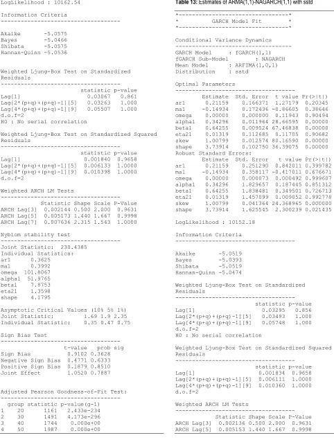
Table 13: Estimates of ARMA(1,1)-NAGARCH(1,1) with sstd

Conditional Variance Dynamics --- GARCH Model : fGARCH(1,1) fGARCH Sub-Model : NAGARCH Mean Model : ARFIMA(1,0,1) Distribution : sstd

Optimal Parameters

---

Estimate Std. Error t value Pr(>|t|) ar1 0.21159 0.166371 1.27179 0.20345 ma1 -0.14934 0.172436 -0.86605 0.38646 omega 0.00000 0.000000 0.11943 0.90494 alpha1 0.34296 0.011964 28.66595 0.00000 beta1 0.64255 0.009524 67.46838 0.00000 eta21 0.01319 0.112685 0.11705 0.90682 skew 1.00799 0.012574 80.16590 0.00000 shape 3.73914 0.102750 36.39075 0.00000 Robust Standard Errors:

---

--- Statistic Shape Scale P-Value ARCH Lag[3] 0.002136 0.500 2.000 0.9631 ARCH Lag[5] 0.005153 1.440 1.667 0.9998

(14)

Modeling and forecasting Daily stock Returns of Guaranty Trust Bank Nigeria Plc

ARCH Lag[7] 0.007607 2.315 1.543 1.0000

ma1 0.41837 omega 101.51981 alpha1 55.11488 beta1 8.72212 eta21 0.65460 skew 0.07016 shape 4.15469

Sign Bias Test

Adjusted Pearson Goodness-of-Fit Test: --- group statistic p-value(g-1) 1 20 1255 1.619e-254 2 30 1659 0.000e+00 3 40 1917 0.000e+00 4 50 2194 0.000e+00

Table 14: Estimates of ARMA(1,1)-AVGARCH(1,1) with std

Conditional Variance Dynamics --- GARCH Model : fGARCH(1,1) fGARCH Sub-Model : AVGARCH Mean Model : ARFIMA(1,0,1) Distribution : std

Optimal Parameters

---

Estimate Std. Error t value Pr(>|t|) ar1 0.216232 0.020440 10.57901 0.000000 ma1 -0.091422 0.022696 -4.02803 0.000056 omega 0.000000 0.000000 0.17852 0.858313 alpha1 0.722956 0.015914 45.42756 0.000000 beta1 0.476527 0.008804 54.12823 0.000000 eta11 -0.026953 0.021307 -1.26499 0.205876 eta21 0.000193 0.001045 0.18441 0.853692 shape 3.141671 0.058494 53.70923 0.000000

Estimate Std. Error t value Pr(>|t|) ar1 0.216232 0.228626 0.945789 0.344256 ma1 -0.091422 0.543642 -0.168165 0.866453 omega 0.000000 0.000068 0.000531 0.999576 alpha1 0.722956 2.763034 0.261653 0.793589 beta1 0.476527 2.080736 0.229018 0.818855 eta11 -0.026953 0.287347 -0.093800 0.925268

eta21 0.000193 0.002573 0.074930 0.940270 shape 3.141671 1.430933 2.195539 0.028125

---

ma1 0.4489 omega 130.6555 alpha1 69.7212 beta1 11.1180 eta11 0.5819 eta21 0.3538 shape 3.9707

Sign Bias Test

Adjusted Pearson Goodness-of-Fit Test: --- group statistic p-value(g-1) 1 20 961 1.130e-191 2 30 1315 1.142e-258 3 40 1572 5.360e-305

(15)

Modeling and forecasting Daily stock Returns of Guaranty Trust Bank Nigeria Plc

4 50 1898 0.000e+00

*---*

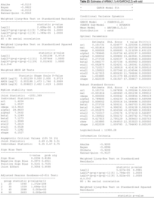
Table 15: Estimates of ARMA(1,1)-AVGARCH(1,1) with sstd * GARCH Model Fit * *---*

Conditional Variance Dynamics --- GARCH Model : fGARCH(1,1) fGARCH Sub-Model : AVGARCH Mean Model : ARFIMA(1,0,1) Distribution : sstd

Optimal Parameters

---

Estimate Std. Error t value Pr(>|t|) ar1 0.186919 0.052008 3.59404 0.000326 ma1 -0.044629 0.054695 -0.81596 0.414520 omega 0.000000 0.000000 0.18133 0.856108 alpha1 0.603595 0.013305 45.36510 0.000000 beta1 0.535856 0.008274 64.76511 0.000000 eta11 -0.023806 0.021919 -1.08608 0.277441 eta21 0.000161 0.001017 0.15863 0.873957 skew 1.008536 0.012038 83.78155 0.000000 shape 3.330057 0.069111 48.18388 0.000000

Estimate Std. Error t value Pr(>|t|) ar1 0.186919 0.754665 0.247684 0.80438 ma1 -0.044629 0.299470 -0.149028 0.88153 omega 0.000000 0.000064 0.000561 0.99955 alpha1 0.603595 2.862902 0.210833 0.83302 beta1 0.535856 2.346030 0.228410 0.81933 eta11 -0.023806 0.347020 -0.068602 0.94531 eta21 0.000161 0.000145 1.112047 0.26612 skew 1.008536 0.025408 39.693201 0.00000 shape 3.330057 2.369263 1.405524 0.15987

---

ma1 0.17936 omega 119.81614 alpha1 71.63048 beta1 9.27011 eta11 0.99530 eta21 0.63851 skew 0.05967 shape 4.18341

Sign Bias Test

Adjusted Pearson Goodness-of-Fit Test: --- group statistic p-value(g-1) 1 20 1035 1.779e-207 2 30 1371 2.107e-270 3 40 1672 0.000e+00 4 50 2011 0.000e+00

Table 16: Estimates of ARMA(1,1)-eGARCH(2,2) with std *---* * GARCH Model Fit * *---*

Conditional Variance Dynamics --- GARCH Model : eGARCH(2,2) Mean Model : ARFIMA(1,0,1) Distribution : std

Optimal Parameters

---

Estimate Std. Error t value Pr(>|t|) ar1 0.68786 0.014697 46.8036 0 ma1 -0.53668 0.015623 -34.3512 0 omega -0.25233 0.001059 -238.2264 0 alpha1 0.39354 0.053218 7.3948 0 alpha2 -0.52520 0.002786 -188.5413 0 beta1 0.73683 0.000159 4631.2482 0 beta2 0.23768 0.000247 963.5852 0 gamma1 3.69469 0.006275 588.8134 0 gamma2 0.44676 0.002619 170.5717 0 shape 2.10000 0.000751 2797.4873 0

Estimate Std. Error t value Pr(>|t|) ar1 0.68786 0.048823 14.089 0.00000

(16)

Modeling and forecasting Daily stock Returns of Guaranty Trust Bank Nigeria Plc

ma1 -0.53668 0.040005 -13.415 0.00000

omega -0.25233 0.004415 -57.147 0.00000 alpha1 0.39354 0.241286 1.631 0.10289 alpha2 -0.52520 0.003159 -166.235 0.00000 beta1 0.73683 0.002479 297.207 0.00000 beta2 0.23768 0.002884 82.418 0.00000 gamma1 3.69469 0.073306 50.401 0.00000 gamma2 0.44676 0.004863 91.866 0.00000 shape 2.10000 0.003104 676.648 0.00000

---

statistic p-value Lag[1] 0.0006631 0.9795 Lag[2*(p+q)+(p+q)-1][5] 0.0019914 1.0000 Lag[4*(p+q)+(p+q)-1][9] 0.0033223 1.0000 d.o.f=2

-