Model-based Bayesian Reinforcement Learning in Factored Markov Decision Process

Model-based Bayesian Reinforcement Learning

in Factored Markov Decision Process

Bo Wu

Education Technology and Information Center, Shenzhen Polytechnic, Shenzhen, China Email: wubo@szpt.edu.cn

Yanpeng Feng and Hongyan Zheng

Education Technology and Information Center, Shenzhen Polytechnic, Shenzhen, China Email: {zhenghongyan, ypfeng}@szpt.edu.cn

Abstract—Learning the enormous number of parameters is a challenging problem in model-based Bayesian reinforcement learning. In order to solve the problem, we propose a model-based factored Bayesian reinforcement learning (F-BRL) approach. F-BRL exploits a factored representation to describe states to reduce the number of parameters. Representing the conditional independence relationships between state features using dynamic Bayesian networks, F-BRL adopts Bayesian inference method to learn the unknown structure and parameters of the Bayesian networks simultaneously. A point-based online value iteration approach is then used for planning and learning online. The experimental and simulation results show that the proposed approach can effectively reduce the number of learning parameters, and enable online learning for dynamic systems with thousands of states.

Index Terms—Markov Decision Processes (MDP), Bayesian Reinforcement Learning (BRL), Dynamic Bayesian Networks (DBNs), Curse of Dimensionality

I. INTRODUCTION

Learning dynamical systems based on Markov decision process (MDP) or partially observable Markov decision process (POMDP) is an interdisciplinary research area of machine learning, control theory, and operations research. The main objective in this research area is to realize data-driven multi-stage optimal control for complex or uncertain dynamical systems [1-3]. Intelligent agent must learn by interacting with its environment to achieve a goal. Reinforcement learning (RL) is an effective learning method of the optimal control system under complex and uncertain environment. One of the challenges that arises in reinforcement learning and not in other learning tasks is the trade-off between exploration and exploitation [4, 5]. Exploration and exploitation are complementary, but opposite to each other. Exploration leads to the maximization of the gain in the long run at the risk of losing short term reward, while exploitation maximizes the short term gain at the price of losing the gain over the long run [6]. The dilemma is that neither exploration nor exploitation can be pursued exclusively without failing the task [7].

Bayesian reinforcement learning (BRL) utilizes prior knowledge to model the unknown parameters, updates the posterior distribution of the unknown parameters according to observation data, and finally plans using the posterior distribution to maximize the expected reward [8]. BRL transforms the learning problem into a planning problem. Because BRL can use the prior knowledge of states to model the unknown parameters and the unknown structure, it has recently been shown to provide an elegant solution to the exploration and exploitation trade-off in reinforcement learning [9].

BETTLE [9] and PO-BEETLE [10] are the point-based value iteration algorithms adapted to Bayesian reinforcement learning in fully observable domains and in partially observable domains respectively. Ross and Pineau [11] proposed to use a factored representation combined with online planning techniques to learn the learning parameters of a structured dynamical system. Wang et al exploited a Monte Carlo Bayesian reinforcement learning (MC-BRL) [12] method to generalize the approaches in BRL. However, in BRL, the number of the learning parameters is large and grows exponentially with the number of states. Moreover, there is a dimensionality curse to plan over the full space of all possible posteriors. Due to the high complexity of model-based BRL, most approaches have been limited to very small domains, and are unable to achieve online learning in large-scale domains [13].

To address the above issues, we propose a model-based factored online Bayesian reinforcement learning approach. The paper is organized as follows. Section.2 reviews the POMDP formulation of BRL. Section.3 describes the efficient model-based factored online Bayesian reinforcement learning approach. Section.4 empirically demonstrates F-BRL on the Chain problem and RobocupRescue. Section.5 concludes this paper.

II. BAYESIAN REINFORCEMENT LEARNING IN MDP Markov Decision Process (MDP) is represented as a tuple (S, A, T, R). S ={ , , ,..., }s s s1 2 3 sn is the set of all the

environment states which are not directly observable. 1 2 3

{ , , ,..., }

= m

which stochastically affect the states of the world.

( , , ')= ( ' | , )

T s a s P s s a is the state transition probability distribution that represents the probability of ending in state s' if the agent performs action a in state s,

( , , ')=1, ( , )

∈ ∀

∑s S

T s a s s a . R s a s( , , ') is the reward function, which is the reward obtained by executing action a in state s. The objective of MDP planning is to optimize action selection. The goal of the agent is to collect as much reward as possible over time.

In reinforcement learning, the state transition function is an unknown learning parameter sas'

θ . Because the state transition function is a conditional probability distribution, the learning parameter satisfies the following conditions:

'

'

1, [0,1].

∈

⎧ ₌

⎪ ⎨

∈

⎪⎩

∑

sas

s S sas

θ

θ (1)

We can formulate the model-based BRL as a partially observable Markov decision process (POMDP) [13], which is formally described by a tuple

( ,SP A Z T O RP, P, ,P P, P). Here

'

{ }

= × sas P

S S θ is the set of states composed of the cross product of the MDP discrete states s with the continuous unknown parameters θsas'_.

The action space AP is the same as that of the underlying

MDP. The observation space ZP =S is identical to the

MDP states space since it is fully observable. The transition function ( , , , ', ')T sP θ a s θ =P s( ', ' | , , )θ sθ a can be factored into two conditional distributions [9].

' '

( , , , ', ') ( ', ' | , , )

( ' | , , , ') ( ' | , , ) .

= = = P

sas

T s a s P s s a

P s s a P s a θθ

θ θ θ θ

θ θ θ θ

θ δ

(2)

where _δθθ' _{is a Kronecker delta.}

' 1, '

0. otherwise.

=

⎧

=⎨ ⎩

θθ θ θ

δ (3)

Kronecker delta essentially denotes the assumption that the unknown parameters are stationary [9]. The observation function O sP( ', ', , )θ a z =P z s( | ', ', )θ a

indicates the probability of observing z when state s',θ' are reached after executing action a. According to the definition, each observation corresponds to a state, so

' ( | ', ', )₌ s z

P z s θ a δ . Because the reward function is independent of θ and θ' , R sP( , , , ', ')θ a s θ can be

denoted by R s a s( , , ').

According to the definition of BRL, the MDP problem can be transformed into a POMDP problem. In a POMDP, belief b s( ) is the probability distribution over the

unknown states set S. Based on the belief, we can learn the state/observation transition models by belief monitoring approach [14] using the Bayes’ theorem:

'_{( )= ( ) ( ' | , , )= ( )} '_.

sas sas

b θ η θb P s θ s a η θ θb (4) where η is a normalization factor.

Belief monitoring can be performed easily when the prior belief and the posterior distribution belong to the same family of distributions [9]. BRL exploits Dirichlet distribution to represent the prior belief and the posterior distribution. Suppose the prior belief is represented by

,

( )=

_∏

( sa; sa)

s a

bθ Dθ n , where sa

n is the vector of hyper-parameter sas'

n . The posterior distribution is:

' ' '

,

, , ' ,

( ) ( ; )

( ; ( , , ')).

=

= +

∏

∏

sas sas sa sas

s a

sa sa

s a s s a

b D n

D n s a s

θ ηθ θ

θ δ (5)

where δ is a Kronecker delta that equals 1 when s=s,

=

a a, s'=s', and 0 otherwise.

The goal of BRL is to find the optimal policy of the POMDP, which yields an action selection strategy that achieves an optimal tradeoff between exploration and exploitation , and hence maximizes the long term expected return given the current model posterior and state of the agent [11]. In POMDP, the policy π is the mapping from belief b to action a, π( )b →a . The optimal policy _π∗ _{is the policy that yields the optimal} value function _V∗ _{defined by the Bellman equation:} ∗( ) max ( | , ) ( , , ') ∗( ') .

∈ _∈ ⎡ ⎤

=

∑

_⎣ + _⎦

a A _{z Z}

V b P z b a R s a s γV b (6)

where 'b is the next belief.

In BRL, states are partly discrete and partly continuous. Following the definition by Duff [13], the Bellman's equation can be re-written as:

'

'

( ) max ( ' | , , ) ( , , ') ( ) .

∗ ∗

∈ _∈ ⎡ ⎤

=

∑

_⎣ + sas _⎦

a A _{s S}

V b P s s b a R s a s γV b (7)

where b is the current belief, bsas' is the posterior belief, and the observation is state s'.

III. MODEL-BASED BRL IN STRUCTURED DOMAINS The main challenge that arises in BRL is that the number of learning parameters is very huge. The number of learning parameters is proportional to the number of states of dynamic system. When the size of states is very big, in order to obtain a good model under uncertainty, we need to collect a large amount of data during the learning process. The number of learning parameters will grow exponentially. The learning process is unable to achieve rapid convergence. The factored representation is an effective way to solve this curse of dimensionality [15-17]. In this factored representation, if the independent relationships between the state variables in DBNs are given, the learning parameters can be compressed easily. However, because the structure of DBNs is always unknown [18, 19], we must learn the structure and parameters simultaneously.

A. Factored Representation

Let X ={ ,...,X1 Xn} be the set of n random variables that

fully describe a state, each Xi denoting a feature variable

of the state. Let Xi be the set of all possible values of the

random variables in set X. Therefore, a state is defined by assigning a value to each variable

1 1

{ ,..., }

= = n= n

s X x X x , which can be abbreviated as

1

{ }₌

= n

i i

s x with x_i∈X_i . The number of states is

1

| |=

_∏

n₌| | i i

S X . Factored representations can be very

compact when individual actions affect relatively few features, or when their effects exhibit certain regularities [21]. According to the factored representation of states, the state transition function, observation function and reward function can be compactly represented by dynamic Bayesian networks (DBNs).

A DBN is a directed acyclic graph. Its nodes represent state, action and observation variables, and its edges (or arcs) encode the relationship of probability dependencies. Each node is accompanied by a conditional probability table (CPT) to describe the influence of its father nodes. The conditional probability distribution is

( i' | ( i'))

P X parents X . The size of parameters in the CPT is exponential in the number of father nodes. The MDP transform into Factored MDP (FMDP) after deploying factored representation. FMDP breaks down the joint probability distribution into some smaller factors.

Let G a( ) be a two-layer directed acyclic graph with ∈

a A and X ={ , ,X1 Xn,X1', ,Xn'} . Let θG a( ) denote a CPT. The state transition function T can be represented by G a( ) and θG a_{( )} . Let Xi be the ith

variable at the current time step, Xi' be the ith variable

at the next time step. Xi and Xi' share the same

collection of values. Let ( ) ≺

G a i

X be the value of the father nodes under Xi'=xi. Given G a( ) and θG a( ), the state transition function can be calculated by:

( )

1

( , , ') ( , , ')

( ' | , ).

=

=

=

_∏

≺

n

G a

i i

i

T s a s T X a X

P X X a (8)

where T s a s( , , ') is the state transition function without

the factored representation, and T X a X( , , ') is the

factored state transition function.

Consequently, the factored representation can simplify the process of knowledge acquisition and domain modeling, and reduce the complexity of reasoning. We can learn the unknown model by computing the posterior belief repeatedly.

B. Updating Posterior Belief

The process of factored BRL is that the agent interacts with the environment, obtains observation data, learns the unknown parameters and the unknown structure, and thereby estimates the state transition model and reward model. Given the initial belief b s( ) under uncertainty,

the posterior belief can be computed by:

a z, '( ')= ([ ']Z' = ')

∑

( ) ( ' | , ).

S

b s ηδ s z b s P s s a (9)

where η is the normalization factor and [ ']Zs ' is subset of state values corresponding to observation Z'. δ is the

Kronecker function that equals 1 when [ ']s Z' =z' is true, and 0 otherwise. Since the model and structure are unknown, the belief states are updated as follows.

( ) ( ) ( )

( ', G a )= ([ '])

∑

( ' | , , G a ) ( , G a ).

X

b X θ ηδ X P X X aθ b X θ (10)

where X and X' are factored features, a denotes action, Z denotes the set of observation data, z is the subset of Z,

( )

G a

θ is the unknown parameter, and δ is the Kronecker function.

Updating belief states requires historical information. Therefore, this process needs to iterate over every observation and action throughout the history. The enormous computation required makes (10) hard to converge. According to Poupart et al [9], beliefs represented by mixtures of products of Dirichlet distributions are closed under belief updating for factored domains. So we can represent the beliefs as the mixtures of products of Dirichlet distributions. The beliefs prior probability can be represented as the mixtures of products of Dirichlet distributions as follows.

( , ( ))=

∑

,

∏

, ( ( )≺ ).

G i X

G a i X i X G a

i

b X θ c D θ (11)

where ci X, is the coefficient of Dirichlet, D denotes Dirichlet distributions, and ( )≺ = ( ' | ( '))

G i X

G a P X parents X

θ .

The belief posterior probability after belief updating can be computed as follows.

, '( ', ( ))=

∑

, '

∏

, '( ( )). ≺Gj X

a z G a j X j X G a

j

b X θ c D θ (12)

C. Value Function Parameterization

version of BEETLE to learn continuous states in POMDP. BEETLE algorithm and its extension makes use of the fact that the optimal value function is the upper envelope of a set of -α functions which are multivariate polynomial. They are based on MDP or POMDP. We will exploit the ideas of BEETLE to extend to value function parameterization to FPOMDP domain.

The optimal value function of discrete POMDP is piecewise-linear convex, which can be represented by a linear piecewise convex set called -_α vector as follows.

( ) max ( ).

∗ ₌

V b α b (13)

Each -α vector is a linear combination of the probability of feature variables, ( )α b =

∑

Xc b sX ( ). For the discrete states space, the number of states is bounded, and each feature variables can be represented as a vector of Dirichlet coefficient, α( )X =cX . For the continuous

states space, the optimal value function is the upper envelope of a set of α-functions (Γ) described as:

( )b =

_∫

_Xc b X dXX ( ) .

α (14)

In factored reinforcement learning, suppose that the optimal value function is k( )

V b at horizon k, and the set of -α functions is Γk_{. We can compute} k_{( )}

V b as follows.

( ) max ( ).

∈Γ

= _k

k

V b b

α α (15)

According to the Bellman's equation, the optimal value function is k+1_{( )}

V b at horizon k+1, and the set of

-α functions is _Γk+1 _{. Given the} α_{- function, the} Bellman's equation can be rewritten as.

1

( )

( ) , '

'

( ) max ( ) ( , , )

( ' | , , ) max ( ).

+

∈

∈Γ

=

∑

+

∑

k

k

G a

a A _X

G a a z

z

V b b X R X a

P z b a b

α θ

γ θ α (16)

Ref. [9] has showed that the optimal -_α function is a linear combination of products of Dirichlets for factored domains, and the -α function is multivariate polynomial. However, in each step of Bellman backup, the number of the linear combinations of Dirichlets product is equal to the size of states space. The size of the linear combination of the -_α function will grow exponentially with the decision- making time.

D. Point-based Online Value Iteration Algorithm

The number of components in the Dirichlet mixtures is equal to the size of the state space at each time step. We use a point-based online value iteration algorithm (PBOVI) to perform online learning [27].

Fig. 1 shows the point-based online value iteration algorithm. Backup operation is performed at line 2. If the updating belief node already exists in belief queue, then PBOVI directly reuses it and does not need update; if the updating belief node does not exist, then PBOVI executes the updating operation. The time complexity of the Backup operation is O S A(| || || || || |)Γ Z B . PBOVI uses the

maximum reward heuristic search algorithm to calculate the upper bound. If the upper bound is small, it will speed up the search process. At line 5, a branch-and-bound pruning approach is exploited to prune the AND/OR sub-tree [20]. If the upper bound of the value function is less than the current largest value, the sub-tree corresponding to the action will be pruned. At line 7, PBOVI performs Greedy Error Reduction (GER)[28], which greedily adds the candidate beliefs that will most effectively reduce this error bound.

Algorithm 1 Point-based online value iteration 1: initialize Rmax( )b , Rmax( )b ← ∞- ;

2: _{Execute BACKUP operation, BACKUP( ,Γ}t−1₎

B ;

3: if 0d= , calculate the largest reward of fringe nodes,

max _∈ ( ) ( , ) ∈

∑s S

a A b s R b a , and assign the results to Rc ,

( , )

←

c B

R R b a ;

4: UT( )b =Rc+Heuristic( , , )b a d , if UT( )b >Rmax( )b ,

thenRc=Rc+γP z a b( | , )PBOVI( ( , , ), -1)τ b a z d ; 5: if Rc>Rmax( )b , then Rmax( )b ←Rc;

6: _if

max

(_d=D)_{∪V b}∗( )_−R ( )_{b <ε , the terminated} condition is true, then obtains the best action abest←a;

7: Select minimum error belief state nodes as the start belief state node in horizon t+1, bc=EXPAND( , )BΓt .

Figure 1 The point-based online value iteration algorithm.

IV. EXPERIMENTAL RESULTS

We evaluate the effectiveness of F-BRL in two domains: the Chain problem and the RoboCupRescue.

A. Chain Problem

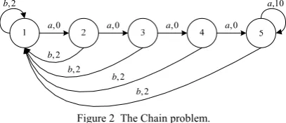
Chain problem, a classical benchmark platform for reinforcement learning which is widely applied, is shown in Fig. 2.

,0

a a,0

,0

a a,0

,10 a

, 2 b

, 2 b

, 2 b , 2

b , 2

b

Figure 2 The Chain problem.

dynamic system is known and the transition probability is unknown, and actions and states are independent.

In our experiments, we evaluate F-BRL using 500 simulations with 1000 steps in each simulation. We test the sample size K = 1000, and use the uniform prior to sample hypotheses. Table I shows the results of the total rewards and standard deviation. In this table, n.v. denotes not available, BEETLE [9] is the point-based value iteration algorithm which utilizes dynamic decision networks (DDNs) to factor states, and MC-BRL [12] is Monte Carlo Bayesian reinforcement learning algorithm,.

TABLEI

COMPARISON OF REWARDS AMONG DIFFERENT ALGORITHMS

PROBLEMS BEETLE MC-BRL F-BRL

CHAIN_TIED 3650±41 3618±29 3655±21 CHAIN _SEMI 3648±41 n.v. 3656±20 CHAIN _FULL 1754±42 1646±32 2279±21

Table I reports that F-BRL and BEETLE algorithm are closer to the true optimal value. However, in the larger CHAIN_FULL version, F-BRL has better performance than BEETLE. Because, we adopts the branch-and-bound pruning approach to prune the AND/OR tree of belief states online, this approach can effectively reduce the scale of problem. Therefore, F-BRL is able to achieve a better balance between exploration and exploitation than BEETLE.

TABLEII

COMPARISON OF COMPUTATION TIME AMONG DIFFERENT ALGORITHMS

PROBLEMS BEETLE MC-BRL F-BRL

CHAIN_TIED 1500 32 21 CHAIN _SEMI 1300 n.v. 30 CHAIN _FULL 18000 n.v. 98

Table II shows the computing time of different algorithms. We can see that F-BRL and MC-BRL take less online time than others. But, as shown in Table I, the accumulated rewards of MC-BRL are smaller than others; MC-BRL has greater errors. Offline method of F-BRL is the same as BEETLE. Nevertheless offline pre-computation does not affect real-time performance online. On the contrary, offline training could acquire better prior knowledge, and get as large as possible accumulate rewards. Therefore, F-BRL can better deal with the dilemma of exploration and exploitation in BRL.

B. RoboCupRescue Application

In order to verify the feasibility of F-BRL in real world application, we apply the proposed approach to the RoboCupRescue competition. In RoboCupRescue, the belief states space is very large. Taking a police agent as an example, the action set is A = {North; South; East; West; Clear}. A state can be described by approximately 1500 random variables, depending on the simulation [20, 27]: Roads: there are approximately 800 roads in a simulation and they can either be blocked or cleared. Consequently, there are 2800 _{possible configurations.}

Buildings: there are approximately 700 buildings in a

simulation and they can either be on fire or not. Therefore, there are 2700 _{possible configurations.}

Agentsposition: an agent can be on any of the 800 roads and there are usually 30 to 40 agents. In the worst case there are 80040 _possible

configurations. Consequently, the total number is |S| = 2800_×2700_×80040 _{in the worst case.}

The goal of RoboCupRescue is to reduce the earthquake damage as much as possible. The performance of the rescue agents is evaluated by considering the number of agents that are still alive, the healthiness of the survivors and the unburned area, which is formally defined by the following equation. As we can see, the most important aspect is the number of survivors. Therefore, agents should try to prioritize the task for rescuing civilians.

/

⎛ ⎞

=⎜_⎝ + S ⎟_⎠

V P B Bint

Sint (17)

where V is score, P is the number of living agents, S is the remaining number of health points of all agents, Sint is the total number of health points of all agents at the beginning, Bint is total buildings’ area at the beginning and B is the undestroyed area which is calculated using the fierceness value of all buildings.

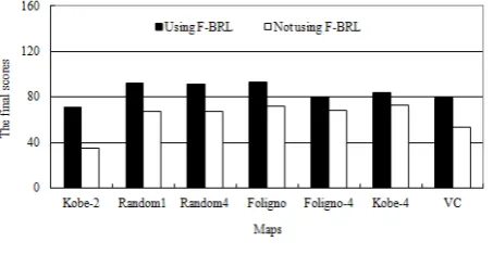
Figure 3 The final scores on 7 different maps

In RoboCupRescue, it was impossible to compare F-BRL with other POMDP algorithms. Therefore, to demonstrate the effectiveness of F-BRL, we compare the solution that uses F-BRL with that not using F-BRL. The baseline method which does not use F-BRL is the CSU_Yunlu RoboCuprescue framework which won the championship in China Open 2010. On the basis of this framework, we integrate F-BRL. The results obtained on 7 different maps are presented in Fig. 3. Each scenario was tested 10 times. From Fig. 3, we can conclude that F-BRL improves the performance of CSU_Yunlu RoboCupRescue team.

V. CONCLUSION

ACKNOWLEDGMENT

This work was supported by the NNSF of China under grant 61074058 and 60874042, and also was supported by the Shenzhen Technology Innovation Program of China under grant JCYJ20120617134831736.

REFERENCES

[1] K. Miyazaki, “Proposal of an Exploitation-oriented Learning Method on Multiple Rewards and Penalties Environments and the Design Guideline,” Journal of Computers, vol. 8, no. 7, pp. 1683-1690, Jul. 2013. [2] Z. Song, X. Chen, and S. Cong, “Agent Learning in

Relational Domains based on Logical MDP with Negation,” Journal of Computers, vol. 3, no. 9, pp. 29-38, Sep. 2008.

[3] Q. Zhang, M. Li, X. Wang, and Y. Zhang, "Reinforcement Learning in Robot Path Optimization," Journal of Software, vol. 7, no .3, pp. 657-662, Mar. 2012.

[4] H. Tang, W. Liu, W. Cheng, and L. Zhou, “Continuous-time MAXQ Algorithm for Web Service Composition,” Journal of Software, vol. 7, no. 5, pp. 943-950,May. 2012. [5] J. Yuan, X. Miao, L. Li L, and X. Jiang, “An Online Energy Saving Resource Optimization Methodology for Data Center,” Journal of Software, vol. 8, no. 8, pp. 1875-1880, Aug. 2013.

[6] H. Valizadegan, R. Jin, and S. Wang, “Learning to Trade Off Between Exploration and Exploitation in Multiclass Bandit Prediction,” In Proc KDD, 2011, pp. 204-212. [7] R. S. Sutton and A. G. Barto, “Reinforcement Learning:

An Introduction,” MIT Press, 1998, pp. 7-20.

[8] S. Ross, J. Pineau, B. Chaib-draa, and P. Kreitmann, “A Bayesian approach for learning and planning in partially observable Markov decision processes,” J Mach Learn Res, vol. 12, pp. 1729-1770, May. 2011.

[9] P. Poupart, N. Vlassis, J. Hoey, and R. Kevin, “An analytic solution to discrete Bayesian reinforcement learning,” In Proc. ICML, 2006, pp. 697-704.

[10] P. Poupart and N.A. Vlassis, “Model-based Bayesian Reinforcement Learning in Partially Observable Domains,” In Proc. ISAIM, 2008, pp. 1025-1032.

[11] S. Ross and J. Pineau, “Model-based Bayesian reinforcement learning in large structured domains,” In Proc. UAI, 2008, pp. 476-483.

[12] Y. Wang, K. S. Won, D. Hsu, and W. S. Lee, “Monte Carlo Bayesian reinforcement learning,” In Proc ICML, 2012, pp. 1135-1142.

[13] M. Duff, “Optimal learning: Computational procedures for Bayes-adaptive Markov decision processes,” Ph.D. dissertation, Dept. C.S, Univ. of Massassachusetts Amherst, Amherst, MA, 2002.

[14] X. Boyen and D. Koller, “Tractable inference for complex stochastic processes,” In Proc. UAI, 1998, pp. 33-42. [15] M. J. Kearns and D. Koller, “Efficient Reinforcement

Learning in Factored MDP,” In Proc IJCAI, 1999, pp. 740-747.

[16] C. Guestrin, D. Koller, R. Parr, and S. Venkataraman, “Efficient solution algorithms for factored MDP,” J Artif Intell Res, vol. 19, pp. 399–468, Oct. 2003.

[17] O. Kozloval, O. Sigaud, P. H. Wuillemin, and C. Meyer, “Considering unseen states as impossible in factored reinforcement learning,” In Proc ECML PKDD, 2009, pp. 721–735.

[18] N. Friedman and D. Koller, “Being Bayesian about network structure: a Bayesian approach to structure discovery in Bayesian networks,” Mach Learn, vol. 50, pp.

95-125, Jan. 2003.

[19] A. Kolobov and D. S. Weld, “Discovering hidden structure in factored MDP,” Artif Intell, vol. 189, pp. 19-47, Sep. 2012.

[20] S. Paquet, “Distributed decision-making and task coordination in dynamic uncertain and real-time multiagent environments” Ph.D. dissertation, Dept. C.S, Laval Univ., Québec, Canada, 2005.

[21] C. Boutilier, R. Dearden, and M. Goldszmidt, “Stochastic dynamic programming with factored representations,” Artif Intell, vol. 121, no. 1-2, pp. 49-107,Aug. 2000. [22] R. Jaulmes, J. Pineau, and D. Precup, “Active learning in

partially observable Markov decision processes,” In Proc ECML, 2005, pp. 601–608.

[23] M. Kearns, Y. Mansour, and A. Y. Ng, “A sparse sampling algorithm for near-optimal planning in large Markov decision processes,” Mach Learn, vol. 49, pp.193-208, Nov. 2002.

[24] T. Wang, D. Lizotte, M. Bowling, and D. Schuurmans, “Bayesian sparse sampling for online reward optimization,” In Proc ICML, 2005, pp. 956–963.

[25] C. Andrieu, A. Doucet, and R. Holenstein, “Particle Markov chain Monte Carlo methods,” J ROY STAT SOC B, vol. 72, no. 3, pp. 269–342, May. 2010.

[26] J. M. Porta, N. A. Vlassis, M. T. J. Spaaan, and P Poupart, “Point-based value iteration for continuous POMDP,” J Mach Learn Res, vol. 7, pp. 2329–2367, Nov. 2006. [27] B. Wu, H. Y. Zheng, and Y. P. Feng, “Point-based online

value iteration algorithm in large POMDP,” Appl Intell, vol. 39, no. 3, Aug. 2013.doi: 10.1007/s10489-013-0479-8 [28] J. Pineau, G. Gordon, and S. Thrun, “Anytime point-based approximations for large POMDP,” J. Artif Intell Res, vol. 27, pp. 335–380, Nov. 2006.

Bo Wu received the B.S., M.S., and Ph.D. degrees in computer science from the Central South University, Changsha, P.R. China, in 2000, 2003 and 2013 respectively. From 2003 to 2005, he was an Assistant Professor with Shenzhen polytechnic. From 2005 to 2009, he was a Lecturer with Shenzhen polytechnic. Since 2009, he has been an Associate Professor with the Education Technology and Information Center, Shenzhen polytechnic. His research interests include sequence decision-making, machine learning, and big data.

Yanpeng Feng received the B.S. and M.S. degrees in computer science and technology from the University of Science and Technology of China, Hefei, P. R. China, in 2003 and 2005 respectively. Since 2013, he was an Associate Research Fellow with the Education Technology and Information Center, Shenzhen polytechnic. His research interests include wireless sensor networks, intelligent decision, and big data.