Distributed Generation Placement Design and Contingency Analysis with Parallel Computing Technology

Distributed Generation Placement Design and

Contingency Analysis with Parallel Computing

Technology

Wenzhong Gao and Xi Chen

Tennessee Technological University, Electrical and Computing Engineering, Cookeville TN

Email:{wgao, xchen22}@tntech.edu

Abstract— Distributed Generation (DG) is a promising solution to many power system problems such as voltage regulation, power loss, etc. The location in the power system for DG placement is found to be very important. The additional DG placement strategy is also found to depend largely on the total capacity and location of DG already installed on the system. In this paper, a design strategy based on a proposed “critical bus tracking” method for Proton Exchange Membrane Fuel Cell (PEMFC) DG is tested on a modified IEEE 14 bus test case. Matlab Distributed Computing System (MDCS) is applied for a reduced computation time. Program for contingency analysis is also implemented in MDCS to test the design strategy. Tests are conducted in the modified IEEE 14 bus and 300 bus test cases to study the efficiency of the parallel algorithm for DG placement design and contingency analysis.

Index Terms— Distributed generation, distributed computing, contingency analysis, voltage stability, Proton Exchange Membrane Fuel Cell.

I. INTRODUCTION

Distributed generation (DG), including fuel cell, wind turbine, micro turbine, photo-voltaic (PV), wave etc, refers to small energy resources that generate electricity to support local loads. Compared to the traditional centralized power sources such as coal-fired power plants, nuclear reactors or hydropower, DG is often located near the load center (a city for example). DG has the advantage of greatly reduced or zero emission, and therefore, is suitable to be located near consumer’s sites. The reduced distance from the power source to the load center can in turn lead to lower power loss and better voltage regulation.

Among all the available DG technologies, fuel cell technology distinguishes itself with high potential in energy saving and emission reduction, as well as inherent fuel flexibility. Among different types of fuel cells, Proton Exchange Membrane Fuel Cell (PEMFC) is very attractive for DG application [1] with fast startup, simplicity of operation, zero emissions (when operating on hydrogen [H2]), although the performance of PEMFC is hindered by the low reaction temperature (60°C to

90°C [140°F to 194°F]).

The power loss in transmission lines is a big problem in electricity transmission. Although the voltage for power transmission over a long distance is raised to an extremely high value, a lot of power is still wasted in the transmission lines. The power loss on the transmission line is estimated to have been 7.2% in the USA in 1995. DG reduces power loss in an electric power system since it could be located near the load center and therefore the power transmission distance is reduced. Research has been conducted on the effects of reduced loss with placement of DG [2]. Different DG placement strategies have shown remarkable differences. In this paper, a PEMFC DG placement strategy based on “critical bus tracking” method is proposed. The proposed method looks for the “critical bus” where the effect of power loss reduction is the most dramatic as the total capacity of the PEMFC DG is gradually added to the system. Tests are conducted on a modified IEEE 14 bus test case [3] (See Appendix).

Different approaches in power system analysis, such as power flow, contingency analysis, PV curve and DG placement strategy are always quite time consuming. The computation time is a big concern especially for large power systems, which is generally the case. Meanwhile, distributed computing has proven to be successful in computation intensive areas such as weather forecast and atomic reaction simulations.

In this paper we developed a distributed computing algorithm for the proposed DG placement strategy to reduce the computer execution time. The code is implemented in Matlab Distributed Computing System (MDCS) of eight processors with a very satisfactory efficiency. More thorough comparison for different DG placement strategies is made possible with the increased computation speed.

this paper, a program for contingency analysis is implemented in MDCS. The program is then used to test the voltage stability of the power system with designed DG placement strategy. Tests are conducted on modified IEEE 14 bus and 300 bus test cases [3] (See Appendix). Excellent efficiency has been achieved for different cases. Thus, voltage stability contingency analysis process is greatly speeded up.

Figure 2. Matlab Distributed Computing System.

II. MATLABDISTRIBUTED COMPUTING SYSTEM

The Matlab Distributed Computing System (MDCS) enables distributed computing with Matlab codes. Independent Matlab operations therefore could be executed simultaneously on a cluster of computers [9].

In MDCS, a job is some large operation that needs to be performed in a Matlab session. A job is broken down into segments called tasks. The Matlab session in which the Matlab jobs and tasks are defined is called the client session. Often, this is on the machine where the Matlab code is programmed. The job manager is the part of the MDCS that coordinates the execution of jobs and the evaluation of their tasks. The job manager distributes the tasks for evaluation to the MDCS’s individual Matlab sessions called workers or labs. The system configuration is illustrated in Figure 1.

In this paper, the MDCS is working in Interactive Parallel Mode (pmode). The pmode of Matlab lets a client work interactively with parallel jobs running simultaneously on several labs. Commands at the pmode prompt are executed on all labs at the same time. Each lab executes the commands in its own workspace with its own variables. Communication among the workers and between a worker and the client is available after the computation has finished.

The MDCS used in this paper, as shown in Figure 2, is composed of four Dell Precision 390 PC’s with Inter CORE 2 DUO CPU of 2.4G/2.4G and 3.25GB of RAM. two workers are started in each PC. Therefore the number of maximum available workers is eight.

III. POWER FLOW ANALYSIS FOR DG

The power loss is a very important consideration factor in DG placement design. The power loss on the transmission line can be calculated by performing a power flow analysis. In this paper, the full Newton-Raphson’s method [10] is used in power flow analysis.

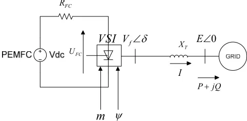
In power flow analysis, the PEMFC DG system interconnected to the power grid as shown in Figure 3 is modeled as a PV bus [11].

FC

R

FC

U

m

\

I T

X

G

‘

f

V E‘0

jQ

P

VSI

Figure 3. Equivalent circuit of grid-connected fuel cell DG system. MATLAB Client

Distributed Computing Toolbox

Job Manager

MATLAB Worker 1 MATLAB Distributed

Computing Engine

MATLAB Worker 2 MATLAB Distributed

Computing Engine

MATLAB Worker n MATLAB Distributed

Computing Engine

Figure 1. Configuration of Matlab Distributed Computing System.

The DG output voltage magnitude Vf is controlled by modulation index m of the voltage source inverter (VSI):

pu FC pu pu

f

m

u

V

_{. .} (1)

Through DG output voltage angel į, the active power delivered to grid is controlled by the power factor angle ȥ

of the VSI:

G

sin

T f

X

V

E

P

˜

(2)

T T

f

X E X

V E Q

2

cos

˜

G

(3)

»

»

¼

º

«

«

¬

ª

˜

\

G

tan

/

tan

1 ₂

P

X

E

P

T

(4)

and voltage magnitude Vf .

There is a limit on generated reactive power Q from the PEMFC DG system. When this limit is exceeded, the PEMFC DG system cannot generate more reactive power and the voltage magnitude is not controllable. In that case, the reactive power Q is fixed on the maximum value. Because the active power P is also fixed, the PEMFC DG could be now simulated as a PQ bus. In contrary with the load buses, the active load PL and reactive load QL will be negative in the DG system. There is also a lower limit of the generated reactive load bus Q. However, this limit is seldom exceeded in practical situations. The lower limit of the PEMFC DG system in this paper, therefore, is set to be zero.

IV. CONTINGENCY ANALYSIS

Contingency analysis in a power system area refers to the study of different situations where one or more of the system components, including a transmission line, generator, transformer, etc., are out of service either intentionally or due to fault. It is a “what-if” study. Contingency analysis is becoming a very important topic in power system analysis [4].

Accurate voltage stability contingency analysis could be accomplished by performing a PV (active load power-voltage magnitude) curve study [10]. Some other methods introducing different stability indices have also been introduced and compared in [12].

A line stability index LQP is proposed in [13]. The voltage stability index is derived from a 2 bus system without shunt capacitance as shown in Figure 4.

V1, V2 = voltage at the sending and receiving buses P1, Q1 = active and reactive power at the sending bus P2, Q2 = active and reactive power at the receiving bus S1, S2 = apparent power on the sending and receiving

buses

į = angle of the voltage at the receiving end

The current flow from bus 1 to bus 2 can be computed as:

jX

R

V

V

I

‘

‘

2

G

1

0

(5)

where R is the line resistance and X is the line reactance.

The received complex power at bus 2:

2 2 * 2

2

V

I

P

jQ

S

u

(6)

Plug in (5), we have:

° ° ¯ ° ° ® ­ » ¼ º « ¬ ª » ¼ º « ¬ ª 2 2 2 1 2 2 2 1 2 2 2 2 1 2 2 2 1 2 ) sin( ) cos (V ) sin( ) cos (V V X R R V X R X V Q V X R X V X R R V P G G G G (7)

If the line resistance is very small compared to the reactance, we have:

°

°

¯

°

°

®

­

2 1 2 2 2 2 1 2

cos

sin

V

V

V

XQ

V

V

XP

G

G

(8) Then: 1 cos

sin2 2

2 2 1 2 2 2 2 2 1 2 ¸ ¸ ¹ · ¨ ¨ © § ¸¸ ¹ · ¨¨ © § G G V V V XQ V V

XP ₍₉₎

So,

0 )

2

( _{2 1}2 ₂2 2 ₂2 ₂2 2

4

2 XQ V V X Q P X

V (10)

Consider (10) to be a quadratic equation of , for

to have a real solution, the discriminant must satisfy: 2 2

V

2 2

V

0 ) ( 4 ) 2

( 2 2

2 2 2 2 2 2 1

2V X Q P X t

XQ (11)

So, 2 2 2 2 1 2

4

V

_s

X

P

X

V

Q

d

(12)

Since the line is lossless, so

P

₁

P

₂ ,we have:

1

4

_{2 1}2 ₂

1 2 1

d

¸

¸

¹

·

¨

¨

©

§

¸

¸

¹

·

¨

¨

©

§

Q

P

V

X

V

X

(13) jX R 0 1‘

V V2‘G

1 1 1,Q,S

P

I

P2,Q2,S2

1

Bus Bus2

Figure 4. 2-bus model representation.

The line stability index is therefore defined for line between bus i and bus j as:

¸

¸

¹

·

¨

¨

©

§

¸

¸

¹

·

¨

¨

©

§

j i i i

ij

P

Q

V

X

V

X

LQP

4

_{2 2} 2 (14)

When there is no load at bus j, the LQP is 0. As the oad in the system increases, the LQP value increases from 0 to 1. The LQP value must be smaller than 1 for the system to be stable. The higher LQP value is, the closer the system is working near its stability margin. l

The system stability factor SLQP in a contingency is defined as the biggest LQPij value for all the transmission lines:

} max{LQP_ij

SLQP i,jall transmission lineindices

In case the system becomes unstable or collapses, Newton-Raphson’s method for power flow analysis will

converge. Therefore, the system stability factor cannot be calculated correctly by performing power flow analysis. In this case, the SLQP is assigned to be 1. not

Analysis results of SLQP as the active or reactive load increases on bus 4 of the IEEE 14 bus test case (shown in re 5 and 6) show very good relationship between the SLQP value and the system loads.

In this paper an (N-1) contingency analysis for line outage is applied. In one contingency, one transmission line is eliminated from the system.

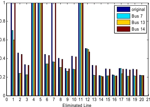
In case 2, a total 20 MW capacity of DG with available reactive power from zero to 20 MVar is assumed to have already been installed to bus 14. An additional 2MW PEMFC DG is then connected to each load bus respectively. The power loss reduction, shown in Figure 9, is most dramatic when the DG is connected to bus 7 or bus 13 (near 0.02 per unit, 2 MW). The power loss reduction on the previous “critical bus”-bus 14, however, is comparatively small (about 0.005 per unit, 0.5 MW).

V. DG PLACEMENTSTUDY

Studies have shown that DG has significant effects in power loss reduction, increased loadability, and improved voltage stability. However, the extent of such effects differs significantly for different placement strategies when same capacity of DG is installed to the system. In this section, two cases are studied for comparison of effects when a PEMFC DG is connected to the IEEE 14 bus test case.

In case 1, one PEMFC DG with an active power capacity of 2MW and available reactive power ranging from zero to 2MVar is available to connected to the load buses. The power loss reduction is calculated for different placements on the modified IEEE 14 bus test case. This DG is placed on each load bus (bus 4, bus 5, bus 7, bus 9, bus 10, bus 11, bus 12, bus 13, and bus 14) respectively. The power loss in the original system without DG is 39.30 MW. The total power loss reduction on all transmission lines compared to the original case, shown in Figure 7, is found to be most dramatic (about 0.011 per unit, 1.1 MW) when the DG is placed on bus 14. The load bus which resulst in the most power loss reduction when a DG with relatively small capacity is connected to it (Bus 14 in the modified IEEE 14 bus test case) is defined as the “critical bus” in this paper.

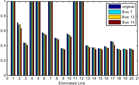
Line contingency analysis results with single line outages are shown in Figure 8. The system stability factor SLQP is calculated in the following four cases for each line outage contingency:

1.1. Original case. No DG is connected to the system;

0 0.5 1 1.5 2 2.5

0 0.1 0.2 0.3 0.4 0.5 0.6 0.7 0.8 0.9 1

S

ta

b

ilit

y

In

d

e

x

Additional Reactive Load on Bus 4

Figure 5. Change of SLQP as reactive load on bus 4 of the IEEE 14 bus test case increases.

1.2. The PEMFC DG is connected to bus 7; 1.3. The PEMFC DG is connected to bus 13; 1.4. The PEMFC DG is connected to bus 14;

The SLQP in case 1.4, where the PEMFC DG is connected to the “critical bus”-bus 14, attained the smallest SLQP value in all contingencies compared to other cases, which implies the highest system stability.

Contingency analysis results for line outage in Figure 10 also show most improvement to system stability when the DG is connected to bus 7 and 13, but further little improvement when connected to bus 14, compared to the original case with no DG connected. Therefore, the previous “critical bus” is no longer critical.

0 0.5 1 1.5 2 2.5 3

0 0.1 0.2 0.3 0.4 0.5 0.6 0.7 0.8 0.9 1

S

ta

b

ilit

y

I

n

d

e

x

Additional Ac tive Load on B us 4

Figure 6. Change of SLQP as active load on bus 4 of the IEEE 14 bus test case increases.

4 5 7 9 10 11 12 13 14

0 0.002 0.004 0.006 0.008 0.01 0.012

Load Buses

R

educ

ed

P

o

w

e

r Los

s

(

p

.u.)

Figure 7. Power loss reduction when a 2MW PEMFC DG is placed on each of the load bus respectively.

0 1 2 3 4 5 6 7 8 9 10 11 12 13 14 15 16 17 18 19 20 21 0

0.2 0.4 0.6 0.8 1

Eliminated Line

original Bus 7 Bus 13 Bus 14

VI. DG PLACEMENTSTRATEGY

Comparing results between Fig 7 and Fig 8, and between Figure 9 and Figure 10, we find out that: where the power loss reduction is smaller, the improvement for system stability is bigger. Therefore, power loss reduction is a good indication to judge a DG placement design.

Comparing results between Fig 7 and Fig 9, we find that the original “critical bus”, where the power loss reduction is the most dramatic when a DG is connected to it, may not be ‘critical’ after large amount of DG is already installed to it. Therefore, when a large capacity of DG units is available, it is not desirable to install all of them onto the same load bus. One explanation is that Bus 14 is farthest away from the swing. Therefore, transferring power from the swing bus to bus 14 results in the most dramatic power loss compared to other load buses. However, after a large amount of DG capacity is already installed to that bus, the originally “critical bus” becomes a power source and is able to support the load

itself without drawing power from the swing bus. In that case, the “critical bus” will not be “critical” anymore.

Based on the above analysis, a DG placement strategy based on “critical bus tracking” method for the modified IEEE 14 bus test case is proposed with the following assumptions:

4 5 7 9 10 11 12 13 14 0

0.005 0.01 0.015 0.02

Load Buses

R

educ

ed P

o

w

e

r Los

s

(

p

.u

.)

Figure 9. Power loss reduction when an additional 2MW PEMFC DG is placed on each of the load bus respectively (20MW DG is already connected to bus 14).

1. All the 9 load buses are assumed to be suitable for installation of PEMFC DG.

2. The total capacity of all the DGs installed at all buses is assumed to be 40 MW. The capacity of DG installed on each load bus is a multiple of 40KW. (i.e. each DG modular unit is rated at 40 KW).

3. The design that minimizes the total active power loss on the transmission line is considered the best design.

Steps of design:

1. Add a DG of 40 KW to each of the 9 load buses and calculate the power loss.

0 1 2 3 4 5 6 7 8 9 10 11 12 13 14 15 16 17 18 19 20 21 0

0.2 0.4 0.6 0.8 1

Eliminated Line

original Bus 7 Bus 1

2. Compare and find the critical bus that minimizes power loss when a DG of 40 KW is installed. 3. Add a DG of 40 KW to the critical bus.

Calculate the total capacity that has already been installed to the system. If all the 40MW is added: report the result. Otherwise: go to step 1.

The block diagram of the design process and the “critical bus tracking” method is shown in Figure 11 and Figure 12.

3 Bus 14

Input system data

Install 40KW DG to the critical bus

Update the system data

Cap=40MW? Total installed capacity: Cap=0

Report Results Critical bus tracking

No

Yes

Figure 11. DG placement design strategy block diagram for modified IEEE 14 bus test case.

0 1 2 3 4 5 6 7 8 9 10 11 12 13 14 15 16 17 18 19 20 21 0

0.2 0.4 0.6 0.8 1

Eliminated Line

original 40MW in bus 14 Proposed Method

Figure 13. Comparison of contingency analysis for: 1. Original case; No DG connected;

2. All 40MW capacity placed in the critical bus ‘14’;

3. 40MW capacity of DG connected with the proposed

“critical bus tracking” method. Add 40KW DG to bus i

Load bus number: i=1

Calculate and record line loss

Disconnect the DG on bus i

i=i+1;i>=9?

Compare the line loss; Find the critical bus Initial system data

Report critical bus No

Yes

Figure 12. Critical bus tracking method for modified IEEE 14 bus test case (sequential program).

The results of the proposed design strategy compared with a simple design strategy of connecting all the 40 MW capacity of DG to one single bus are shown in Table 1. In the second column of the table, a total capacity of 20.52 MW is installed on bus 14 while the remaining 19.48 MW is distributed among bus 4, bus 7, bus 10, and bus 13. The total power loss reduction is found to be 12.28 MW. In the third column, the power loss reduction when all the 40 MW capacity of DG is connected to the original “critical bus”-bus 14 is found to be 10.47 MW, which is almost 15% less than the proposed “critical bus tracking” DG placement strategy.

Contingency analysis results shown in Figure 13 also reflect better improvement for stability when the proposed method is compared with all 40 MW capacity placed in the original “critical bus”.

VII. PARALLELPROCESSING FOR DG PLACEMENT

STRATEGY AND CONTINGENCY ANALYSIS

The DG placement strategy has shown much more benefit to the power system compared with the simple method of connecting all the capacity to the “critical bus”. However, in the 14 bus test case, the time consumed for “critical bus tracking” is a considerable problem. The problem is more severe when the modified IEEE 300 bus test case is tested. Even the simple method of connecting all the capacity to the “critical bus” will take hours (most computation time is consumed in locating the “critical bus”). The time consumed for contingency analysis is also considerable. In this paper, we developed a parallel algorithm in MDCS to reduce the computation time.

In the parallel program for DG placement of IEEE 14 bus test case, the power loss reduction when 40 KW capacity of DG is added to each of the 9 load buses is calculated with parallel processing simultaneously, shown in Figure 14. The speed-up (Sequential code computation time / Parallel code computation time) is found to be 5.04 and the efficiency (Speed-up / number of processors) is found to be 63%. Shown in Table 2. The low efficiency is caused by the undesirable number of load buses (9) compared to the number of processers (8). Seven processors are left idle when the calculation for power loss reduction has finished for the first 8 load buses and only 1 more load bus is left. Figure 7 has shown that connecting a DG to bus 5 will result in the least amount of power loss reduction. In the modified parallel algorithm for DG placement of 14 bus test case, bus 5 is ignored. The speed-up is found to be 7.27 and efficiency to be 91%. Notice that shown in Table 1, no DG is connected to bus 5, therefore, the placement strategy remains the same for the modified code.

TABLE1 PERFORMANCE RESULTS FOR 14 BUSSYSTEM DG DESIGN “Critical Bus Tracking”

Strategy (MW)

Simple Strategy (All capacity installed on the

critical bus) (MW)

Bus 4 10.96 0

Bus 5 0 0

Bus 7 0.04 0

Bus 9 0 0

Bus 10 8.44 0

Bus 11 0 0

Bus12 0 0

Bus 13 0.04 0

Bus 14 20.52 40

Power loss

Add 40KW DG to bus i0 Load bus number: i0=i+0

Calculate and record line loss Disconnect the DG on bus i0

i=i+N;i>=9?

Compare the line loss; Find the critical bus Initial system data

Report critical bus Starting bus number i=1 N=number of processors

Add 40KW DG to bus i1 Load bus number: i1=i+1

Calculate and record line loss Disconnect the DG on bus i1

Add 40KW DG to bus iN Load bus number: iN=i+N-1

Calculate and record line loss Disconnect the DG on bus iN Distribute work

Gather results

No

Yes

Figure 14. Critical bus tracking method for modified IEEE 14 bus test case (parallel program).

1 2 3 4 5 6 7

S

peed U

p

2 4 6 886

88 90 92 94 96 98

Processors

E

ff

ici

e

n

cy %

Efficiency Speed up

Figure 16. Speed up and Efficiency vs. Number of processors of the MDCS when 16 load buses are considered for IEEE 300 bus case.

In Figure 15, we try to find the “critical bus” when only one 20 MW DG module is available to connect to the modified IEEE 300 bus test case. The efficiency and speedup as the number of load buses that are considered for DG unit placement increases is shown in Figure 15. The speed-up reached 7.7 and the efficiency reached 96% when more than 64 load buses are considered for DG unit placement.

In Figure 16, the speed-up and efficiency are shown when different numbers of processors are applied. The speedup increases from 1.6 to 6 as the efficiency decreases from 98% to 88% when the processors increase from 2 to 8.

In the parallel program for contingency analysis, each processor will take charge of equal number of line outage contingencies. The speed-up and efficiency are shown in Figure 17. The speedup is found to be 7.1 and efficiency to be 89% when more than 128 line outage contingencies are considered.

TABLE2 TIME CONSUMED FOR MODIFIED IEEE 14 BUS TEST CASE Time consumed

when 9 load buses considered (s)

Time consumed when 8 load buses

considered (s)

Sequential code 656.3 533.8

Parallel code 130.3 73.4

Speed up 5.04 7.27

Efficiency 63% 91%

5.2 5.6 6 6.4 6.8 7.2

S

pee

d U

p

8 16 32 64 128 4110.65

0.7 0.75 0.8 0.85 0.9

Number of Contingencies Considered

E

ff

ici

e

n

cy

%

Figure 17. Speed up and Efficiency vs. Number of Contingencies considered for IEEE 300 bus test case.

8 16 32 64 231

5.6 6 6.4 6.8 7.2 7.6 8

Number of Load Buses Considered

S

peed U

p

70 75 80 85 90 95 100

Ef

fi

ci

e

n

cy %

Figure 15. Speed up and Efficiency vs. Number of considered load buses for DG placement of IEEE 300 bus test case.

VIII.CONCLUSION

DG has proven to be able to reduce the power loss and increase the system stability. The extent of such effects is greatly influenced by the location where the DG is connected. The location of the “critical bus”, where the effects of power loss reduction are most dramatic among all the load buses, is also found to vary as the total capacity and location of DG already installed on the system varies. Therefore, a careful design of the DG placement strategy will achieve the most improvement to the power system performance with limited total DG capacity.

method.

Parallel codes have been implemented in MDCS for DG placement design and line outage contingency analysis. The computation time for optimal DG placement design and contingency analysis has been greatly reduced. Parallel processing has proven to be a desirable tool for DG placement design and its performance analysis.

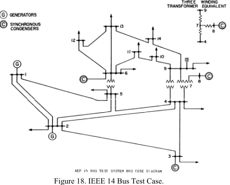
APPENDIX

Modified IEEE 14 bus test case [3]:

The diagram of IEEE 14 Bus Test Case with a rated power of 100MW is shown in Figure 18. The system is composed of 1 slack bus (bus 1), 1 generator (bus 2), 3 synchronous condensers (bus 3, 6, and 8), and 9 load buses. There are totally 20 transmission lines. The shunt susceptance is ignored. The load on all the buses is increased by 150% to stress the system.

Modified IEEE 300 bus test case [3]:

The diagram of IEEE 300 Bus Test Case is composed of 1 slack bus, 231 load buses and 68 generation buses with a total of 411 transmission lines. The rated power is 100 MW. Shunt susceptance is also not considered in this paper.

REFERENCES

[1] S. Lasher, R. Zogg, E. Carlson, P. Couch, M. Hooks, K. Roth, J. Brodrick, “PEM Fuel Cells For Distributed Generation,” American Society of Heating, Refrigerating and Air-Conditioning Engineers Journal, Vol. 48, November 2006.

[2] T. Griffin, K. Tomsovic, D. Secrest, A. Law, “Placement of dispersed generation systems for reduced losses,” Proceedings of the 33rd Annual Hawaii international Conference, pp.1-9, Jan 4-7 2000.

[3] R. Christie, UW Power System Test Case Archive, Available: http://www.ee.washington.edu/research/pstca/.

[4] “Using the Contingency Analysis in Power World,” Available: http://ecow.engr.wisc.edu/cgibin/get/ece/427/hiskens/1discussion/ pwcontingencyanalysis.pdf.

[5] S. Repo, P. Jarentausta, “Contingency analysis for a large number of voltage stability studies,” PowerTech Budapest 99 International Conference on Electric Power Engineering, 29 Aug. - 2 Sept. 1999, pp. 34.

[6] C. N. Lu, M. Unum, “Interactive simulation of branch outages with remedial action on a personal computer for the study of

security analysis,” IEEE Transaction on Power Systems, Vol. 6, Aug. 1991, pp. 1266 – 1271.

[7] R. H. Chen, J. Gao, O. P. Malik, G. S. Hope, S. Wang, N. Xiang, “Multi-contingency preprocessing for security assessment using physical concepts and CQR with classifications,” IEEE Transaction on Power Systems, Vol. 8, Aug. 1993 pp.840 – 848. [8] P. A. Ruiz, P. W. Sauer, “Voltage and Reactive Power Estimation

for Contingency Analysis Using Sensitivities,” IEEE Transaction on Power Systems, Vol. 22, pp. 639 – 647, May 2007.

[9] “Distributed Computing Toolbox User's Guide,” Available: http://www.mathworks.com/access/helpdesk/help/toolbox/distcom p/index.html?/access/helpdesk/help/toolbox/distcomp/bqqaxq0.ht ml&http://www.mathworks.com/access/helpdesk/help/toolbox/dist comp/distcomp_product_page.html.

[10] Mariesa Crow, Computational Methods for Electric Power Systems, CRC Press, 2003.

[11] H. Chen, J. Chen, D. Shi, X. Duan, “Power Flow Study and Voltage Stability Analysis for Distribution Systems with Distributed Generation,” IEEE Power Engineering Society General Meeting, pp.1-8, 18-22 June 2006.

[12] C. Reis, F. P. M. Barbosa, “A Comparison of Voltage Stability Indices,” Electrotechnical Conference, pp. 1007 – 1010, 2006. [13] A. Mohamed, G. B. Jasmon, S. Yusoff, “A Static Voltage Collapse

Indicator using Line Stability Factors,” Journal of Industrial Technology, Vol. 7, No. 1, pp. 73-85, 1989.

Figure 18. IEEE 14 Bus Test Case.

David Wenzhong Gao received the B.S. degree in Aeronautical Propulsion Control Engineering from Northwestern Polytechnic University, Xi’an, China; his M.S. degree and Ph.D. degree in Electrical and Computer Engineering specializing in electric power engineering from Georgia Institute of Technology, Atlanta, USA. Currently, he works as an Assistant Professor in Tennessee Tech University. His research interests include renewable energy, alternative power systems, hybrid electric propulsion systems, power system modeling and simulation, and electric machinery and drive.