Research Article
Feedforward and Feedback Control Performance Assessment for
Nonlinear Systems
Zhiguo Wang and Jun Chen
Key Laboratory of Advanced Process Control for Light Industry (Ministry of Education), Institute of Automation, Jiangnan University, Wux 214122, China
Correspondence should be addressed to Zhiguo Wang; jndx [email protected]
Received 23 January 2014; Revised 29 March 2014; Accepted 30 March 2014; Published 24 April 2014 Academic Editor: Shuping He
Copyright © 2014 Z. Wang and J. Chen. This is an open access article distributed under the Creative Commons Attribution License, which permits unrestricted use, distribution, and reproduction in any medium, provided the original work is properly cited. A performance assessment method for nonlinear feedforward and feedback control systems is proposed in this paper. First, the existence of minimum variance performance bound for two nonlinear systems with different structures is analyzed, and the closed-loop model of nonlinear system is obtained with the help of iterative orthogonal least squares identification method. Then, the technology of variance analysis is introduced to establish the variance contributions due to both disturbances and controller. A nonlinear performance index for the feedforward and feedback control systems is estimated using an ANOVA-like variance decomposition method. Finally, a meaningful example is simulated to show the effectiveness of our method.
1. Introduction
The technology of control performance assessment (CPA) has attracted much attention in recent years, due to the extensive application of automatic control systems in indus-trial area. CPA is a management tool to maintain efficient operation performance of automation systems. The main aim is to evaluate the performance of control loops in control systems, diagnose the reason of poor performance, and present effective proposals for improvement once the control performance of a running controller cannot meet the desired requirements.
The study of CPA began to blossom some 20 years ago with the pioneering work by Harris [1]; he proposed a linear performance index based on minimum variance benchmark. Desborough and Harris [2] proposed a nor-malized performance index for assessment of linear SISO controller performance, which can be estimated by linear regression methods. Stanfelj et al. [3] presented a method that utilized autocorrelation and cross correlation functions for monitoring and diagnosing the cause of poor performance of feedforward and feedback control systems. Desborough and Harris [4] developed a performance assessment algo-rithm based on variance table to investigate the variance contributions due to disturbances and controllers for a linear
feedforward and feedback system. Harris et al. [5] developed a method for assessing the performance of linear MIMO control systems, and this method requires an estimate of the process interactor matrix that characterizes the dead-time structure. Almost at the same time, Huang et al. [6] developed a new approach based on filtering and correlation (FCOR) analysis of the process output and filtered data, which can be used to estimate the controller performance of a general class of linear MIMO processes. Subsequently, Huang et al. [7] developed a method for the performance assessment of linear multivariate feedback plus feedforward control systems using minimum variance control as the benchmark. CPA theoretical issues have been reported by several literatures, such as the references published by Qin [8], Huang and Shah [9], and Jelali [10].
Although the field of CPA has received much attention in theory and engineering in recent years [11–14], the most previous studies are focused on linear systems. In real applications, the industrial processes are naturally nonlinear systems. The estimation of the minimum variance perfor-mance lower bound (MVPLB) and the perforperfor-mance index using the linear control performance assessment techniques may be distorted by these nonlinearities. Due to the internal complexity and lack of effective mathematical tools, far less
Volume 2014, Article ID 597805, 12 pages http://dx.doi.org/10.1155/2014/597805
has been written on the CPA methods for nonlinear systems. For a special class of nonlinear SISO processes that can be described by the superposition of a nonlinear dynamic model and additive linear disturbance, Harris and Yu [15] presented a method to estimate the MVPLB using closed-loop data. Continuing this idea, estimates of the MVPLB for the moderate valve stiction cases are proposed by Yu et al. [16]. Yu et al. [17] proposed a new CPA performance index for general nonlinear SISO models based on an ANOVA-like variance decomposition method. This new performance index is not based on the MVPLB, but it can be used to estimate the MVPLB for some nonlinear systems detailed are discussed in [15]. Considering the process nonlinearity and valve stiction nonlinearity in control system, Zhang [18] proposed some CPA methods for nonlinear systems based on minimum variance benchmark. Yu et al. [19] extended CPA to nonlinear MIMO systems. However, in order to make the problem tractable, they restrict the system structure to be a model with additive linear disturbances and where the nonlinearity is in the form of valve stiction.
In spite of the fact that multivariate control schemes are justified from an economic and quality improvement stand-point, the univariate controllers are the mostly used con-trollers in practical applications. The performance of these SISO control schemes can be enhanced by including feed-forward elements. In this paper, we study the performance assessment for nonlinear feedforward and feedback control systems. The objective of our work is to estimate the MVPLB for this nonlinear system and analyze the contribution of each controller for the overall performance bound. This study has an important guiding significance for the adjustment and design of the actual control system. Two common situations are often encountered in pragmatic feedforward and feedback control systems. The first case is, although a feedforward variable can be measured, it is not used in the control systems; in such situation, the result of CPA for nonlinear feedforward and feedback control systems can provide an estimation of the variance reductions if feedforward controller is considered. In the other case, a feedforward variable is both measured and used in a feedforward and feedback control scheme, and then, the performance of the individual controllers can be assessed by the result of this paper, such that we can determine which controller should be principally adjusted to improve the performance of feedforward and feedback control systems.
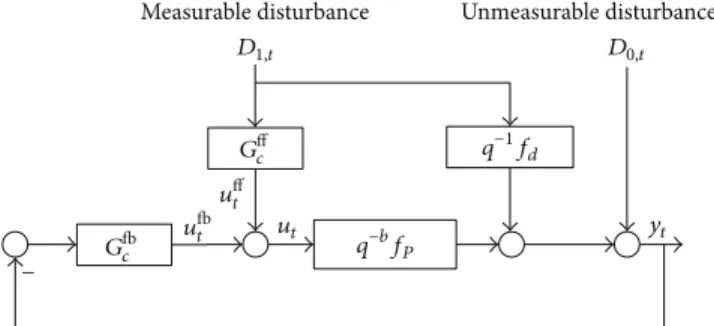
Based on some methods for the performance assessment of linear feedforward and feedback control systems, this paper is an extension to nonlinear systems. The outline of this paper is organized as follows. As a prerequisite, the performance assessment of linear feedforward and feedback systems is discussed inSection 2. InSection 3, the existence of MVPLB for nonlinear feedforward and feedback systems is analyzed. InSection 4, a description of the ANOVA-like vari-ance decomposition method is given and a new performvari-ance index of nonlinear control systems is proposed. Finally, a simulation is made to illustrate the proposed method-ology in Section 5, and this is followed by a conclusion inSection 6. Unmeasurable disturbance Measurable disturbance − D0,t q−1fd ut q−bfP yt D1,t Gffc Gfbc u fb t ufft
Figure 1: Schematic of feedforward and feedback control system.
2. Analysis of Variance in Linear Feedforward
and Feedback Control System
A structural schematic of general feedforward and feedback control system is given inFigure 1, where𝑦𝑡is output variable of the process,𝑢𝑡is manipulated variable which is adjusted by summing the outputs from the feedback controller𝑢𝑡fb and feedforward controller𝑢ff𝑓.𝐺fb𝑐 is feedback controller transfer function, and𝐺ff𝑐 is feedforward controller transfer function. 𝑞−𝑏𝑓𝑃 represents the process model that may be linear or
nonlinear.𝑏is the number of whole periods of process delay. 𝑞−𝑙𝑓𝑑𝐷1,𝑡represents the effect that the measured disturbance
𝐷1,𝑡has on the process output, and𝑙is the number of periods
of delay it takes for a change in 𝐷1,𝑡 to begin to affect the output. In linear systems, 𝑞−𝑙𝑓𝑑𝐷1,𝑡 is often expressed by transfer function as 𝑞−𝑙𝑁𝑑𝐷1,𝑡. 𝐷0,𝑡 and 𝐷1,𝑡 represent the unmeasured and measured disturbances, respectively. In this paper, work is based on the assumption that there is no cross correlation among the unmeasured and measured disturbances, and this is reasonable for many industrial processes.
In linear systems, the delay-free process model𝑓𝑃can be represented by the following equation:
𝑓𝑃= 𝜔 (𝑞
−1)
𝛿 (𝑞−1), (1)
where𝜔(𝑞−1)and𝛿(𝑞−1)are stable polynomials in the back-shift operator𝑞−1. Disturbances𝐷0,𝑡and𝐷1,𝑡are represented by autoregressive integrated moving average (ARIMA) time series models:
𝐷𝑖,𝑡= 𝜃𝑖(𝑞
−1)
𝜑𝑖(𝑞−1) ∇𝑑𝑖𝛼𝑖,𝑡, 𝑖 = 0, 1. (2)
{𝛼𝑖,𝑡} is a sequence of independently and identically dis-tributed random variables with mean zero and constant variance𝜎2𝑖.𝜃𝑖(𝑞−1)and𝜑𝑖(𝑞−1)are monic and stable poly-nomials. The difference operator is defined as∇def= (1 − 𝑞−1), and𝑑𝑖 is the degree of differencing. The linear feedforward
and feedback control system can be modeled as the sum of two disturbances and a linear transfer function:
𝑦𝑡= 𝑞−𝑏𝜔 (𝑞
−1)
𝛿 (𝑞−1)𝑢𝑡+ 𝐷0,𝑡+ 𝑞−𝑙𝑁𝑑𝐷1,𝑡. (3)
Substituting the feedforward and feedback controller repre-sentation into above equation and multiplying both sides by 𝑞𝑑and collecting terms
𝑦𝑡+𝑏= 𝜔 (𝑞−1) 𝛿 (𝑞−1)𝑢 fb 𝑡 + 𝐷0,𝑡+𝑏+ 𝜔 (𝑞−1) 𝛿 (𝑞−1)𝑢 ff 𝑡 + 𝑞−𝑙𝑁𝑑𝐷1,𝑡+𝑏. (4) In an analogous manner to the minimum variance feedback controller, the design of minimum variance feedforward and feedback controller can be derived. The research result of Desborough and Harris [4] reported that the linear closed-loop system can be described in terms of the unmeasured disturbance driving force and the measured feedforward variable. We do the similar work, which yields
𝑦𝑡+𝑏= 𝜔 (𝑞 −1) 𝛿 (𝑞−1) (−𝐺 fb 𝑐𝑦𝑡) + 𝜃0(𝑞−1) 𝜑0(𝑞−1) ∇𝑑0𝛼0,𝑡+𝑏 +𝜔 (𝑞 −1) 𝛿 (𝑞−1)𝐺 ff 𝑐𝐷1,𝑡+ 𝑞−𝑙𝑁𝑑𝐷1,𝑡+𝑏 = 𝜃0(𝑞 −1) /𝜑 0(𝑞−1) ∇𝑑0 1 + 𝑞−𝑏[𝜔 (𝑞−1) /𝛿 (𝑞−1)] 𝐺fb 𝑐 𝛼0,𝑡+𝑏 + 𝑞 −𝑏𝐺 𝑃(𝑞−1) 𝐺ff𝑐 + 𝑞−𝑙𝑁𝑑 1 + 𝑞−𝑏[𝜔 (𝑞−1) /𝛿 (𝑞−1)] 𝐺fb 𝑐 𝐷1,𝑡+𝑏 = 𝜓0(𝑞−1) 𝛼0,𝑡+𝑏+ 𝜓1(𝑞−1) 𝐷1,𝑡+𝑏, (5)
where𝜓0(𝑞−1)is the closed-loop transfer function between 𝑦𝑡 and the driving force for the unmeasured disturbance. 𝜓1(𝑞−1) is the closed-loop transfer function between 𝑦
𝑡
and measured feedforward variable𝐷1,𝑡. Alternatively, the process can be described in terms of the driving forces alone: 𝑦𝑡= 𝜓0(𝑞−1) 𝛼0,𝑡+𝑏+ 𝜓1(𝑞−1) 𝛼1,𝑡+𝑏. (6)
Each of the closed-loop transfer functions in (6) can be expanded in a convergent power series in𝑞−1:
𝜓𝑖(𝑞−1) =∑∞
ℎ=0
𝜓𝑖,ℎ𝑞−ℎ. (7)
This expansion is obtained by writing each transfer function as a ratio of polynomials𝑞−1and then dividing the numerator into the denominator using polynomial long division. Then the process output can be extended as
𝑦𝑡+𝑏= 𝑦0,𝑡+𝑏+ 𝑦1,𝑡+𝑏=∑∞ ℎ=0 𝜓0,ℎ𝑞−ℎ𝛼0,𝑡+𝑏+∑∞ ℎ=0 𝜓1,ℎ𝑞−ℎ𝛼1,𝑡+𝑏. (8)
The term 𝑦0,𝑡+𝑏 is the contribution of unmeasured distur-bance𝐷0,𝑡to the process output; it can be written as
𝑦0,𝑡+𝑏= (1 + 𝜓0,1𝑞−1+ ⋅ ⋅ ⋅ + 𝜓0,𝑏−1𝑞−(𝑏−1)) 𝛼0,𝑡+𝑏 + (𝜓0,𝑏𝑞−𝑏+ 𝜓 0,𝑏+1𝑞−(𝑏+1)+ ⋅ ⋅ ⋅ ) 𝛼1,𝑡+𝑏 = 𝑒0,𝑡+𝑏/𝑡+∑∞ ℎ=𝑏 𝜓0,ℎ𝑞−ℎ𝛼0,𝑡+𝑏= 𝑒0,𝑡+𝑏/𝑡+ 𝑦fb 0,𝑡+𝑏. (9)
The first term 𝑒0,𝑡+𝑏/𝑡 in above function is recognized as the prediction error, which is independent of the second term. The second term is the contribution to the process output 𝑦0,𝑡+𝑏 which arises from the nonoptimality of the control associated with the unmeasured disturbance, and it is also a function of the process dynamics, the unmeasured disturbance, and the feedback controller only.
In a similar manner, the contribution of the measured disturbance𝐷1,𝑡to the process output can be written as
𝑦1,𝑡+𝑏= 𝑒1,𝑡+𝑏/𝑡+ (𝜓1,𝑏𝑞−𝑏+ ⋅ ⋅ ⋅ + 𝜓1,𝑏+𝑙−1𝑞−(𝑏+𝑙−1)) 𝛼1,𝑡+𝑏 + (𝜓1,𝑏+𝑙𝑞−(𝑏+𝑙)+ 𝜓 1,𝑏+𝑙+1𝑞−(𝑏+𝑙+1)+ ⋅ ⋅ ⋅ ) 𝛼1,𝑡+𝑏 = 𝑒1,𝑡+𝑏/𝑡+ 𝑏+𝑙−1 ∑ ℎ=𝑏 𝜓1,ℎ𝑞−ℎ𝛼1,𝑡+𝑏 + ∑∞ ℎ=𝑏+𝑙 𝜓1,ℎ𝑞−ℎ𝛼1,𝑡+𝑏= 𝑒1,𝑡+𝑏/𝑡+ 𝑦ff 1,𝑡+𝑏+ 𝑦1,𝑡+𝑏ff&fb, (10) where 𝑒1,𝑡+𝑏/𝑡 = { { { { { { { { { { { { { { { { { 0, 𝑙 ≥ 𝑏 (𝜓⏟⏟⏟⏟⏟⏟⏟⏟⏟⏟⏟⏟⏟⏟⏟⏟⏟⏟⏟⏟⏟⏟⏟⏟⏟⏟⏟⏟⏟⏟⏟⏟⏟⏟⏟⏟⏟⏟⏟⏟⏟⏟⏟⏟⏟⏟⏟1,0𝑞0+ ⋅ ⋅ ⋅ + 𝜓1,𝑙−1𝑞−(𝑙−1) 0 + 𝜓1,𝑙𝑞−𝑙 + 𝜓1,𝑙+1𝑞−(𝑙+1)+ ⋅ ⋅ ⋅ + 𝜓 1,𝑏−1𝑞−(𝑏−1)) 𝛼1,𝑡+𝑏 𝑙 < 𝑏. (11) In (10), the first term𝑒1,𝑡+𝑏/𝑡 is the prediction error for the measured disturbance, and it is independent of the second and third terms. The second term is the contribution to the output 𝑦1,𝑡+𝑏 which arises from the nonoptimality of the feedforward controller only, and the third term is the contribution which arises from the combined effect of the nonoptimality of the feedforward controller and the feedback controller.
Since it has been assumed that the measured and unmea-sured disturbances are not cross correlated, the prediction error 𝑒0,𝑡+𝑏/𝑡 and 𝑒1,𝑡+𝑏−𝑙/𝑡 are independent of all the con-trollers. Then, the process output under minimum variance control is given by the sum of the individual error in forecasting the effect of the disturbances:
𝑦mv
𝑡+𝑏= 𝑒0,𝑡+𝑏/𝑡+ 𝑒1,𝑡+𝑏−𝑙/𝑡, (12)
and the MVPLB can be written as
3. MVPLB of Nonlinear Feedforward and
Feedback Control System
Due to the effect of various factors such as complexity of nonlinear behavior and challenges in model determination and parameter estimation, far less has been written to extend the methods for performance assessment to nonlinear systems. In order to simplify the analysis and without loss of generality, the problem of estimation for minimum variance performance bound for nonlinear feedforward and feedback systems is given in two aspects.
First, we only assume that the process model has a nonlinear representation in the structural schematicFigure 1, and this is not very restrictive in many applications. Then, the closed output𝑏-steps into the future of the nonlinear system can be expressed as
𝑦𝑡+𝑏= 𝑓𝑃(𝑢∗𝑡) + 𝐷0,𝑡+𝑏+ 𝑁𝑑𝐷1,𝑡+𝑏−𝑙, (14)
where the notation 𝑓𝑃(⋅) denotes a nonlinear function of process model, and the superscript ∗ is used to represent the vector collecting the immediate historical values; that is, 𝑢∗𝑡 def= (𝑢𝑡−1, . . . , 𝑢𝑡−𝑛𝑢). Decomposing the unmeasured disturbance𝐷0,𝑡+𝑏into a prediction error and a prediction
𝐷0,𝑡+𝑏= 𝑒0,𝑡+𝑏/𝑡+ ̂𝐷0,𝑡+𝑏/𝑡, (15)
the prediction𝐷̂0,𝑡+𝑏/𝑡 is the𝑏-step ahead minimum mean square error prediction for the value of the unmeasured dis-turbance𝑏steps into the future. The effects of the measured feedforward variables are also decomposed into a prediction error and a prediction
𝑁𝑑𝐷1,𝑡+𝑏−𝑙= 𝑒1,𝑡+𝑏−𝑙/𝑡+ ̂𝐷1,𝑡+𝑏−𝑙/𝑡. (16)
The prediction𝐷̂1,𝑡+𝑏−𝑙/𝑡 is the𝑏 − 𝑙 step ahead minimum mean square error prediction for the value of the measured disturbance𝑏 − 𝑙steps into the future. Note that if𝑙is greater than or equal to𝑏, then𝑒1,𝑡+𝑏−𝑙/𝑡 = 0. This implies that there is no prediction error since we exactly know the future value of the effect on the process of the measured disturbance.
The minimum variance control law is found by minimiz-ing the mean square error of the output:
𝑦𝑡+𝑏= 𝑓𝑃(𝑢∗𝑡) + 𝐷0,𝑡+𝑏+ 𝑁𝑑𝐷1,𝑡+𝑏−𝑙 = 𝑓𝑃(𝑢∗𝑡) + 𝑒0,𝑡+𝑏/𝑡+ ̂𝐷0,𝑡+𝑏/𝑡+ 𝑒1,𝑡+𝑏−𝑙/𝑡+ ̂𝐷1,𝑡+𝑏−𝑙/𝑡 = 𝑒⏟⏟⏟⏟⏟⏟⏟⏟⏟⏟⏟⏟⏟⏟⏟⏟⏟⏟⏟⏟⏟⏟⏟⏟⏟⏟⏟⏟⏟⏟⏟0,𝑡+𝑏/𝑡+ 𝑒1,𝑡+𝑏−𝑙/𝑡 term1 + 𝑓⏟⏟⏟⏟⏟⏟⏟⏟⏟⏟⏟⏟⏟⏟⏟⏟⏟⏟⏟⏟⏟⏟⏟⏟⏟⏟⏟⏟⏟⏟⏟⏟⏟⏟⏟⏟⏟⏟⏟⏟⏟⏟⏟⏟⏟⏟⏟⏟⏟⏟⏟⏟⏟𝑃(𝑢∗𝑡) + ̂𝐷0,𝑡+𝑏/𝑡+ ̂𝐷1,𝑡+𝑏−𝑙/𝑡 term2 . (17)
It follows from this formula that the minimum variance controller (MVC) set the manipulated variables to exactly cancel the predictions; that is,
𝑓𝑃(𝑢fb
𝑡 , 𝑢𝑡ff) + ̂𝐷0,𝑡+𝑏/𝑡+ ̂𝐷1,𝑡+𝑏−𝑙/𝑡= 0. (18)
Then the process output under this control scheme can be denoted by 𝑦mv 𝑡+𝑏= 𝑒0,𝑡+𝑏/𝑡+ { { { 0, 𝑙 ≥ 𝑏 𝑒1,𝑡+𝑏−𝑙/𝑡, 𝑙 < 𝑏. (19)
As we have assumed that there is no cross correlation among the unmeasured and measured disturbances, the prediction errors 𝑒0,𝑡+𝑏/𝑡 and 𝑒1,𝑡+𝑏−𝑙/𝑡 are independent and unrelated with controller parameters. Then, the MVPLB of closed-loop output is 𝜎mv2 =var(𝑒0,𝑡+𝑏/𝑡) +var(𝑒1,𝑡+𝑏−𝑙/𝑡) = (1 + 𝜓20,1+ ⋅ ⋅ ⋅ + 𝜓0,𝑏−12 ) 𝜎02 +{{ { 0 𝑙 ≥ 𝑏 (𝜓2 1,0+ 𝜓1,12 + ⋅ ⋅ ⋅ + 𝜓1,𝑏−𝑙−12 ) 𝜎12 𝑙 < 𝑏. (20)
From above derivation, we can conclude that the MVPLB of nonlinear feedforward and feedback system is identical to that of linear system. The difference is that it is possible to adopt different controllers for obtaining same minimum variance.
Second, a more general form of nonlinear feedforward and feedback control systems is considered:
𝑦𝑡= 𝑞⏟⏟⏟⏟⏟⏟⏟⏟⏟⏟⏟⏟⏟⏟⏟⏟⏟−𝑏𝑓𝑃(𝑢∗𝑡) nonlinear + ̃𝐷⏟⏟⏟⏟⏟⏟⏟0,𝑡 nonlinear + ̃𝐷⏟⏟⏟⏟⏟⏟⏟⏟⏟1,𝑡−𝑙 nonlinear , (21)
where the terms𝐷̃0,𝑡and𝐷̃1,𝑡−𝑙are called output disturbances which represent the effect that the unmeasured and measured disturbances have on the process output, respectively. They are also nonlinear and can be represented by nonlinear ARMA model as ̃ 𝐷0,𝑡= 𝑓0,𝐷(̃𝐷∗0,𝑡−1, 𝛼0,𝑡−1∗ ) + 𝛼0,𝑡, ̃ 𝐷1,𝑡= 𝑓𝑑𝐷1,𝑡= 𝑓1,𝐷(̃𝐷∗ 1,𝑡−1, 𝛼1,𝑡−1∗ ) + 𝛼1,𝑡. (22)
Further, we assume that the output disturbance admits a representation of the form
𝛾𝑖(𝑞−1) ∇𝑑𝑖𝐷̃ 𝑖,𝑡= 𝑚 ∑ 𝑘=1 𝜃𝑖,𝑘𝛼𝑖,𝑡−𝑘+ ∑𝑚 𝑘1=1 𝑚 ∑ 𝑘2=𝑘1 𝜃𝑖,𝑘1𝑘2𝛼𝑖,𝑡−𝑘1𝛼𝑡−𝑘2+ ⋅ ⋅ ⋅ + ∑𝑚 𝑘1=1 ⋅ ⋅ ⋅ ∑𝑚 𝑘𝑘=𝑘𝑘−1 𝜃𝑖,𝑘1⋅⋅⋅𝑘𝑘𝛼𝑖,𝑡−𝑘1⋅ ⋅ ⋅ 𝛼𝑖,𝑡−𝑘𝑘 ⏟⏟⏟⏟⏟⏟⏟⏟⏟⏟⏟⏟⏟⏟⏟⏟⏟⏟⏟⏟⏟⏟⏟⏟⏟⏟⏟⏟⏟⏟⏟⏟⏟⏟⏟⏟⏟⏟⏟⏟⏟⏟⏟⏟⏟⏟⏟⏟⏟⏟⏟⏟⏟⏟⏟⏟⏟⏟⏟⏟⏟⏟⏟⏟⏟⏟⏟⏟⏟⏟⏟⏟⏟⏟⏟⏟⏟⏟⏟⏟⏟⏟⏟⏟⏟⏟⏟⏟⏟⏟⏟⏟⏟⏟⏟⏟⏟⏟⏟⏟⏟⏟⏟⏟⏟⏟⏟⏟⏟⏟⏟⏟⏟⏟⏟⏟⏟⏟⏟⏟⏟⏟⏟⏟⏟⏟⏟⏟⏟⏟⏟⏟⏟⏟⏟⏟⏟⏟⏟⏟⏟⏟⏟⏟⏟⏟⏟⏟⏟⏟⏟⏟⏟⏟⏟ 𝑓𝑖,𝐷(𝛼∗𝑖,𝑡−1) + 𝛼𝑖,𝑡, (23)
where {𝛼𝑖,𝑡} is a white noise sequence with mean 𝜇𝑖,𝛼 and variance 𝜎𝑖,𝛼2 , and 𝛾𝑖(𝑞−1) is monic and stable polynomial, and we also assume that the disturbance model is invertible. Multiply both sides by𝑞𝑏and substitute for all values of𝑦𝑡+𝑏−𝑖, 𝑖 = 1, . . . , 𝑏 − 1, in (21): 𝑦𝑡+𝑏= 𝑓𝑃(𝑢∗𝑡) +𝑏−1∑ 𝑗 𝜏0,𝑗(𝑓0,𝐷(𝛼∗0,𝑡+𝑏−1−𝑗) + 𝛼0,𝑡+𝑏−𝑗) + 𝐾0,𝑏(̃𝐷0,𝑡, 𝛼∗0,𝑡) +𝑏−𝑙−1∑ 𝑗 𝜏1,𝑗(𝑓1,𝐷(𝛼1,𝑡+𝑏−𝑙−1−𝑗∗ ) + 𝛼1,𝑡+𝑏−𝑙−𝑗) + 𝐾1,𝑏(̃𝐷1,𝑡, 𝛼∗ 1,𝑡) , (24)
where𝜏𝑖,𝑗is the𝑗th impulse coefficient of[𝛾𝑖(𝑞−1)∇𝑑𝑖]−1,𝑖 =
0or 1.𝐾𝑖,𝑏(̃𝐷𝑖,𝑡, 𝛼∗𝑖,𝑡)is a remainder term that is obtained by successive substitutions. The unmeasured output disturbance is represented as ̃ 𝐷0,𝑡+𝑏=𝑏−1∑ 𝑗 𝜏0,𝑗(𝑓0,𝐷(𝛼0,𝑡+𝑏−1−𝑗∗ ) + 𝛼0,𝑡+𝑏−𝑗) + 𝐾0,𝑏(̃𝐷0,𝑡, 𝛼0,𝑡∗) . (25)
According to the definition of conditional expectation, the𝑏 -step ahead prediction is
̂ ̃ 𝐷0,𝑡+𝑏/𝑡= 𝐸{{ { 𝑏−1 ∑ 𝑗 𝜏0,𝑗(𝑓0,𝐷(𝛼0,𝑡+𝑏−1−𝑗∗ ) + 𝛼0,𝑡+𝑏−𝑗) | 𝐼𝑡}} } + 𝐸 {𝐾0,𝑏(̃𝐷0,𝑡, 𝛼∗ 0,𝑡)} = 𝐸{{ { 𝑏−1 ∑ 𝑗 𝜏0,𝑗(𝑓0,𝐷(𝛼0,𝑡+𝑏−1−𝑗∗ ) + 𝛼0,𝑡+𝑏−𝑗) | 𝐼𝑡}} } + 𝐾0,𝑏(̃𝐷0,𝑡, 𝛼∗0,𝑡) . (26)
Now in the aforementioned equation, we know
𝐸 {𝛼0,𝑡+𝑘| 𝐼𝑡} = 𝜇0,𝛼, 𝑘 = 1, . . . .𝑏, 𝐸 {𝛼0,𝑡−𝑘| 𝐼𝑡} = 𝛼0,𝑡−𝑘= ̃𝐷0,𝑡−𝑘− ̂𝐷̃0,𝑡−𝑘/𝑡−𝑘−1, 𝑘 ≥ 0, 𝐸 {𝑓0,𝐷(𝛼∗0,𝑡+𝑘) 𝐼𝑡} = ∫∞ −∞⋅ ⋅ ⋅ ∫ ∞ −∞𝑓0,𝐷(𝛼 ∗ 0,𝑡+𝑘) × 𝑝0(𝛼0,𝑡+𝑘, . . . , 𝛼0,𝑡+1) 𝑑𝛼0,𝑡+𝑘⋅ ⋅ ⋅ 𝑑𝛼0,𝑡+1, (27)
where 𝑝0(𝛼0,𝑡+𝑘, . . . , 𝛼0,𝑡+1) is the joint distribution of 𝛼0,𝑡+𝑘⋅ ⋅ ⋅ 𝛼0,𝑡+1. Then the prediction error for the unmeasured output disturbance is ̃𝑒0,𝑡+𝑏/𝑡= ̃𝐷0,𝑡+𝑏− ̂𝐷̃0,𝑡+𝑏/𝑡 =𝑏−1∑ 𝑗=0 𝜏0,𝑗(𝑓0,𝐷(𝛼0,𝑡+𝑏−1−𝑗∗ ) − 𝐸 {𝑓0,𝐷(𝛼∗0,𝑡+𝑏−1−𝑗) | 𝐼𝑡} +𝛼0,𝑡+𝑏−𝑗− 𝜇0,𝛼) . (28) In a same manner, the prediction error for the measured output disturbance is ̃𝑒1,𝑡+𝑏−𝑙/𝑡= ̃𝐷1,𝑡+𝑏−𝑙− ̂𝐷̃1,𝑡+𝑏−𝑙/𝑡 = { { { { { { { { { { { { { { { { { { { 0, 𝑙 ≥ 𝑏 𝑏−𝑙−1 ∑ 𝑗=0 𝜏1,𝑗(𝑓1,𝐷(𝛼1,𝑡+𝑏−𝑙−1−𝑗∗ ) −𝐸 {𝑓1,𝐷(𝛼∗ 1,𝑡+𝑏−𝑙−1−𝑗) | 𝐼𝑡} +𝛼1,𝑡+𝑏−𝑙−𝑗− 𝜇1,𝛼) , 𝑙 < 𝑏. (29)
The process output can be written as
𝑦𝑡+𝑏= 𝑓𝑃(𝑢∗𝑡) + ̂𝐷̃0,𝑡+𝑏/𝑡+ ̂𝐷̃1,𝑡+𝑏−𝑙/𝑡+ ̃𝑒0,𝑡+𝑏/𝑡+ ̃𝑒1,𝑡+𝑏−𝑙/𝑡. (30) If it is possible to find the control action at time𝑡such that
𝑓𝑃(𝑢∗𝑡) + ̂𝐷̃0,𝑡+𝑏/𝑡+ ̂𝐷̃1,𝑡+𝑏−𝑙/𝑡= 0, (31) then the resulting controller is the minimum variance con-troller. It may not be possible to implement a minimum variance controller due to the various reasons. For instance, it may lead to excessive manipulated variable action and may not be robust to modeling errors. However, the output variance set by minimum variance provides a theoretical lower bound on the system output and can be used as a useful guide for controller assessment.
The process output under minimum variance control is given by the sum of the individual error in predicting the effect of the disturbances:
𝑦mv
𝑡+𝑏= ̃𝑒0,𝑡+𝑏/𝑡+ {0,̃𝑒 𝑙 ≥ 𝑏
1,𝑡+𝑏−𝑙/𝑡, 𝑙 < 𝑏. (32)
It should be pointed out that the terms̃𝑒0,𝑡+𝑏/𝑡and̃𝑒1,𝑡+𝑏−𝑙/𝑡are very complicated functions, and they may not be expanded in convergent time series as that in linear systems. Therefore, it is difficult to estimate the MVPLB from the closed-loop operation data of feedforward and feedback control system by using traditional linear regression method. But we can get a conclusion that the MVPLB does not depend on the manipulated variable and only related with the most recent 𝑏past unmeasured disturbance driving force and𝑏 − 𝑙past measured disturbance driving force.
4. ANOVA-Based Performance Assessment
of Nonlinear Feedforward and Feedback
Control System
Analysis of variance (ANOVA) methods are a class of statis-tical methods that are useful in process systems engineering. Its primary task is to decompose the variance of a response variable into contributions arising from the inputs and assess the magnitude and significance of each of their contributions. Historically, the ANOVA variance decomposition techniques were used to provide variance analysis for nonlinear systems with the multidisturbance sources [20].
For the output of a static system such as 𝑌 = 𝑓(𝑋1, 𝑋2, . . . , 𝑋𝑃), the relative importance of the indepen-dent inputs can be quantified by the fractional variance, and this can be calculated using an ANOVA-like decomposition formula [21]: Var[𝑌] = ∑ 𝑖 𝑉𝑖+ ∑ 𝑖 ∑ 𝑗>𝑖 𝑉𝑖𝑗+ ⋅ ⋅ ⋅ + 𝑉12⋅⋅⋅𝑝, (33)
where𝑉𝑖 =Var[𝐸[𝑌 | 𝑋𝑖 = 𝑥𝑖]],𝑉𝑖 =Var[𝐸[𝑌 | 𝑋𝑖 = 𝑥𝑖]], 𝑉𝑖𝑗 = Var[𝐸[𝑌 | 𝑋𝑖 = 𝑥𝑖, 𝑋𝑗 = 𝑥𝑗]] − Var[𝐸[𝑌 | 𝑋𝑖 = 𝑥𝑖]] −Var[𝐸[𝑌 | 𝑋𝑗 = 𝑥𝑗]]and so on. 𝐸[𝑌 | 𝑋𝑖 = 𝑥𝑖] denotes the expectation of𝑌conditional on𝑋𝑖when fixing the value𝑥𝑖, and𝑉stands for variance over all the possible values of𝑥𝑖. In the same way, if we partition the variable set (𝑋1, 𝑋2, . . . , 𝑋𝑃) into two groups: 𝑈1 = (𝑋1, . . . , 𝑋𝑘) and
𝑈2 = (𝑋𝑃−𝑘+1, . . . , 𝑋𝑃), then the variance of𝑌 = 𝑓(𝑈1, 𝑈2)
can be decomposed into𝑉[𝑌] = 𝑉𝑈1+ 𝑉𝑈2+ 𝑉𝑈1𝑈2.
For the nonlinear feedforward and feedback control systems described byFigure 1, we separate the disturbance entering the system after time 0, say [𝛼0,𝑡+𝑏, 𝛼0,𝑡+𝑏−1, . . ., 𝛼0,1, 𝛼1,𝑡+𝑏−𝑙, 𝛼1,𝑡+𝑏−𝑙−1, . . . , 𝛼1,1], into two groups: 𝑥1 = [𝛼0,𝑡+𝑏, . . . , 𝛼0,𝑡+1, 𝛼1,𝑡+𝑏−𝑙, . . . , 𝛼1,𝑡+1] and 𝑥2 = [𝛼0,𝑡, . . ., 𝛼0,1, 𝛼1,𝑡, . . . , 𝛼1,1]. The first group includes all the disturbances entering the system after time 𝑡 and the second group includes all the disturbances entering the system up to and including time 𝑡 and including time 𝑡 starting from the initial time𝑡 = 0. Now, we are interested in determining the sensitivity of output 𝑦𝑡+𝑏 variations of two vector series 𝑥1 and 𝑥2. Since the future behavior of 𝑦𝑡+𝑏 is possibly dependent on initial conditions due to the nonlinearity, the initial condition must be considered before using the ANOVA-like decomposition equation. Using the well-known variance decomposition theorem, the variance of𝑦𝑡+𝑏can be decomposed into two terms:
𝑉 [𝑦𝑡+𝑏] = 𝐸𝐼0[𝑉𝑥[𝑦𝑡+𝑏| 𝐼0]] + 𝑉𝐼0[𝐸𝑥[𝑦𝑡+𝑏| 𝐼0]] , (34) where 𝑥 = [𝑥1, 𝑥2] denotes all of disturbances entering the system from time 1 to time𝑡 + 𝑏and 𝐼0 denotes initial conditions. The first term in above equation is the fractional contribution to the variance of 𝑦𝑡+𝑏 from the disturbance signal and the interaction between disturbance and the initial condition. The second term is the fractional contribution to the output solely due to the uncertainties in the initial condition. Given the initial condition𝐼0, conditional variance 𝑉𝑥[𝑦𝑡+𝑏| 𝐼0]can be decomposed as
𝑉𝑥| 𝐼0= 𝑉𝑥[𝑦𝑡+𝑏| 𝐼0] = 𝑉1| 𝐼0+ 𝑉2| 𝐼0+ 𝑉12| 𝐼0, (35)
where 𝑉1 | 𝐼0 = 𝑉𝑥1[𝐸𝑥2[𝑦𝑡+𝑏 | (𝑥1, 𝐼0)]], 𝑉2 | 𝐼0 = 𝑉𝑥2[𝐸𝑥1[𝑦𝑡+𝑏 | (𝑥2, 𝐼0)]], and 𝑉12 | 𝐼0 = 𝑉𝑥[𝐸𝑥[𝑦𝑡+𝑏 | (𝑥, 𝐼0)]] − 𝑉1 | 𝐼0 − 𝑉2 | 𝐼0.𝐸𝐼0[𝑉1 | 𝐼0]denotes the main effect of𝑥1on the𝑉[𝑦𝑡+𝑏].𝐸𝐼0[𝑉2| 𝐼0]denotes the interaction contributing to the𝑉[𝑦𝑡+𝑏]that is not accounted for the main effects of𝑥1 and 𝑥2. Consequently, a suitable performance index can be constructed by referring to Harris index:
𝜂𝑡= 𝐸𝐼0[𝑉1| 𝐼0]
Var[𝑦𝑡+𝑏] . (36)
If the nonlinear model is stationary, then the distribution of lim𝑡 → ∞𝑦𝑡+𝑏 can reach an equilibrium. For linear time series, this limiting distribution is independent of initial condition. But for a stationary nonlinear model, the limiting distribution may depend on the initial condition. Therefore, the performance index𝜂𝑡will depend on the initial condition. If the distribution of lim𝑡 → ∞𝑦𝑡+𝑏 does not depend on the initial conditions, the process is termed ergodic. In actual industry, the cases that processes are strongly nonergodic are more pathological than common cases. For an ergodic nonlinear system, 𝑉𝐼0[𝐸𝑥[𝑌𝑡+𝑏|𝐼0]] in (34) will be zero for 𝑡 → ∞, and the variance decomposition can be expressed
when𝑡 → ∞as
Var[𝑦𝑡+𝑏] = 𝐸𝐼0[𝑉1| 𝐼0+ 𝑉2| 𝐼0+ 𝑉12| 𝐼0] = 𝑉1+ 𝑉2+ 𝑉12, (37)
where𝑉1= 𝑉𝑥1[𝐸𝑥2[𝑦𝑡+𝑏| 𝑥1]],𝑉2= 𝑉𝑥2[𝐸𝑥1[𝑦𝑡+𝑏| 𝑥2]], and 𝑉12= 𝑉[𝑦𝑡+𝑏]−𝑉1−𝑉2. The performance index will turn into
lim
𝑡 → ∞𝜂𝑡=𝑡 → ∞lim
𝑉1
Var[𝑦𝑡+𝑏]. (38)
Generally, we will approximate the infinite limit in above equation by some suitably large value𝜂𝑀.
In Section 3, we conclude that the MVPLB of nonlin-ear feedforward and feedback control systems is existent and only related with the most recent 𝑏 past unmea-sured disturbance driving force and 𝑏 − 𝑙 past mea-sured disturbance driving force. Moreover, we have 𝑥1 = [𝛼0,𝑡+𝑏, . . . , 𝛼0,𝑡+1, 𝛼1,𝑡+𝑏−𝑙, . . . , 𝛼1,𝑡+1], so 𝜂𝑡 just is the mini-mum variance performance index of the nonlinear feedfor-ward and feedback control systems.
For the computation of the performance index, the principal task is to estimate the closed-loop model of non-linear feedforward and feedback control system. Firstly, the measured feedforward variable transfer function, given in (2), must be estimated. Using the linear regression techniques and past values of𝐷1,𝑡. The model of measured disturbance can be estimated by
𝐷1,𝑡=∑𝐽𝐷
𝑖=1
𝜆𝑖𝐷1,𝑡−𝑖+ ̂𝛼1,𝑡. (39)
̂𝛼1,𝑡 is an estimate of the independent driving force for
measured disturbance. If the process is controlled by a linear or nonlinear feedforward and feedback controller such as
𝑢𝑡 = 𝑔(𝑦𝑡, . . . , 𝑦𝑡−𝑛𝑦), then the output of closed-loop system can be written as 𝑦𝑡+𝑏 = 𝑓1(𝑦𝑡, . . . , 𝑦𝑡−𝑛𝑦, 𝛼0,𝑡+𝑏, . . . , 𝛼0,𝑡−𝑛0, 𝐷1,𝑡+𝑏−𝑙, . . . , 𝐷1,𝑡−𝑛𝐷) = 𝑓2(𝑦𝑡, . . . , 𝑦𝑡−𝑛𝑦, 𝛼0,𝑡+𝑏, . . . , 𝛼0,𝑡−𝑛0, ̂𝛼1,𝑡+𝑏−𝑙, . . . , ̂𝛼1,𝑡−𝑛1) . (40) According to the existing knowledge, any continuous 𝑓(⋅) can be arbitrarily well approximated by polynomial models. Therefore, expanding𝑓2(⋅)in above equation as a polynomial of degree𝑙gives the representation
𝑦𝑡+𝑏= 𝜀0+∑𝑛 𝑖1=1 𝜀𝑖1𝑥𝑖1,𝑡+∑𝑛 𝑖1=1 𝑛 ∑ 𝑖2=𝑖1 𝜀𝑖1𝑖2𝑥𝑖1,𝑡𝑥𝑖2,𝑡+ ⋅ ⋅ ⋅ +∑𝑛 𝑖1=1 ⋅ ⋅ ⋅ ∑𝑛 𝑖𝑙=𝑖𝑙−1 𝜀𝑖1⋅⋅⋅𝑖𝑙𝑥𝑖1,𝑡⋅ ⋅ ⋅ 𝑥𝑖𝑙,𝑡+ 𝜉𝑡, (41) where 𝑛 = 𝑛𝑦+ 𝑛0+ 𝑛1, (42) and𝑥1,𝑡= 𝑦𝑡, 𝑥2,𝑡= 𝑦𝑡−1, . . . , 𝑥𝑛𝑦,𝑡= 𝑦𝑡−𝑛𝑦,𝑥𝑛𝑦+1,𝑡= 𝛼0,𝑡+𝑏, . . ., 𝑥𝑛𝑦+𝑛0,𝑡 = 𝛼0,𝑡−𝑛0, and𝑥𝑛𝑦+𝑛0+1,𝑡 = 𝛼1,𝑡+𝑏−𝑙, . . . , 𝑥𝑛,𝑡 = 𝛼1,𝑡−𝑛1. Moreover, the output of closed-loop system can be written as a linear regression model:
𝑦𝑡+𝑏=∑𝑀
𝑖=1
𝑝𝑖,𝑡𝜀𝑖+ 𝜉𝑡, 𝑡 = 1, . . . , 𝑁, (43)
where 𝑁is the data length, the 𝑝𝑖,𝑡 are monomials of𝑥1,𝑡 to𝑥𝑛,𝑡 up to degree𝑙,𝑝1,𝑡 = 1corresponding to a constant term,𝜉𝑡is some modeling error, and the𝜀𝑖,𝑖 = 1, . . . , 𝑀, are unknown parameters to be estimated. Then above equation can be written in the matrix form
Y=PΘ + Ε, (44) where Y= [[ [ 𝑦1 .. . 𝑦𝑁 ] ] ] , P= [[ [ 𝑝1 .. . 𝑝𝑀 ] ] ] 𝑇 = [[ [ 𝑝1,1 ⋅ ⋅ ⋅ 𝑝𝑀,1 .. . d ... 𝑝1,𝑁 ⋅ ⋅ ⋅ 𝑝𝑀,𝑁 ] ] ] , Θ = [[ [ 𝜀1 .. . 𝜀𝑀 ] ] ] , Ε = [[ [ 𝜉1 .. . 𝜉𝑁 ] ] ] . (45)
In reality, as parameters𝑛𝑦,𝑛0, and𝑛1are unknown, we must consider the combined problem of structure selection and parameter estimation. To avoid losing significant terms which must be included in the final model, we are forced to consider the full model set at the beginning of the identification and then to select a subset from full model set and find the corresponding parameter. The orthogonal least squares
(OLS) method [22] can be used to determine the order and estimate the parameters of the model. Denote
̃𝑃(0)= [𝑃 : 𝑌] . (46)
After a series of Householder transformations 𝐻(𝑖), 𝑖 = 1, . . . , 𝑘 − 1 have been successively applied to ̃𝑃(0); it is transformed to
̃𝑃(𝑘−1)= [̃𝑅
𝑘−1 ̃𝑝𝑘(𝑘−1) ⋅ ⋅ ⋅ ̃𝑝𝑀(𝑘−1) : 𝑌(𝐾−1)] , (47)
where ̃𝑅𝑘−1 = (𝑅𝑘−1 0)𝑇, ̃𝑝𝑘(𝑘−1) = ( ̃𝑝(𝑘−1)1,𝑘 , . . . , ̃𝑝𝑁,𝑘(𝑘−1))𝑇, and 𝑌(𝑘−1)= (𝑦1(𝑘−1), . . . , 𝑦𝑁(𝑘−1))𝑇, and𝑅𝑘−1is the(𝑘 − 1) × (𝑘 − 1) upper triangular matrix. Further denote
𝑎𝑗(𝑘)= (∑𝑁 𝑖=𝑘 ( ̃𝑝(𝑘−1)𝑖,𝑗 )2) 1/2 ; 𝑏𝑗(𝑘)=∑𝑁 𝑖=𝑘 ̃𝑝(𝑘−1) 𝑖,𝑗 𝑦𝑖(𝑘−1), 𝑗 = 𝑘, . . . , 𝑀. (48)
Assume that the maximum of(𝑏𝑗(𝑘)/𝑎𝑗(𝑘))2,𝑗 = 𝑘, . . . , 𝑀, is achieved at𝑗 = 𝑗𝑚. Then interchange the𝑗𝑚th column of
̃𝑝(𝑘−1)
𝑘 with the𝑘th column. The procedure is terminated at
𝑀𝑠th stage when 1 −∑𝑀𝑠 𝑖=1 (𝑦(𝑀𝑠) 𝑗 ) 2 ⟨𝑌, 𝑌⟩ ≤ 𝜌, or 𝑀𝑠= 𝑀, (49)
where𝜌(0 < 𝜌 ≤ 1)is a desired tolerance. Using backward substitution, the subset model parameter estimate Θ𝑠 is computed from
𝑅𝑀𝑠Θ𝑠= [𝑦(𝑀𝑠)
1 ⋅ ⋅ ⋅ 𝑦𝑀(𝑀𝑠𝑠)]
𝑇
. (50)
In addition, since the terms of unmeasured disturbance driving force are generally unmeasured, the identification will require an iterative approach. The identification procedures can be clarified as follows.
Step 1. Set the initial sequence𝛼0,𝑡by fitting a linear model or
setting the𝛼0,𝑡to zero, and set iteration number𝑖 = 1.
Step 2. Identify the nonlinear model and get the prediction
errors or residuals𝜉[𝑖]𝑘 ,𝑘 = 1, . . . 𝑁.
Step 3. If certain identification criteria are achieved, then the
program jumps toStep 6. Otherwise,Step 4is run.
Step 4. Replace the initial sequence by the prediction errors
or residuals.
Step 5. Set iteration number𝑖 = 𝑖 + 1and return toStep 2.
Step 6. End of program.
Once the parameters of the closed-loop model are esti-mated, Monte Carlo (MC) method may be used to compute
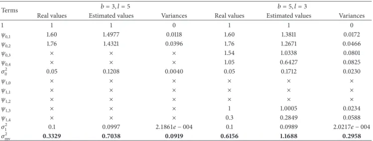
Table 1: The obtained model coefficients and minimum variance by linear estimation method.
Terms 𝑏 = 3, 𝑙 = 5 𝑏 = 5, 𝑙 = 3
Real values Estimated values Variances Real values Estimated values Variances
1 1 1 0 1 1 0 𝜓0,1 1.60 1.4977 0.0118 1.60 1.3811 0.0172 𝜓0,2 1.76 1.4321 0.0396 1.76 1.2671 0.0466 𝜓0,3 × × × 1.54 1.0338 0.0801 𝜓0,4 × × × 1.05 0.6427 0.0825 𝜎2 0 0.05 0.1208 0.0040 0.05 0.1712 0.0230 𝜓1,0 × × × × × × 𝜓1,1 × × × × × × 𝜓1,2 × × × × × × 𝜓1,3 × × × 1 1.0005 0.0234 𝜓1,4 × × × 0.3 0.2849 0.0588 𝜎2 1 0.1 0.0997 2.1861𝑒 − 004 0.1 0.0989 2.0217𝑒 − 004 𝜎2 mv 0.3329 0.7038 0.0919 0.6156 1.1688 0.2958
the variance decomposition. Firstly, two random vectors,
̇𝑥
(𝑘) = [ ̇𝑥(𝑘)
1 , ̇𝑥(𝑘)2 ]𝑁𝑡×1 and ̈𝑥
(𝑘) = [ ̈𝑥(𝑘)
1 , ̈𝑥(𝑘)2 ]𝑁𝑡×1, are
generated, which are two sets of𝑁mc simulation of
multi-dimensional inputs that have the requisite distribution.𝑁𝑡 denotes memory length of the model. Then, the mean and variance of𝑦𝑡+𝑏given the initial condition𝐼0can be calculated by ̂𝑦𝑡+𝑏| 𝐼0≅ 1 𝑁 𝑁mc ∑ 𝑘=1 𝑓2( ̇𝑥(𝑘)) | 𝐼 0; ̂ 𝑉𝑥| 𝐼0≅ 1 𝑁 𝑁mc ∑ 𝑘=1 (𝑓2( ̇𝑥(𝑘)) | 𝐼0)2− (̂𝑦𝑡+𝑏| 𝐼0)2. (51)
The partial variances can be estimated as
̂ 𝑉1| 𝐼0≅ 1 𝑁 𝑁mc ∑ 𝑘=1 𝑓2( ̇𝑥(𝑘)1 , ̇𝑥(𝑘)2 ) 𝑓2( ̇𝑥(𝑘)1 , ̈𝑥(𝑘)2 ) − (̂𝑦𝑡+𝑏| 𝐼0)2, ̂ 𝑉2| 𝐼0≅ 1 𝑁 𝑁mc ∑ 𝑘=1 𝑓2( ̇𝑥(𝑘)1 , ̇𝑥(𝑘)2 ) 𝑓2( ̈𝑥(𝑘)1 , ̇𝑥(𝑘)2 ) − (̂𝑦𝑡+𝑏| 𝐼0)2, ̂ 𝑉12| 𝐼0≅ ̂𝑉𝑥| 𝐼0− ̂𝑉1| 𝐼0− ̂𝑉2| 𝐼0. (52) To calculate the𝑉̂1 | 𝐼0with the different initial conditions, the average of these values can be used as the estimates of 𝐸𝐼0[𝑉1 | 𝐼0], and the performance index of nonlinear feedforward and feedback control system can be obtained.
5. Simulation Study
This section presents a simulation experiment to show the effectiveness of the proposed strategy. The model of nonlinear feedforward and feedback control system that we have chosen is expressed as
𝑦𝑡= 𝑓 (𝑢∗𝑡−𝑏) + 𝐷0,𝑡+ 𝑞−3(1 − 0.6𝑞−1) 𝐷1,𝑡, (53)
where𝑓(𝑢∗𝑡−𝑏)is process model represented by a nonlinear polynomial:
𝑓 (𝑢∗
𝑡−𝑏) = 0.2𝑢𝑡−3+ 0.3𝑢𝑡−4+ 𝑢𝑡−5+ 0.8𝑢2𝑡−3
+ 0.8𝑢𝑡−3𝑢𝑡−4− 0.7𝑢2𝑡−4− 0.5𝑢2𝑡−5− 0.5𝑢𝑡−3𝑢𝑡−5. (54) The measured and unmeasured disturbances are, respectively, given by
𝐷0,𝑡=1 − 1.6𝑞−11+ 0.8𝑞−2𝛼0.𝑡, 𝐷1,𝑡= 1 − 0.9𝑞1 −1𝛼1,𝑡,
(55) where {𝛼0,𝑡} and {𝛼1,𝑡} are sequences of independent and identically distributed normal variables with mean zero, and the variances are, respectively, 0.05 and 0.1.
Assume that the process is presently being controlled about a fixed set point by a simple proportional feedforward controller in addition to an integral feedback controller. The manipulated variable is given by
𝑢𝑡= −0.1𝐷1,𝑡−0.3 − 0.2𝑞−1
1 − 𝑞−1 𝑦𝑡. (56)
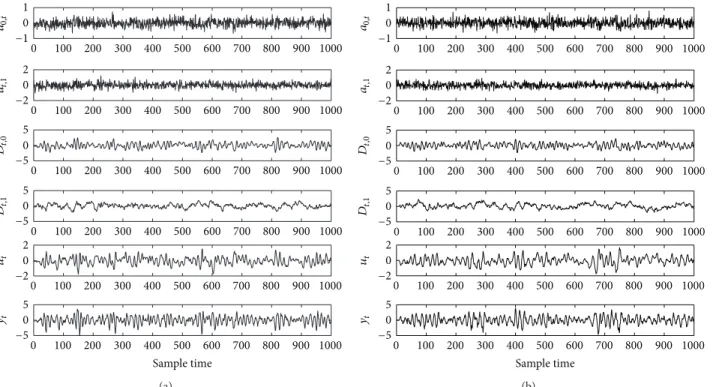
Two closed-loop signal curves of different time-delay condi-tions𝑏 = 3, 𝑙 = 5and𝑏 = 5, 𝑙 = 3are shown inFigure 2. Then, the traditional linear regression method is applied to estimate the MVPLB for nonlinear forward feedback control system. The estimated values of model parameters and MVPLB are shown inTable 1, where the model orders are𝐽0 = 7,𝐽1 = 7, and𝐽𝐷 = 1by applying AIC criterion and the values are calculated by 100 times’ statistics. It can be seen that the estimated value of model parameters and MVPLB by traditional linear regression method has larger deviation, which is always larger than the real value. This implies the excessive estimation.
It is necessary to identify the model of closed-loop system to estimate the minimum variance performance index of the
0 100 200 300 400 500 600 700 800 900 1000 0 100 200 300 400 500 600 700 800 900 1000 1 0 −1 2 0 −2 5 0 −5 yt ut Dt, 1 Dt, 0 at,1 a0,t Sample time 0 100 200 300 400 500 600 700 800 900 1000 0 100 200 300 400 500 600 700 800 900 1000 0 100 200 300 400 500 600 700 800 900 1000 0 100 200 300 400 500 600 700 800 900 1000 2 0 −2 5 0 −5 5 0 −5 (a) 0 100 200 300 400 500 600 700 800 900 1000 0 100 200 300 400 500 600 700 800 900 1000 1 0 −1 2 0 −2 5 0 −5 yt ut Dt, 1 Dt, 0 at,1 a0,t Sample time 0 100 200 300 400 500 600 700 800 900 1000 0 100 200 300 400 500 600 700 800 900 1000 0 100 200 300 400 500 600 700 800 900 1000 0 100 200 300 400 500 600 700 800 900 1000 2 0 −2 5 0 −5 5 0 −5 (b)
Figure 2: 1000 samples for the closed-loop nonlinear feedforward and feedback system subjected to measured and unmeasured disturbances. (a)𝑏 = 3,𝑙 = 5; (b)𝑏 = 5,𝑙 = 3. 300 350 400 450 500 550 600 650 700 750 5 4 3 2 1 0 −1 −2 −3 −4 −5 yt Sample time Output signals of real model Output signals of identified model
(a) 300 350 400 450 500 550 600 650 700 750 4 2 0 −2 −4 yt Sample time Output signals of real model Output signals of identified model
800 6
−6
(b)
Figure 3: Output signals of identified model comparing with actual model. (a)𝑏 = 3,𝑙 = 5; (b)𝑏 = 5,𝑙 = 3.
nonlinear system. First, we collect the disturbance signals which can be measured and then apply the linear regression method to fit the curve to obtain the parameter of the white noise. Furthermore, we use iterative orthogonal least square method to identify the closed-loop model. The comparison for the output signal of identified model and actual model under two different time delays is shown in Figure 3. We can see the identified model can well approximate to the real nonlinear model.
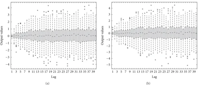
It is noted that the output variance of nonlinear system is also related to the initial value. Thus, to see whether the resulting controller performance based on variance decom-position method includes the influence of the initial value or not, the output variation of closed-loop system during the period𝑡 = 1, 2, . . . , 40is shown inFigure 4. It can be seen that when𝑡 > 20, the distribution of the system output tends to be stable; thus we get the conclusion that the output has nothing to do with the initial value.
1 3 5 7 9 11 13 15 17 19 21 23 25 27 29 31 33 35 37 39 4 3 2 1 0 −1 −2 −3 −4 Ou tp u t val ues Lag (a) 1 3 5 7 9 11 13 15 17 19 21 23 25 27 29 31 33 35 37 39 4 3 2 1 0 −1 −2 −3 −4 O u tput v alu es Lag −5 (b)
Figure 4: Box plots for closed-loop system output on memory length𝑡 = 1, . . . , 40. (a)𝑏 = 3,𝑙 = 5; (b)𝑏 = 5,𝑙 = 3.
1 2 3 1.2 1 0.8 0.6 0.4 0.2 Es tima tes o f p er fo rma nce indices Method (1) Theoretical performance index (2) Linear autoregressive method (3) Proposed method in this paper
(a) 1 2 3 1.2 0.8 0.6 0.4 0.2 Es tima tes o f p er fo rma nce indices Method 4 5 6 7 1.6 1.4 0
(1) Theoretical performance index (2) Contribution of unmeasured disturbance
with LAR method
(3) Contribution of measured disturbance with LAR method
(4) Performance index with LAR method (5) Contribution of unmeasured disturbance
with proposed method
(6) Contribution of measured disturbance with proposed method
(7) Performance index with proposed method
1
(b)
Figure 5: Box plots of the estimates of the minimum variance lower bound for the nonlinear feedforward and feedback control system. (a) 𝑏 = 3,𝑙 = 5; (b)𝑏 = 5,𝑙 = 3.
Selecting an appropriate memory length of 40 and apply-ing 100 times’ Monte Carlo experiments, the box plots of MVPLB estimates with time delay𝑏 = 3, 𝑙 = 5, and𝑏 = 5, 𝑙 = 3by applying variance decomposition method proposed by this paper and traditional linear estimation method can be seen in Figure 5. In Figure 5(a), the first column gives theoretical performance index for nonlinear system with time
delay𝑏 = 3, 𝑙 = 5, and the second column and third one, respectively, show the estimates of performance index by tra-ditional linear method and that by the method in this paper. InFigure 5(b), the first column gives theoretical performance index for nonlinear system with time delay𝑏 = 5, 𝑙 = 3, and the fourth column and seventh column, respectively, show the estimates of performance index by traditional linear
method and that by the method in this paper. The second and third column, respectively, show the contributions of perfor-mance index of the unmeasured and measured disturbance signal applying traditional linear method. The fifth and sixth column show the contributions of performance index of the unmeasured and measured disturbance signal applying the method proposed by this paper, respectively. From the plot, we can see that the estimates of performance index using our new method are more close to the theoretical value than that using traditional linear method and get the conclusion that it is effective to estimate the MVPLB of nonlinear forward and feedback system by applying the CPA method based on variance decomposition method.
Remarks.(i) The MVPLB of this nonlinear feedback and
for-ward control system can be decomposed into the best possible bounds for each of the controllers. According to the variance contributions of the unmeasured and measured disturbance, we can confirm the degree of controller performance by the feedback controller and the feedforward controller.
(ii) When the feedforward delay exceeds the feedback delay, there is no error in predicting of the future disturbance by using given information at current time. In such case, the overall MVPLB is only the contribution of unmeasured disturbance. This is the reason why only three columns are included inFigure 5.
(iii) This new nonlinear CPA method requires only observable signals and crude estimates of the process delay and another delay that it takes for a change in measured feedforward variable to begin to affect the output.
(iv) The proposed method needs to estimate the loop nonlinear model, and the identification of the closed-loop model will directly affect the estimates of the MVPLB.
6. Conclusions
The problem of control performance assessment for non-linear feedforward and feedback system is investigated in this paper. We provide a method based on the variance decomposition to estimate the MVPLB for two classes of nonlinear feedforward and feedback control system. When the time delay of the process and measured disturbance are known, the performance index based on minimum variance benchmark can be estimated by the data from the closed-loop system; the simulation shows the effectiveness of the proposed approach. More specifically, the assumption of one measured disturbance is also suitable for the multimeasured disturbance cases; thus the method in this paper can be extended from SISO to MISO.
Conflict of Interests
The authors declare that there is no conflict of interests regarding the publication of this paper.
Acknowledgments
This work was supported by the Priority Academic Program Development of Jiangsu Higher Education Institutions and
the 111 Project (B12018) and the Basic Research Program of Jiangsu Province of China (Natural Science Foundation) (BK2012111).
References
[1] T. J. Harris, “Assessment of control loop performance,” The Canadian Journal of Chemical Engineering, vol. 67, no. 5, pp. 856–861, 1989.
[2] L. Desborough and T. Harris, “Performance assessment mea-sures for univariate feedback control,”The Canadian Journal of Chemical Engineering, vol. 70, no. 6, pp. 1186–1197, 1992. [3] N. Stanfelj, T. E. Marlin, and J. F. MacGregor, “Monitoring and
diagnosing process control performance: the single-loop case,”
Industrial and Engineering Chemistry Research, vol. 32, no. 2, pp. 301–314, 1993.
[4] L. Desborough and T. Harris, “Performance assessment mea-sures for univariate feedforward/feedback control,”The Cana-dian Journal of Chemical Engineering, vol. 71, no. 4, pp. 605–616, 1993.
[5] T. J. Harris, F. Boudreau, and J. F. MacGregor, “Performance assessment of multivariable feedback controllers,”Automatica, vol. 32, no. 11, pp. 1505–1518, 1996.
[6] B. Huang, S. L. Shah, and E. K. Kwok, “Good, bad or optimal? Performance assessment of multivariable processes,” Automat-ica, vol. 33, no. 6, pp. 1175–1183, 1997.
[7] B. Huang, S. L. Shah, and R. Miller, “Feedforward plus feedback controller performance assessment of MIMO systems,”IEEE Transactions on Control Systems Technology, vol. 8, no. 3, pp. 580–587, 2000.
[8] S. J. Qin, “Control performance monitoring—a review and assessment,”Computers and Chemical Engineering, vol. 23, no. 2, pp. 173–186, 1998.
[9] B. Huang and S. L. Shah,Performance Assessment of Control Loops: Theory and Applications, Springer, London, UK, 1999. [10] M. Jelali, “An overview of control performance assessment
technology and industrial applications,” Control Engineering Practice, vol. 14, no. 5, pp. 441–466, 2006.
[11] B. Srinivasan, T. Spinner, and R. Rengaswamy, “Control loop performance assessment using detrended fluctuation analysis (DFA),”Automatica, vol. 48, no. 7, pp. 1359–1363, 2012. [12] R. Gonzalez and B. Huang, “Control loop diagnosis with
ambiguous historical operating modes: part 1. A proportional parametrization approach Original Research Article,”Journal of Process Control, vol. 23, no. 4, pp. 585–597, 2013.
[13] R. Gonzalez and B. Huang, “Control loop diagnosis with ambiguous historical operating modes: part 2, information synthesis based on proportional parametrization,”Journal of Process Control, vol. 23, no. 10, pp. 1441–1454, 2013.
[14] S. Liu, J. F. Fiu, Y. P. Feng et al., “Performance assessment of decentralized control systems: an iterative approach,”Control Engineering Practice, vol. 22, pp. 252–263, 2014.
[15] T. J. Harris and W. Yu, “Controller assessment for a class of non-linear systems,”Journal of Process Control, vol. 17, no. 7, pp. 607– 619, 2007.
[16] W. Yu, D. I. Wilson, and B. R. Young, “Nonlinear control performance assessment in the presence of valve stiction,”
Journal of Process Control, vol. 20, no. 6, pp. 754–761, 2010. [17] W. Yu, D. I. Wilson, and B. R. Young, “Control performance
assessment for nonlinear systems,”Journal of Process Control, vol. 20, no. 10, pp. 1235–1242, 2010.
[18] Z. Zhang, On Performance assessment for nonlinear control systems based on mimimum variance benchmark [Ph.D. thesis], Shanghai Jiao Tong University, Shanghai, China, 2013. [19] W. Yu, D. I. Wilson, and B. R. Young, “Control performance
assessment for a class of nonlinear multivariable systems,”
Computer Aided Chemical Engineering, vol. 30, pp. 962–966, 2012.
[20] W. Yu, D. Wilson, B. Young, and T. Harris, “Variance decom-position of nonlinear systems,” in Proceedings of the IEEE International Conference on Control and Automation (ICCA ’09), pp. 738–744, Christchurch, New Zealand, December 2009. [21] G. E. B. Archer, A. Saltelli, and I. M. Sobol, “Sensitivity measures, anova-like techniques and the use of bootstrap,”
Journal of Statistical Computation and Simulation, vol. 58, no. 2, pp. 99–120, 1997.
[22] S. Chen, S. A. Billings, and W. Luo, “Orthogonal least squares methods and their application to nonlinear system identifica-tion,”International Journal of Control, vol. 50, no. 5, pp. 1873– 1896, 1989.
Submit your manuscripts at
http://www.hindawi.com
Hindawi Publishing Corporation
http://www.hindawi.com Volume 2014
Mathematics
Journal ofHindawi Publishing Corporation
http://www.hindawi.com Volume 2014 Mathematical Problems in Engineering
Hindawi Publishing Corporation http://www.hindawi.com
Differential Equations
International Journal of Volume 2014
Hindawi Publishing Corporation
http://www.hindawi.com Volume 2014 Hindawi Publishing Corporationhttp://www.hindawi.com Volume 2014
Hindawi Publishing Corporation
http://www.hindawi.com Volume 2014
Mathematical PhysicsAdvances in
Complex Analysis
Journal of Hindawi Publishing Corporationhttp://www.hindawi.com Volume 2014
Optimization
Journal ofHindawi Publishing Corporation
http://www.hindawi.com Volume 2014
Combinatorics
Hindawi Publishing Corporation
http://www.hindawi.com Volume 2014
International Journal of Hindawi Publishing Corporation
http://www.hindawi.com Volume 2014
Journal of
Hindawi Publishing Corporation
http://www.hindawi.com Volume 2014
Function Spaces
Abstract and Applied Analysis Hindawi Publishing Corporation
http://www.hindawi.com Volume 2014 International Journal of Mathematics and Mathematical Sciences
Hindawi Publishing Corporation http://www.hindawi.com Volume 2014
The Scientific
World Journal
Hindawi Publishing Corporation
http://www.hindawi.com Volume 2014
Hindawi Publishing Corporation
http://www.hindawi.com Volume 2014
Discrete Dynamics in Nature and Society
Hindawi Publishing Corporation
http://www.hindawi.com Volume 2014
Hindawi Publishing Corporation
http://www.hindawi.com Volume 2014
Discrete Mathematics
Journal ofHindawi Publishing Corporation
http://www.hindawi.com Volume 2014 Hindawi Publishing Corporationhttp://www.hindawi.com Volume 2014