A Goal Programming Model for Single Vehicle Routing Problem with Multiple Routes

(1)

Vol. 2, No. 2, pp 154-163 Summer 2008

A Goal Programming Model for Single Vehicle Routing Problem with

Multiple Routes

Fariborz Jolai*, Mehdi Aghdaghi

Industrial Engineering Department, Faculty of Engineering, University of Tehran, P.O. Box 11365-4563 [email protected]

ABSTRACT

The single vehicle routing problem with multiple routes is a variant of the vehicle routing problem where the vehicle can be dispatched to several routes during its workday to serve a number of customers. In this paper we propose a goal programming model for multi-objective single vehicle routing problem with time windows and multiple routes. To solve the model, we present a heuristic method which exploits an elementary Shortest Path Algorithm with Resource Constraints. Computational results of the proposed algorithm are discussed.

Keywords: Single vehicle, Routing problem, Multiple routes, Time windows, Goal programming,

1. INTRODUCTION

Vehicle Routing Problem (VRP) is a well known combinatorial optimization problem arising in transportation management and logistics. VRP involves the determination of a set of routes for a fleet of vehicles, starting and ending at a depot and serving a set of customers with known demands. Each customer must be visited by one of these routes and all the customers must be assigned to vehicles such that the restrictions on the capacity of vehicles and the duration of a route are met. The objective of the problem is to minimize the total cost of the set of routes.

Some vehicle routing problems have pre-set time constraints on the periods of the day in which customers should be served. They are known as Vehicle Routing Problem with Time Window (VRPTW) (Calvete et al., 2007; Hashimoto et al., 2006; Hong and Park, 1999; Ombuki et al., 2006; and Solomon, 1987).

A variant of VRP which has received little attention in the literature in spite of its importance in practice is a problem where the same vehicle can perform several routes during a workday. For example, in the home delivery of perishable goods, like food, routes are of short duration and must be combined to form a complete workday. Azi et al. (2006) proposed an exact algorithm for a single-vehicle routing problem with time windows and multiple routes.

The real-life distribution and transportation problems have other objectives than minimizing the total travel cost (time or distance). Hence great attention has been paid to multiple objectives VRP

*

(2)

in the past years (Calvete et al., 2007; Hong and Park, 1999; Lacomme et al., 2006; Ombuki et al., 2006; and Tan et al., 2006). The goal programming (GP) approach is an important technique to model multi-objective problems and helps decision-makers to solve multi-objective decision making problems in finding a set of satisfying solutions. The purpose of GP is to minimize the deviations between the achievement of goals and their aspiration levels. Hong and Park (1999) and Calvete et al. (2007) used goal programming approach to model the VRPTW.

In this paper we present a goal programming model for single vehicle routing problem with time windows and multiple routes. The remainder of the paper is organized as follows. In Section 2, the mathematical formulation of single vehicle routing problem with time windows and multiple routes is described as a goal programming model. In Section 3, a heuristic algorithm to solve the model is proposed. In Section 4, we carry out some experiments using a set of data obtained from Solomon’s instances. Finally in Section 5, we describe some overall conclusions.

2. THE MODEL

We formulate the problem on a directed network as follow.

Let

N

=

{

1 ,

2 ,...,

n

}

be a set of nodes (each representing a customer location). We define

)

,

(

N

A

G

′

as a directed graph associated with the problem, where

N

′

=

{

0 }

_U

N

_U

{

n

+

1 }

is the set of nodes and

A

=

{(

i

,

j

)

:

i

,

j

∈

N

′

}

is the set of directed arcs (all possible connections between the nodes). Index 0 refers to the central depot, while index n+1 refers to a virtual node which is a copy of depot.

Each node

i

is associated with a known demand

q

i and also with a known service time

s

i. For nodes

0 and n+1 we have

q

0

=

q

n+1

=

0

and

s

0

=

s

n+1

=

0

. Let[ai,bi]be a time interval during which

service of customer

i

has to take place (time window).

Each arc

(

i

,

j

)

∈

A

is associated with a travel timetij and travel costcij, represent time and cost of

going from node

i

to node

j

through arc(i,j). For virtual arcs between node 0 and noden+1, we have

0

1 , 0 1 ,

0n+

=

t

n+

=

c

.

There is a single vehicle of capacity Udelivering goods from the depot to the customers. Let’s define the vehicle workday by a set of routes

R

=

{

1 ,

2 ,...,

r

}

. Each route originates at node 0 and terminates at noden+1. The number of routes in the set

R

is not apparent before solving the problem. Hence we set the size of set

R

with maximum number of routes which can be defined to serve all customers. It should be noted that some of these routes might contain no customer, i.e. they are dummy routes. For each routek∈R we define vehicle loading time

L

kas a function of total service time of all customers in routek. In some applications, like the home delivery of perishable goods, routes cannot be too long. So we can assume every customer in a route must be served before a given deadline,

T

_max, associated with that route.

(3)

Goal (1) Minimize the total cost to serve the customers.

Goal (2) Maximize the number of served customers.

Goal (3) Minimize the total waiting time (at customers’ locations or at depot).

Goal (4) Avoid underutilization of vehicles capacity.

Also to formulate the model we define the following variables:

R k A j i

xijk, (, )∈ , ∈ is equal to 1 if route k contains arc (i,j)and 0 otherwise.

R

k

N

i

y

_ik

,

∈

′

,

∈

is equal to 1 if node

i

is in routekand 0 otherwise.

N

i

w

i

,

∈

, specifies start time of service at node

i

.

R

k

w

k n k

∈

+

,

₁

0 stand for the start time and end time of routek, respectively.

) 4 ( ) 3 ( ) 2 ( ) 1 (

,

n

i

p

n

k

p

represent deviational variables of the goals.

Given the above goals and variables we formulate the goal programming model of the problem as follow:

∑

∈ ∈

+

R k k N i

i

p

n

p

(1) (2) (2) (3) (3) (4) (4) )

1 (

min

ω

₍₀₎

st: 0 ) 1 ( ) , (

C

p

x

c

R k k ij A j i

ij

∑

−

=

∑

∈ ′

∈ (1)

∑

∈

∀

=

) (

,

i j k i k

ij

y

i

N

k

R

x

β (2)

∑

∈

∀

=

+

R k i k

i

n

i

N

y

(3)

1

₍₃₎

R

k

N

i

x

i

i i i

k ji k

ij

−

=

∀

∈

′

∀

∈

∑

∈ ∈

,

0

) ( ()

β α (4)

R

k

x

j k

j

≤

∀

∈

∑

∈

1

) 0 ( 0

β (5)

R

k

x

n i k n

i

=

∀

∈

∑

+ ∈ +

1

) 1 ( 1 ,

β (6)

N

i

b

w

a

_i

≤

_i

≤

_i

∀

∈

(7)

R k y s x t TR n i n j n i k i i k ij ij

k =

∑∑

+

∑

∀ ∈ = + = = 0 1 1 1 (8) 0 ) ( )

( ₁− ₀ − + ₀ 1 − ₊₁ − (3) = ∈

+

∈ +

∑

w w TR w w_nk p

R k k k k R k k

n (9)

R

k

U

n

y

q

_ik _k N

i

+

=

∀

∈

∑

∈ ) 4 ( (10)

A

j

i

x

M

t

s

w

R k k ij ij i i

j

−

≤

−

∑

∀

∈

)

,

(

)

1 (

₍₁₁₎

A

j

i

x

M

t

s

w

R k k ij ij i i

j

−

≥

−

∑

∀

∈

)

,

(

)

1 (

₍₁₂₎

(4)

} 1 { ,

) 1 ( ₀ 0

0 + + − ∀ ∈ ∈ +

≤w t M x k R j N n

w j kj

k

j U (13)

} 1 { ,

) 1 ( 0 0

0 + − − ∀ ∈ ∈ +

≥w t M x k R j N n

w j kj

k

j U (14)

1 1

0

L

w

≥

(15)

R

k

L

w

₀k+1

≥

_nk₊₁

+

k+1

∀

∈

(16)

R k y

s L

N i

k i i

k ₌

∑

_∀ _∈

∈ (17)

R

k

T

w

_nk₊₁

≤

₀k

+

_max

∀

∈

(18)

R k A j i

xijk ∈{0,1} ∀(, )∈ , ∈ (19)

R

k

N

i

y

ik

∈

{

0 ,

1 }

∀

∈

,

∈

(20)

Constraint (1) which includes a positive deviational variable

p

(1)corresponds to goal (I). This constraint allows us to assign a penalty to a deviation from a targeted total delivery cost

C

0.

Constraint (2) guarantees that

y

_ik is equal to 1 when node

i

is in routek. Constraint (3) refers to Goal (2) and states that every customer can only be visited once. Sum of the negative deviational variable

∑

ni(2) which is weighted by

) 2 (

ω

in the objective function, computes the number of

customers who have not been served. Both constraints (3) and (4) make sure that exactly one arc enters and leaves each served customer. Analogously, constraints (5) and (6) ensure that all routes leave the depot (node 0) and return to it (noden+1). Constraint (7) refers to time windows of customers. Constraints (8) and (9) allow us to formulate Goal (3). Constraint (10) corresponds to the vehicle capacity constraint and represents Goal (4) by using negative deviational variables

n

k(4).

Constraints (11)-(16) ensure feasibility of the time schedule. Constraint (17) computes vehicle loading time in routek and finally, constraint (18) ensures that every customer in a routek must be served before

T

_max.

The proposed model faces with difficulties on account of large number of variables and constraints. So it is necessary to develop an algorithm capable of solving large sized problem.

3. SOLUTION METHOD

To solve the problem we develop an algorithm with goal programming approach which exploits the contexts of a shortest path algorithm with resource constrain, as proposed by Azi (2006).

In the shortest path algorithm with resource constraints a path is characterized by its length and the consumption of each resource. In this algorithm, the consumed resource is a criterion to compare the performance of the routes, e.g., in VRPTW the time windows can be defined as a resource. When different paths visit the same nodes, a path might well be better than some other paths, over all criteria. The dominance relation in the shortest path algorithm with resource constraint is defined as follows.

Path

p

dominates

p

′

if (1) it is not longer, (2) it does not consume more resources for every resource considered and (3) every unreachable node for

p

is also unreachable for path

p

′

. By

(5)

eliminating paths through this dominance relation, only labels corresponding to non-dominated elementary paths are kept and a solution to the problem is obtained at the end.

Our problem-solving approach, based on this algorithm, is divided into two phases. In the first phase, feasible routes are constructed. Then, in the second phase some of these routes are combined to form a workday for the vehicle. Therefore, the routing issues are decoupled from the scheduling issues of a workday. That is, when a route is known, the sum of the service times and the setup times are known.

Phase 1

In Phase1 we want to generate a set of feasible routes which will be used in the second phase. In our algorithm, a path is characterized by the set of its nodes and value of each goal. More precisely, a path

p

is labeled with R_p =(d_p,y1_p,...,yn_p,o1_p,...og_p) where

d

p is the number of nodes in

path

p

, yip =1 if node

i

is in path

p

, 0 otherwise,

G

=

{

1 ,

2 ,...,

g

}

is the set of goals and k p o is the value of goalk. If all goals of the problem must be minimized, we can define dominance relation as follow.

The dominance relation (Azi, 2006): If

p

and

p

′

are two different paths with labels

R

_p and

R

_p_′ , respectively, then path

p

dominates

p

′

if and only if

d

_p_′

≤

d

_p, yi_p_′ ≤ yi_p i=1,...,n,

g k

o

ok_p_′ ≥ k_p =1,... .

A path

p

thus dominates another path

p

′

if

p

contains all nodes of

p

′

(although in a different order), and

p

is better than

p

′

, for every goal considered.

The algorithm generates all feasible routes and uses the proposed dominance relation to make a set of routes for Phase 2.

Phase 2

The contexts of shortest path algorithm proposed in Phase 1, will be used again in Phase 2 to create a workday for the vehicle. Here we make a transformed graph where the nodes correspond to the routes generated in Phase 1, plus two artificial nodes that correspond to the start and end of the vehicle workday. In the graph, there is an arc between nodes

r

and

r

′

if (1) the two subsets of customers in routes

r

and

r

′

are disjoint and (2) it is feasible to serve route

r

′

after route

r

. The feasibility is checked through time windows of nodes

r

and

r

′

. The departure time interval associated with each route is used for this purpose. That is, if node

r

′

is placed after node

r

, the vehicle must be back at the depot from route

r

and be ready to depart before the latest departure time of route

r

′

. If the vehicle is ready before the earliest departure time, then it must wait. Hence, to use the shortest path algorithm in Phase 2 we need to determine the feasible time intervals of departure from the depot for every route

r

. These feasible time intervals are used as time windows of nodes in the graph. Let us denote the earliest and the latest departure times of route

r

as a time interval

[

θ

₀r

,

τ

₀r

]

, analogously, the earliest and latest return times

[

θ

_nr₊₁

,

τ

_nr₊₁

]

.

(6)

Let n_r denote the number of customers in the route

r

. We define the sequence

(

₀

,

₁

,...,

,

₊₁

)

r r n n

i

for route

r

to represent the sequence of customers (

i

0

=

0

and

i

n_r+1

=

n

+

1

). The latest feasible

time to begin service at customer

i

j in route

r

is denoted by r i_j

τ

. For the depot,

τ

ir₀ =

τ

0r and r

n r

i_n_r+₁

=

τ

+1

τ

are the latest feasible departure and arrival times, respectively. To determine time interval

[

1

,

1

]

r n r n+

τ

+

θ

of each route

r

, we apply a backward sweep and compute

the value of _ir

j

τ

for every

i

_jof customer sequence in route

r

. Then we apply a forward sweep and reset the value of

τ

ir_j.

The backward sweep of route

r

is applied from

i

n_r+1 to

i

0

=

0

. First, in node

i

n_r+1 the algorithm

sets

1 1 + +

=

nr r

n i

r i

b

τ

then sweeps to previous nodes and computes

τ

ir_jfor node

i

jas follows: 0

,

}

,...,

min{

1

t

j j

s

j

b

j

i

r

i

j

j i i i i n

r i r

i

=

τ

+

−

+

−

=

τ

Where

j i

b is the upper bound of time window corresponding to customer

i

_j.

It should be noted that for virtual noden+1, we can set ₊

=

+∞

1 r n i

b

. At the end of the backward

sweep, in node

i

₀ algorithm obtains _ir

0

τ

. Once _ir

0

τ

has been obtained, a forward sweep is applied to get the latest feasible schedule. The _ir

j

τ

values will be reset as follow:

1 1

1

,

}

,...,

max{

₋

+

₋

+

₋_,

=

₁ ₊

=

r j j j j j

j i i i i n

r i r

i

τ

s

t

a

j

i

τ

Where

j i

a is the lower bound of time window corresponding to customer

i

_j.

Now for each path

r

, we determine the latest feasible departure time ir r

0 0

τ

= and the latest feasible

return time _nr _ir

r n r+1

=

τ

+1

τ

. To compute the earliest departure times,

θ

₀r, and the earliest return

times,

θ

_nr₊₁, we should consider two cases. Case 1 happens when there is no waiting time in the latest feasible schedule of route

r

. Since the departure time of route

r

can be shifted backward by

r

δ

time units, and since we have

min{

,...,

}

1 1 0

0

−

+

−

+

=

r n r n i r i i r i r

a

τ

δ

, then we can set

r r r

τ

δ

θ

0

=

0

−

and

r r n r

n

τ

δ

θ

₊1

=

₊1

−

. In case 2 there is some waiting time in the latest feasible

schedule and it is not possible to depart earlier from the depot without increasing the route duration. Hence

θ

0r

=

τ

0r and

r n r

n+1

=

τ

+1

θ

. Now we use our approach which was described in phase 1, to find

an elementary path with best value of goals. The departure time windows associated with each route are used for this purpose. That is, the vehicle must be back at the depot and ready to depart before the latest departure time of its next route. If the vehicle is ready before the earliest departure time,

(7)

then it must wait. When arc (

r

′

,

r

′

) is added to the current path, route

r

′

is included into the vehicle workday.

4. COMPUTATIONAL RESULTS

In this section we present the experimental results performed by applying the proposed algorithm on some instances of problem. Since there is only one vehicle, it can not serve a large number of customers during one day. Hence the instances are constructed by taking only the first 25 and 50 customers of Solomon’s instances C2, R2 and RC2 (1987). Also we create some small size

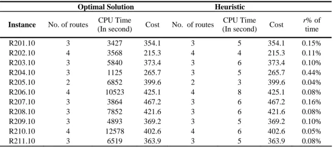
Table 1: Comparison with optimal solution

Optimal Solution Heuristic

Instance No. of routes CPU Time

(In second) Cost No. of routes

CPU Time

(In second) Cost

r% of time

R201.10 3 3427 354.1 3 5 354.1 0.15% R202.10 4 3568 215.3 4 4 215.3 0.11% R203.10 3 5840 373.4 3 6 373.4 0.10% R204.10 3 1125 265.7 3 5 265.7 0.44% R205.10 2 6852 399.6 2 3 399.6 0.04% R206.10 4 10523 425.1 4 8 425.1 0.08% R207.10 3 3864 467.2 3 6 467.2 0.16% R208.10 3 7852 421.6 3 6 421.6 0.08% R209.10 3 4893 369.2 3 5 369.2 0.10% R210.10 4 12578 402.6 4 6 402.6 0.05% R211.10 3 6519 363.9 3 5 363.9 0.08%

Table 2: Experimental results with T

max

=220

Phase 1 Phase 2 Goal (1) Goal (2)

Instance No. of routes

CPU Time (In second)

No. of routes

CPU Time

(In second) Cost

No. of served customer

C201.25 97 3 10 1 279.4 23

C201.50 227 11 11 10 325.5 27

C202.25 287 9 10 6 259.6 22

C202.50 1021 26 12 366 324.9 28

C203.25 367 15 12 19 295.3 25

C203.50 1672 658 11 1820 305.5 29

C204.25 525 13 10 33 380.5 25

C204.50 2121 1326 11 4330 365.1 29

C205.25 107 5 9 1 305.9 24

C205.50 512 35 10 45 295.4 26

C206.25 166 1 11 1 367.2 24

C206.50 603 45 11 99 339.2 29

C207.25 103 10 10 11 258 23

C207.50 1011 1050 12 549 303.1 29

C208.25 117 9 10 5 328.6 24

(8)

problems by taking the first 10 customers from instances R2 to evaluate performance of the presented heuristic algorithm in comparison to the optimal solutions. The heuristic algorithm discussed in this paper was coded and run on a PC Pentium iii, 800MHz, 512 MB Ram.

The results reported in Table1 show that the heuristic leads to optimal solutions in reasonable time (

T

_max

=

75

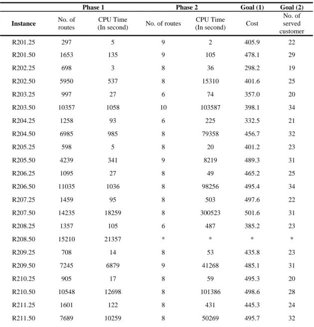
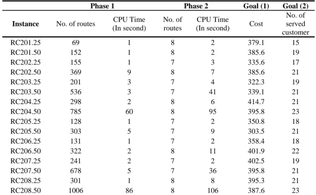
). It is apparent that CPU time of Phase 2 depends on the number of routes in Phase 1. Tables 2-4 show the results of computational experiments with different Tmax values and problem

instances. Table 2 shows the results of C2 and

T

_max

=

220

, Table 3 shows the results of R2 and

90

max

=

T

. The results of RC2 with

T

_max

=

75

are given in Table 4. In these tables the numbers of routes in phase 1 and in phase 2 are given. Finally Table 5 summarizes all results.

Table 3: Experimental results with T

max

=90

Instance No. of routes

CPU Time

(In second) No. of routes

CPU Time

(In second) Cost

R201.25 297 5 9 2 405.9 22

R201.50 1653 135 9 105 478.1 29

R202.25 698 3 8 36 298.2 19

R202.50 5950 537 8 15310 401.6 25

R203.25 997 27 6 74 357.0 20

R203.50 10357 1058 10 103587 398.1 34

R204.25 1258 93 6 225 332.5 21

R204.50 6985 985 8 79358 456.7 32

R205.25 598 5 8 20 401.2 23

R205.50 4239 341 9 8219 489.3 31

R206.25 1095 27 8 49 465.2 25

R206.50 11035 1036 8 98256 495.4 34

R207.25 1459 95 8 503 497.6 22

R207.50 14235 18259 8 300523 501.6 31

R208.25 1357 105 6 487 385.2 23

R208.50 15210 21357 * * * *

R209.25 708 14 8 53 435.8 23

R209.50 7245 6879 9 41268 485.1 31

R210.25 905 17 8 59 495.3 20

R210.50 10548 12698 8 101386 498.6 28

R211.25 1601 122 8 431 445.3 24

(9)

Table 4: Experimental results with T

max

=75

Instance No. of routes CPU Time

(In second)

No. of routes

CPU Time

(In second) Cost

RC201.25 69 1 8 2 379.1 15

RC201.50 152 1 8 2 385.6 19

RC202.25 155 1 7 3 335.6 17

RC202.50 369 9 8 7 385.6 21

RC203.25 201 3 7 4 322.3 19

RC203.50 536 3 7 41 339.1 21

RC204.25 298 2 8 6 414.7 21

RC204.50 785 60 8 95 395.8 23

RC205.25 128 1 7 2 350.8 18

RC205.50 303 5 7 9 303.5 21

RC206.25 131 1 7 2 358.4 18

RC206.50 322 2 8 11 401.9 22

RC207.25 241 2 7 2 402.5 19

RC207.50 678 5 7 36 395.8 21

RC208.25 301 1 8 8 395.3 21

RC208.50 1006 86 8 106 387.6 23

Table 5 : The summary of results with different problem sets

Phase 1 Phase 2

Ave of routes

Ave of CPU Time (In second)

Ave of routes

Ave of CPU Time (In second)

Ave of served customer

C2.25 221.1 8.1 10.3 9.6 23.8

R2.25 997.5 46.6 7.5 176.3 22.0

RC.25 190.5 1.5 7.4 3.6 18.5

C2.50 981.1 434.5 11.1 939.8 28.3 R2.50 8649.6 6685.8 8.5 79828.1 30.7

RC2.50 518.9 21.4 7.6 38.4 21.4

Average number of routes in Phase 1 is 469.72 for instances with 25 customers and is 3383.21 for instances with 50 customers. These tables show the impact of using dominance relation and

T

max on

the number of feasible routes in Phase 1.

5. CONCLUSION

In this paper we proposed a linear goal programming model for a variant of vehicle routing problem with time windows (VRPTW) where a vehicle can perform several routes during its workday. This variant of VRPTW is called single vehicle routing problem with time windows and multiple routes. We also proposed a heuristic based on shortest path algorithm to solve the multi-objective problem. The proposed algorithm is capable of solving medium-size VRP’s which include around 50

(10)

customers. As a future development we suggest improving our algorithm to solve large instances of VRP.

REFERENCES

[1] Azi N., Gendreau M., Potvin J. (2006), An exact algorithm for a single-vehicle routing problem with time windows and multiple routes; European Journal of Operational Research; Article in press. [2] Calvete H.I., Gale C., Oliveros M.J. (2007), Valverde B.S., A goal programming approach to vehicle

routing problems with soft time windows; European Journal of Operational Research 177; 1720-1733. [3] Fisher M.L (1994), Optimal solution of vehicle routing problems using minimum k-trees; Operation

Research 42; 626-642.

[4] Hashimoto H., Ibaraki T., Imahori S., Yagiura M. (2006), The vehicle routing problem with flexible time windows and traveling times; Discrete Applied Mathematics 154; 1364-1383.

[5] Hong S.C., Park Y.B (1999), A heuristic for bi-objective vehicle routing with time window constraints; International Journal of Production Economics 62; 249-258.

[6] Irnich S., Funkeb B., Grünert T. (2006), Sequential search and its application to vehicle-routing problems; Computers & Operations Research 33; 2405–2429.

[7] Lacomme P., Prins C., Sevaux M. (2006), A genetic algorithm for a bi-objective capacitated arc routing problem; Computers and Operations Research 33; 3473-3493.

[8] Laporte G., Nobert Y. (1987), Exact algorithms for the vehicle routing problem; Annals of Discrete Mathematics 31; 147-184.

[9] Miller D.L. (1995), A matching based exact algorithm for capacitated vehicle routing problem; ORSA Journal on Computing 7; 1-9.

[10] Ombuki B., Ross B.J., Hanshar F. (2006), Multi-Objective Genetic Algorithms for Vehicle Routing Problem with Time Windows; Applied Intelligence 24; 17–30.

[11] Solomon M. (1987), Algorithms for the vehicle routing and scheduling problems with time window constraints; Operations Research 35; 254–65.

[12] Tan K.C., Chew Y.H., Lee L.H. (2006), A hybrid multi-objective evolutionary algorithm for solving truck and trailer vehicle routing problems; European Journal of Operational Research 172; 855-885. [13] Toth P., Vigo D. (Eds.) (2002), The Vehicle Routing Problem; SIAM Monographs on Discrete