Vol. 6, No. 1, pp 77-87
Testing Exponentiality Based on Record
Values
A. Habibi Rad, F. Yousefzadeh, M. Amini, N. R. Arghami
Department of statistics, School of Mathematical Sciences, Ferdowsi Univer-sity of Mashhad, Iran. ([email protected], yousefzadeh [email protected], [email protected], [email protected])
Abstract. We introduce a goodness of fit test for exponentiality based on record values. The critical points and powers for some alternatives are obtained by simulation.
1
Introduction
Suppose a random variable X has cumulative distribution function (cdf)F(x) and a continuous probability density function (pdf)f(x). The entropyH(f) of the random variableX is defined in [10] to be
H(f) =− Z ∞
−∞
f(x) logf(x)dx. (1)
The Kullback-Leibler (K-L) information of f(x) against f0(x) is defined in [7] to be
I(f;f0) =
Z ∞
−∞
f(x) log f(x)
f0(x)dx. (2)
Key words and phrases: Entropy, estimation, Kullback-Leibler information, maximum likelihood estimator.
Since I(f;f0) has the property that I(f;f0) ≥ 0, and the equality
holds only if f = f0, the estimate of the K-L information has also been considered as a goodness of fit test statistic by some authors including [2] and [5]. It has been shown in the aforementioned papers that the test statistics based on the K-L information perform very well for testing exponentiality [5] as compared, in terms of power, with some leading test statistics. In this paper we consider using K-L information for testing exponentiality based on record values. Some nonparametric estimates of (1) have been proposed in [4], [1] and [12]. In [12], entropy in (1) has been expressed in the form
H=
Z 1
0
log
dF−1(p)
dp
dp. (3)
An estimate of (3) can be constructed by replacing the distribu-tion funcdistribu-tion F by the empirical distribution Fn. The derivative of
F−1(i/n) is estimated by (xi+w:n−xi−w:n)n/(2w). The estimate of H is then
H(w, n) = 1
n
n
X
i=1
log
n
2w(xi+w:n−xi−w:n)
, (4)
where the window sizewis a positive integer, which is less thann/2, and xi:n=x1:nfor i <1, andxi:n=xn:n fori > n.
Let Xi, i≥1, be a sequence of iid continuous random variables. An observationXj will be called an upper record value if its value is greater than that of all previous observations. ThusXj is an upper record value if Xj > Xi for all i < j. By convention, X1 is the
first upper record value. There is a similar definition for lower record values by considering the observations that fall below all previous observations.
The times at which upper record values appear are given by the random variables Tj which are called record times and are defined by T1 = 1 and, for j ≥ 2, Tj = Min{i : Xi > XTj−1}. The
wait-ing time between the ith upper record value and the (i+ 1)th upper record value is called the inter-record time (IRT), and is denoted by ∆i=Ti+1−Ti, i= 1,2, .... Record times and inter-record times for lower record values are defined analogously.
Let U1, U2, ..., Un be the first n upper record values from a dis-tribution with the cdf F(x;θ) and the pdf f(x;θ), where θ is an unknown parameter (possibly a vector). Then the pdf of the joint
distribution of the first nupper record values is given by
q(u;θ) = n−1
Y
i=1
f(ui;θ) ¯
F(ui;θ)f(un;θ), (5)
where ¯F(x) = 1−F(x). Also the marginal density of Ui (the ith upper record value, i≥1) is given by
qi(ui;θ) =
[−log( ¯F(ui;θ))]i−1
(i−1)! f(ui;θ). (6)
The joint distribution of upper record values and their IRT’s has density
q(u,∆;θ) = n
Y
i=1
f(ui;θ)[F(ui;θ)]∆i−1
and the joint density ofUi and ∆i is
qi(ui,∆i;θ) =
[−log( ¯F(ui;θ))]i−1
(i−1)! f(ui;θ)( ¯F(ui;θ))[F(ui;θ)]
∆i−1.
See [3] for more details.
The most important use of record values arises in experiments in which a specified characteristic’s measurements of a unit are made sequentially and only values that exceed or fall below the current extreme value are recorded. So the only available observations are record values. Such situations often occur in industrial stress, life time experiments, sporting matches, weather data recording and some other experimental fields. The other important application is in life testing problems in which full testing of an item is destructive and costly. If the items are expensive, one can set up the experiment so that only the “low life” units are destroyed. As an example, one may consider the example of testing the breaking strength of wooden beams cited in Glick (1978), in which beams are replaced as soon as the pressure reaches the minimum previously observed breaking pressure. In other words, only the lower record values are observed.
In all the situations mentioned above any statistical inference must be done using record values. In this paper we study the good-ness of fit test based on the K-L information using record values.
We introduce a piece-wise linear MLE of cdf based on record values in Section 2. In Section 3 we derive the joint entropy of record values and its estimator, which is used to define our test statistic in section 4. Section 5 contains the critical values and powers against some alternatives obtained by simulation.
2
Maximum likelihood estimation of
distribu-tion funcdistribu-tion based on inter-record times
In this section we use the constrained non-parametric maximum like-lihood estimation method, proposed by Yousefzadeh and Arghami, 2007, to estimate the cdf based on upper record values and their inter-record times. The case of lower record values is similar.
Let f(ui) = wi and F(ui) = i
P
j=1
wj i = 1, . . . , k. We maximize
the likelihood function subject to k
P
i=1
wi = 1. For this purpose, we write the lagrangian as
L= k
X
i=1
logwi+ (∆i−1) log
i
X
j=1 wj
−λ(
k
X
i=1
wi−1),
Solving the equations derived from the above leads us to
w1 = ∆1w2, wk = 1 k−1
P
i=1
∆i+ 1
,
and
wi−1=
i−1 P
t=1
∆t i−2
P
t=1
∆t+ 1
wi, i= 1, . . . , k.
So a maximum likelihood estimate for F(ui) is pi =Pij=1wj, i= 1, . . . , k.
Inter-record times will not be used in the procedure that we pro-pose in section 4.
3
Joint entropy of upper record values and
Kullback-Leibler information
The joint entropy ofU1, U2, . . . , Uk( the first kupper record values), defined in the literature [9], is
H1···k=−
Z ∞
−∞
· · · Z u2
−∞
q(u;θ) logq(u;θ)du1· · ·duk, (7)
where q(u;θ) is the joint pdf of all k upper record values, which is defined in (5). The following theorem states that the above multiple integral can be simplified to a single integral.
Theorem 3.1. H1...k=k−
k(k+ 1)
2 − k X i=1 Z ∞ −∞
f(x)[−log ¯F(x)] i−1
(i−1)! logf(x)dx (8)
Proof. By the decomposition property of the entropy measure in [8], we have
H1···k=H1+H2|1+· · ·+Hr|r−1+· · ·+Hk|k−1.
In [11], another expression of (1) is presented in terms of the hazard function,h(x) =Ff¯((xx)) , as
H1 = 1− Z ∞
−∞
f(x) logh(x)dx. (9)
From (9) the conditional entropy ofUr given Ur−1=ur−1 is
Hr|r−1(ur−1) = − Z ∞
ur−1
f(x) ¯
F(ur−1)
log
f(x) ¯
F(ur−1)
dx
= 1−¯
F(ur−1) −1
Z ∞
ur−1
f(x) logh(x)dx,
Hence
Hr|r−1 = E Hr|r−1(Ur−1)
=
Z ∞
−∞
Hr|r−1(y)f(y)
[−log ¯F(y)]r−2 (r−2)! dy
= 1−
Z ∞
−∞
fUr(x) logh(x)dx
= 1−
Z ∞
−∞
fUr(x) logf(x)dx−r.
The required result then follows.
Using (3) we can write (8) as,
H1...k =
k(1−k)
2 + k X i=1 Z 1 0
[−log(1−p)]i−1 (i−1)! log
dF−1(p)
dp
dp.
For the null density functionf0(x;θ),the K-L information for the
first kupper record values is given by
I1···k(f :f0) = Z ∞
−∞
· · · Z u2
−∞
q(u;θ) log q(u;θ)
q0(u;θ)dx1· · ·dxk.
So
I1···k(f :f0) =−H1...k−E(logq0(u;θ)), Forf0(x) =λe−λx, we have
I1···k(f :f0) =−H1...k−klogλ+λE(Uk).
4
Non-parametric information estimate and
scale invariant test statistic
In order to obtain a test statistic for testing exponentiality, first we have to derive a nonparametric estimate of the joint entropy of upper record values. This is done by estimating the integral in Theorem 1, which gives the estimator
ˆ
H1...k =
k(1−k)
2 +
k−1 X
j=1
(pj+1−pj)
gj+gj+1
2
,
where
gj = log
Uj+1−Uj−1 pj+1−pj−1
k X
i=1
[−log(1−pj)]i−1
(i−1)! , j= 1, . . . , k−1
and
p0 = 0, U0 =U1, Uk+1 =Uk.
The second step is to derive a non-parametric estimator for the mean of the population. Since
λ=
Z 1
0
F−1(p)dp −1
,
we have
ˆ
λ=
" k X
i=1
(pi+1−pi)
Ui+Ui+1
2
#−1
. (10)
The non-parametric estimator of the joint K-L information of upper record values is then
ˆ
I1...k =−Hˆ1...k−klog ˆλ+ ˆλUk. (11)
But this statistic is not invariant under the scale group of trans-formations since
ˆ
I1cX...k = ˆI1X...k−Iˆklogc+klogc,
where
ˆ
Ik= k
X
j=1
(pj+1−pj)
Ψj+ Ψj+1
2
and
Ψj = k
X
i=1
[−log(1−pj)]i−1
(i−1)! , j= 1, . . . , k−1, Ψ0 = 0.
To get around this problem we replacek in (11) with its equal quan-tity
Ik=
Z 1
0
k
X
i=1
[−log(1−p)]i−1 (i−1)! dp. Indeed we have
I1...k =−H1...k−Iklogλ+λE(Uk).
So
ˆ
I1...k =−H1ˆ ...k−Iˆklog ˆλ+ ˆλUk. (12) Since we have
ˆ
H1cX...k = ˆH1X...k+ ˆIklogc and consequently
ˆ
I1cX...k = ˆI1X...k,
(12) is scale invariant. Therefore
TU =
k(k−1)
2 −
k
X
j=1
(pj+1−pj)
gj+gj+1
2
−Iˆklog ˆλ+ ˆλUk
is a scale invariant test statistic for testing exponentiality.
The same procedure can be used to derive the test statistic based on lower records. In that case we have
E(logf0(L1, . . . , Lk)) =−klogλ+λ k
X
i=1
E(Li) + k−1 X
i=1
E(log(1−e−λLi)).
So a scale invariant test statistic in the case of lower record values is
TL =
k(k−1)
2 −
k
X
j=1
(pj+1−pj)
gj+gj+1
2
= −Iˆklog ˆλ+ ˆλ k
X
i=1 Li+
k−1 X
i=1
log(1−e−λLˆ i),
where ˆλ is as in (10) with Ui replaced by Li and the corresponding
ps,
gj = log
Lj+1−Lj−1 pj+1−pj−1
k X
i=1
(−log(pj))i−1
(i−1)! , j = 1, . . . , k−1
and
Ψj = k
X
i=1
(−log(pj))i−1
(i−1)! , j= 1, . . . , k−1, Ψ0= 0.
5
Critical values and powers of the test
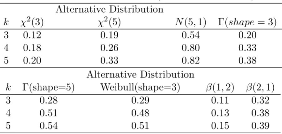
The two test statistics derived in the previous sections are too com-plicated to allow deriving their exact distributions under the null hy-pothesis analytically. The critical values of the tests are obtained by a simulation using 10,000 samples and are tabulated forα= 0.05,0.1 and k = 3,4,5 in tables 1 and 3. Since the record values for larger values of k are rare, we limited k to 5, the usual number of record values in the application, in our simulation study. Another reason for not considering values ofkin excess of 5 is that the values of cor-responding test statistics become unbounded due to rounding errors. The powers of the test forα= 0.1 and different alternatives are also tabulated in tables 2 and 4.
Table 1. Critical values for different values ofk and α (upper record values)
α
k 0.05 0.1
3 6.19 5.48
4 8.12 7.38
5 11.00 10.18
Table 2. Powers of the test (upper record values)
Alternative Distribution
k χ2(3) χ2(5) N(5,1) Γ(shape= 3) Γ(shape=5)
3 0.11 0.12 0.44 0.11 0.14
4 0.12 0.14 0.62 0.15 0.22
5 0.13 0.16 0.64 0.18 0.24
Alternative Distribution
k Weibull(shape=3) LN(0,2) β(1,2) β(2,1)
3 0.21 0.32 0.12 0.38
4 0.35 0.42 0.14 0.65
5 0.37 0.52 0.17 0.82
Table 3. Critical values for different values ofk and α (lower record values)
α
k 0.05 0.1
3 8.75 6.66
4 8.94 7.32
5 12.77 9.23
Table 4. Powers of the test (lower record values)
Alternative Distribution
k χ2(3) χ2(5) N(5,1) Γ(shape= 3)
3 0.12 0.19 0.54 0.20
4 0.18 0.26 0.80 0.33
5 0.20 0.33 0.82 0.38
Alternative Distribution
k Γ(shape=5) Weibull(shape=3) β(1,2) β(2,1)
3 0.28 0.29 0.11 0.32
4 0.51 0.48 0.13 0.38
5 0.54 0.51 0.15 0.39
Acknowledgment
The authors would like to thank the refers for their attention to the topic and useful comments and suggestions.
References
[1] Ahmad, I. A. and Lin, P. E. (1976), A nonparametric estimation of the entropy for absolutely continuous distributions. IEEE Trans. Inf. Theory,22, 372–375.
[2] Arizono, I. and Ohta, H. (1989), A test for normality based on Kullback-Leibler information. The American Statistician, 43, 20–23.
[3] Arnold, B. C., Balakrishnan, N., and Nagaraja, H. N. (1998), Records. New York: John Wiley.
[4] Dmitriev, Y. G. and Tarasenko, F. P. (1973), On the estimation of functional of the probability density and its derivatives. Theory probab. Applic.,18, 628–633.
[5] Ebrahimi, N. and Habibullah, M. (1992), Testing exponentiality based on Kullback-Leibler information. J. Royal Statist. Soc. B, 54, 739–748.
[6] Glick, N. (1978), Breaking record and breaking boards. Amer. Math. Monthly,85, 2–26.
[7] Kullback, S. (1959), Information Theory and Statistics. New York: John Wiley.
[8] Park, S. (1995), The entropy of consecutive order statistics. IEEE Trans. Inform. Theory,41, 2003–2007.
[9] Park, S. (2005), Testing exponentiality based on the Kullback-Leibler information with the type II censored data. IEEE Trans. on Rel.,54, 22–26.
[10] Shannon, C. E. (1948), A mathematical theory of communica-tions. Bell System Tech. J.,27, 379–423.
[11] Teitler, S., Rajagopal, A. K., and Ngai, K. L. (1986), Maximum entropy and reliability distributions. IEEE Trans. on Rel., 35, 391–395.
[12] Vasicek, O. (1976), A test for normality based on sample en-tropy. J. Royal Statist. Soc. B, 38, 730–737.
[13] Yousefzadeh, F. and Arghami, N. R. (2007), A piece-wise linear cdf estimator and some applications. submitted.