Solving a multi-objective mixed-model assembly line balancing and sequencing problem

Solving a multi-objective mixed-model assembly line balancing and

sequencing problem

Masoud Rabbani 1*, Mehdi Yazdanbakhsh1, Hamed Farrokhi-Asl2 1

School of Industrial Engineering, College of Engineering, University of Tehran, Tehran, Iran 2

School of Industrial Engineering, Iran University of Science & Technology, Tehran, Iran [email protected], [email protected], [email protected]

Abstract

This research addresses the mixed-model assembly line (MMAL) by considering various constraints. In MMALs, several types of products which their similarity is so high are made on an assembly line. As a consequence, it is possible to assemble and make several types of products simultaneously without spending any additional time. The proposed multi-objective model considers the balancing and sequencing problems, simultaneously. Based on the assembly problem, the various tasks of models are assigned to the workstations, while in the sequencing problem, a sequence of models for production is determined. The two meta-heuristic algorithms, namely MOPSO and NSGA-II are used to solve the developed model and different comparison metrics are applied to compare these two proposed meta-heuristics. Several test problems based on empirical data is used to illustrate the performance of our proposed model. The results show that NSGA-II outperforms the MOPSO algorithm in most metrics used in this paper. Moreover, the results indicate that our proposed model is more effective and efficient to assignment of tasks and sequencing models than manual strategy. Finally, conclusion remarks and future research are provided.

Keywords: mixed-model assembly line, sequencing; balancing, mixed-integer linear programming, meta-heuristic algorithms

1- Introduction

Today, the modern industries try to provide high quality products and enhance the satisfactory level of customers and service level in the competitive market. The just-in-time (JIT) approach as the new reputed production systems is implemented in wide range of industries (Rabbani, Siadatian, Farrokhi-Asl, and Manavizadeh 2016). The mixed-model assembly lines (MMALs) are applied as one of the wildly-used approaches in JIT systems. In the MMAL, common-based products that is called models with various in size, color, material or equipment is assembled (Rekiek and Delchambre 2006). There are two main problems namely; balancing and sequencing problems are considered in the MMAL to determine the best strategy for planning of MMAL. Assembly line balancing as a mid-term period problem allocates the

*Corresponding author

ISSN: 1735-8272, Copyright c 2017 JISE. All rights reserved

Journal of Industrial and Systems Engineering

Vol. 10, special issue on production and inventory, pp 155-170 Winter (February) 2017

various tasks of models to the workstations, while in the sequencing problem as short-term period problem, a sequence of models for production is determined. There are various studies address both problems. Thomopoulos (1967), Dar-El and Nadivi (1981), Sawik (2002) investigated these problems hierarchically. In these researches, initially the balancing models is solve to find the best strategy for assignment of task to the workstations and then based on the result of this model, the sequencing problem formulates the problem to determine the best sequence of the models. Kim et al. (2000, 2006), Miltenburg (2002), Sawik (2002), Bock et al. (2006) determined the best strategic for balancing and sequencing MMAL, simultaneously. In spite of these researches, most of them is investigated two aspects of the MMAL problem, separately. Boysen et al. (2009) provided a comprehensive review for the sequencing problem and classified them. On the other hand, Becker and Scholl (2006) and Boysen et al. (2007) reviewed and classified the studies addressing assembly line balancing problem.

Boysen et al. (2009) developed a simultaneous approach for the MMAL problem and compared the proposed approach with the hierarchical approach. Their result showed the superior performance of simultaneous approach than the hierarchical approach, especially when the assignment of tasks to the workstations does not require more expenditure such as setup costs. Hwang and Katayama (2010) proposed hierarchical models for balancing and sequencing problems. They applied a priority-based multi-chromosome GA to minimize the number of workstations as the static criterion and variance of workload as the dynamic criterion. Hyun et al. (1998), Mansouri (2005), Tavakkoli-Moghaddam and Rahimi-Vahed (2006) and O¨ zcan and Toklu (2009) proposed the multi-objective model to investigate the best assignment and sequencing in the MALL problem. Rabbani, Mousavi and Farrokhi-Asl (2016) also proposed multi objective model to balance robotic mixed model assembly lines. Bukchin and Rabinowitch (2006), Roberts and Villa (1970) and Bukchin et al. (2002) assigned the tasks to workstations in a way that the minimal workstations are equipped with flexible tools, workers and machinery. The utility work is defined as the uncompleted amount of work within the given length of workstation. The minimizing the utility works are the most important objective investigated by Kim et al. (2000), Boysen et al. (2009), Hyun et al. (1998), Tsai (1995), Tavakkoli-Moghaddam and Rahimi-Vahed (2006). The balancing and sequencing of the MMAL problem are the independently NP-hard (Gutjahr and Nemhauser 1964, Tsai 1995), so the combination of them imposes an additional level of complexity. To the best of our knowledge, this research is the first study that proposes the integrated model for balancing and sequencing with three objective functions including minimization of utility work, variation in the actual and required production capacity of the line, and the setup time. The assembly problem assigns the various tasks of models to the workstations. Meanwhile, the sequencing problem determines the sequence of models for production. The two meta-heuristic algorithms namely MOPSO and NSGA-II are applied to solve the developed model. To enhance the performance of the algorithms, parameters of the two meta-heuristics are tuned by Taguchi method. Various comparison metrics are used to compare these two proposed meta-heuristics. Several test problems based on empirical data is conducted to illustrate the performance of our proposed model.

The rest of this paper is organized as follows. Section 2 describes some characteristics of the problem and mathematical model of the problem is presented in this section. In section 3, the solution methodology is explained to tackle the proposed model and the calibration of the applied meta-heuristics are done by using a Taguchi experiment design. Section 4 presents numerical experiments and comparison of the algorithms. Finally, conclusions remarks and recommendations for future studies are provided in Section 5.

2-Problem description

According to the literature review, there are three kinds of products assembled in the line such as, single-model, mixed-model, and multi-model assembly lines. On a single-model assembly line, just one product is produced with identical workstation. Whereas, in the assembling several products in one line, the sequence of the products is the most important matter that influences the efficiency of the line. In the mixed-model assembly line, the basis of products is same and the differences between models are

optional (e.g. manual or electric, sunroof for an automobile and etc.). In this research, a cyclic production strategy represented by minimum part set (MPS) determines the sequence of models. Therefore, the greatest common divisor of demand values of planning horizon is represented as Dm (m=1, 2, ... , M), and

the MPS is defined as the vector d=(d1, d2, ... , dM) where dm=Dm/h (Kim et al. 2000). When the greatest

common divisor of demand values does not exist, the demands of models must be rounded up to the nearest number to clarify the existence of the greatest common divisor. For instance, if the demands of models are considered as 50, 37 and 40, the modified demands are considered as 50, 40 and 40 instead. Therefore, the MPS vector is presented as d=(5, 4, 4) . The multi-model assembly line is defined when the products have difference in the basis and nature. In these models, the sequence of batches of models is the most important factor, because there is considerable setup time between two consecutive batches. In this paper, both problems, i.e. balancing and sequencing problems are considered simultaneously to solve the mixed-model assembly line. There are some assumptions in this research as follows.

2-1-Assumptions

• There is no buffer space in the line;

• There is a conveyor moving within the workstations;

• The launching rate of each model is fixed;

• The speed of the conveyor is constant;

• The number of workstations is predetermined;

• All workstations are closed type;

• The uncompleted tasks are passed to the utility workers;

• The tasks of models are assigned to various workstations by considering their precedence constraints;

2-2-Mathematical model

In MMAL, minimizing the total utility work is defined as the most important objective function in the literature (Hyun et al. 1998). On the other hand, the workload smoothness (Simaria and Vilarinho 2004) and total setup cost (TavakkoliMoghaddam and Rahimi-Vahed 2006) are considered as other important objective function. The proposed models are developed by considering these objective functions. The indices, parameters and variables of the MILP model are as follows:

Notations:

Sets:

S Number of sequences s∈S

N Number of stations n∈N

M Number of models m m, ′∈M

m

O Number of tasks that belong to model m o o, ′∈Om o

Pre Set of immediate precedent tasks for task o

Parameters:

n sm

v Capacity of the station n for model m in sequence s

mo

D Assembly time of task o of model m

m

d Demand of model m in the MPS

λ Rate of producing each model in required capacity

n

L Fixed line length of station n

mm n

n

v Speed of the conveyor in station n including the main line and sub-line

γ

Variables: sn

U Amount of the utility work required for performing the assigned tasks to station n at sequence s

n

EP Ending position of operator for last model in the station n

sn

SP Starting positions of the work sequence s in station n

n mm s

X ′ Binary variable, it is 1 if model types m and m’ are assigned sequentially at station n; otherwise, 0

n mos

Y Binary variable, it is 1 if task o of model m at sequence s is assigned to station n, otherwise 0 Mathematical formulation:

1

min ( _{sn n})

n N s S

z U EP

∈ ∈

=

∑ ∑

2

min ( )

m

n n

mos sm m

n N s S m M o O

z Y v

λ

∈ ∈ ∈ ∈

=

∑ ∑ ∑ ∑

3

min _{mm s}n

n

mm n N s S m M m M

z X _′t

′

∈ ∈ ∈ ∈ ′

=

∑ ∑ ∑ ∑

s.t.

1 1

n m s n N m M

Y

∈ ∈

=

∑ ∑

1

n

m s m

n N s S

Y d

∈ ∈

=

∑ ∑

, 1,

n n

mo s m o s

n N n N

nY _′ nY ₊

∈ = ∈

∑

∑

( )

m

n

sn mo mos n sn n

m M o O

SP D Y v U L

∈ ∈

+

∑ ∑

1,

( )

m

n

sn mo mos n sn n s n

m M o O

SP D Y v U

γ

∈ ∈

+

∑ ∑

( )

m

n

Sn mo moS n Sn n n

m M o O

SP D Y v U

γ

∈ ∈

+

∑ ∑

, 1 1

2

n n

mos m o s n

mm s

Y Y

X

′ ′ +

′

+ − _{≤ , , , , , , 1,..., 1}

m m

m m′ M m m o′ O o′ O _′ n N s S

∀ ∈ ≠ ∈ ∈ ∈ = − (10)

, 0

sn sn

U SP ≥ ∀ ∈n N s, ∈S (11)

0

n

EP ≥ ∀ ∈n N (12)

{0,1}

n mm s

X _′ = ∀m m, ′∈M m, ≠m o′, ∈O_m,o′∈O_m′,n∈N s, =1,...,S −1 (13)

{0,1}

n mos

Y = ∀ ∈m M o, ∈Om,n∈N s, ∈S (14)

Equation (1) is the objective function of the model in order to minimize the total utility work and the ending position of each operator in each station. Equation (2) calculates the variation in the actual and required production capacity of the line. Equation (3) calculates the total setup time and aims to minimize it. Constraint (4) enforces that in each sequence exactly one model must be completed. Constraint (5) emphasizes that the demand of each model in the MPS must be satisfied. Precedence constraints are considered in Constraint (6).Constraint (7) calculates the utility work required for each sequence at each station. Constraints (8) and (9) are pertaining to the starting position of the operator after finishing each model and the ending position of the operator, respectively. The sequencing of the models are determined by Constraint (10). Constraints (11) and (12) indicate that the positive variables. Also, Constraints (13) and (14) represent the range of the variables.

3- Solution Methodology

In this section, we present two solution approaches including two multi-objective evolutionary algorithms; that is, non-dominated sorting genetic algorithm (NSGA-II) and multi-objective particle swarm optimization (MOPSO).

3-1-Solution representation

We design chromosomes or particles to present each solution. In this research, the continuous solution representations are considered as chromosomes. The first chromosome contain some genes that is equal to sum of the elements of MPS vector with random numbers in the range of e [0, 1]. The models are sequenced based on the value of corresponding genes in the chromosome from large to small as shown in Figure 1. This chromosome represents the permutation of models based on the MPS vector. For example, consider the MPS vector as d=(2, 1, 2). Figure 1 represents this chromosome as follow:

models

1 2 3 4 5

Sequence of models

0.89 0.27 0.79 0.75 0.95

Fig 1. The illustrative example for the first Chromosome

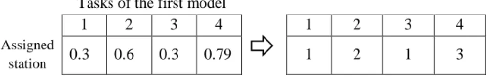
The second chromosome represents the assigning of the operation of the models to the stations. The number of the components in the second chromosome is equal to the number of the models (five in the previous example). Each component has some genes which is equal to number of the tasks of corresponding model with random numbers in the range of [0, 1]. Then, all genes of the components are multiplied by the number of stations and then rounded up. For example, if the number of task for the first model is equal to the four and the number of the station is three, the representation of the second chromosome is as follows:

Tasks of the first model

1 2 3 4 1 2 3 4

Assigned

station 0.3 0.6 0.3 0.79 1 2 1 3

Fig 2. The structure of the first component of the second chromosome

3-2- NSGA-II

Genetic Algorithm (GA) was developed by John Holland, which is inspired from inheriting the characteristics of species. Because of being a population based methodology, the GA approach is appropriate for solving the multi-objective optimization problems (Rabbani, Farrokhi-Asl and Ameli 2016). Indian scholars Srinivas and Deb (1994) proposed a Non-dominated Sorting Genetic Algorithm (NSGA). Focusing on population classification layer by layer is the NSGA approach to solve the problem. Prior to the operation of selection, sort the non-inferiority of all individuals of the population, represent the value of their non-dominated sorting and allot larger value to superior individuals so that they can be inherited with higher probability. To keep up the population differences the sharing function and niche technology are additionally embraced. The optimal solutions are distributed evenly that are advantages of NSGA. The computational efficiency is not good enough and the imparting parameter is artificially set as the elitist strategy is not received in the algorithm, these are the impediments of this algorithm. Deb et al. (2000) altered NSGA and proposed NSGA-II to make up for the shortcomings of NSGA. To lessen the computational complexity the algorithm adopts fast sorting of the non-inferiority of all individuals and to abstain setting the imparting parameter artificially uses congestion. What’s more, it adopts elite strategy to make superior individuals in parent generation compete with superior ones in filial generation, thus, the new generation could be more superior. Several researches have demonstrated that NSGA-II with elitist strategy has the ability of getting evenly distributed Pareto optimal, and it has indicated strong advantage in multi-objective optimization area.

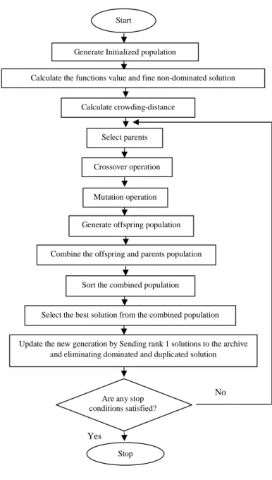
Fig 3. The flow chart of the NSGA-II

3-2-1-Crossover and mutation operators

For doing crossover operator, two individuals are selected randomly from the populations. We select two genes from selected chromosome and we change the place of these genes with each other. For the second chromosome, two selected individuals from the populations replace the assignment of the same models with each other to generate offspring.

For mutation operator, an individual will be selected randomly. We choose two genes of the chromosome randomly and change the place these genes with each other. For the second chromosome, we chose one gene randomly. Then, one model is selected and the new assignment for its operation is done.

No Calculate the functions value and fine non-dominated solution

Calculate crowding-distance

Select parents

Crossover operation

Mutation operation

Generate offspring population

Stop Start

Generate Initialized population

Combine the offspring and parents population

Sort the combined population

Select the best solution from the combined population

Update the new generation by Sending rank 1 solutions to the archive and eliminating dominated and duplicated solution

Are any stop conditions satisfied?

3-3- MOPSO

The essential goal of each multi-objective optimization method is to find not only one, however a set of rational solutions, called Pareto optimal set. In other words, the fundamental aim is to recognize an exact Pareto optimal set of answers that are globally non-dominated and are well-distributed along the Pareto front (Rabbani, Farrokhi-Asl et al. 2016). The idea of domination and Pareto optimality are totally cleared up in the literature. Particle swarm optimization is a meta-heuristic strategy which is inspired by the developments of a group of feathered creatures or fishes who look for food. This technique is a prominent optimization approach due to its relative straightforwardness in contrast with other evolutionary algorithms and is a suitable applying for multi-objective optimization issues. Notwithstanding the way that no improvement technique is suitable for different sorts of problems that could promise discovering the ideal solution, MOPSO has showed a superior execution contrasted with other evolutionary multi-objective optimization algorithms in the literature of this field (Rabbani, Mousavi et al. 2016). Hence, this fact motivates us to utilize MOPSO as a part of this study to improve the objectives defined. Moore and Chapman (1999) were the first persons who proposed MOPSO in an unpublished composition.

The MOPSO utilized as a part of this article is a predominance based technique proposed by Coello et al (2004). In this method, the best non-dominated solutions that have ever been found by algorithm are put away in a repository. Speed and position of every particle are figured through the accompanying following relations:

1

1 1 2 2

t t t t t t

i i i i h i

v+ =wv +c R p_ −x _+c R rep_ −x _ (15)

1 1

t t t

i i i

x + = x +v + (16)

Where represents the current velocity of i-th particle and shows the current position of i-th particle. R1 and R2 are uniform random numbers between [0, 1]. A personal learning coefficient is shown

as c1 and c2 represents a global learning coefficient. Inertia weight is considered as w. Also, is the best

experience of the i-th particle and the best nominated repository member that are chosen by roulette wheel selection method is indicated as . The general structure of the MOPSO is represented as fallow:

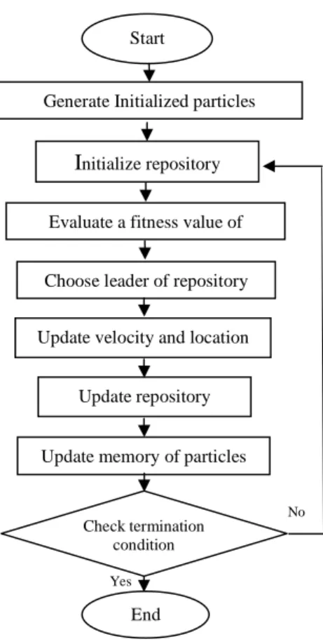
Fig 4. The flow chart of the MOPSO

3-4- Parameter tuning

NSGA-II parameters that we tune consist of number of solution in the initial population (npop), crossover rate (pc) and mutation parameters (pm). To outline of the experiment, we utilize Taguchi method. The experiment’s factors are npop, pc, and pm. We consider 4 levels for each factor and use Minitab software to design experiment and analyze its result. We solve the medium-size problem according to the design of experiment method named Taguchi method for tuning parameters. The consequences of experiments and analyzing about parameters are shown as follow:

Initialize repository Evaluate a fitness value of

Choose leader of repository Update velocity and location

Update repository

Update memory of particles

Check termination condition

End

Start

Generate Initialized particles

No

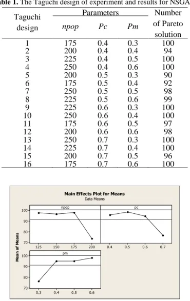
Table 1. The Taguchi design of experiment and results for NSGA-II

Taguchi design

Parameters Number

of Pareto solution

npop Pc Pm

1 175 0.4 0.3 100

2 200 0.4 0.4 94

3 225 0.4 0.5 100

4 250 0.4 0.6 100

5 200 0.5 0.3 90

6 175 0.5 0.4 92

7 250 0.5 0.5 98

8 225 0.5 0.6 99

9 225 0.6 0.3 100

10 250 0.6 0.4 100

11 175 0.6 0.5 97

12 200 0.6 0.6 98

13 250 0.7 0.3 100

14 225 0.7 0.4 100

15 200 0.7 0.5 96

16 175 0.7 0.6 100

200 175 150 125 100 90 80 70 0.7 0.6 0.5 0.4 0.6 0.5 0.4 0.3 100 90 80 70 npop M e a n o f M e a n s pc pm

Main Effects Plot for Means

Data Means

Fig 5. The analysis of Taguchi design for NSGA-II parameters

We can understand which amount of parameter is suitable and has a better result from analyzing Diagrams. Abstract of diagrams and results are summarized in Table 2.

Table 2. The result of parameters tuning for NSGA-II

Parameter npop Pc Pm

Best value 175 0.4 0.6

MOPSO parameters that we tune consist of personal learning coefficient (c1), global learning coefficient

(c2), Inertia weight (w), Repository size (nRep), and damping rate for inertia weight (wdep). We utilize

Taguchi method to outline of the experiment. We consider four levels for each factor and use Minitab software to design experiment and analyze its result. For tuning parameters we solve the medium-size problem according to the design of experiment method called Taguchi method. The consequences of experiments and analyzing about parameters are shown in Table 3.

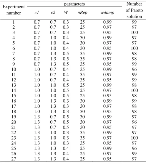
Table 3. The Taguchi design of experiment and results for MOPSO

Experiment number

parameters Number

of Pareto solution

c1 c2 W nRep wdamp

1 0.7 0.7 0.3 25 0.99 99

2 0.7 0.7 0.3 25 0.97 97

3 0.7 0.7 0.3 25 0.95 100

4 0.7 1.0 0.4 30 0.99 97

5 0.7 1.0 0.4 30 0.97 97

6 0.7 1.0 0.4 30 0.95 100

7 0.7 1.3 0.5 35 0.99 98

8 0.7 1.3 0.5 35 0.97 98

9 0.7 1.3 0.5 35 0.95 99

10 1.0 0.7 0.4 35 0.99 96

11 1.0 0.7 0.4 35 0.97 99

12 1.0 0.7 0.4 35 0.95 99

13 1.0 1.0 0.5 25 0.99 98

14 1.0 1.0 0.5 25 0.97 100

15 1.0 1.0 0.5 25 0.95 98

16 1.0 1.3 0.3 30 0.99 99

17 1.0 1.3 0.3 30 0.97 98

18 1.0 1.3 0.3 30 0.95 98

19 1.3 0.7 0.5 30 0.99 97

20 1.3 0.7 0.5 30 0.97 96

21 1.3 0.7 0.5 30 0.95 97

22 1.3 1.0 0.3 35 0.99 97

23 1.3 1.0 0.3 35 0.97 100

24 1.3 1.0 0.3 35 0.95 97

25 1.3 1.3 0.4 25 0.99 96

26 1.3 1.3 0.4 25 0.97 99

27 1.3 1.3 0.4 25 0.95 97

1.3 1.0 0.7 26 24 22 20 1.3 1.0

0.7 0.3 0.4 0.5

35 30 25 26 24 22 20 0.99 0.97 0.95 c1 M e a n o f M e a n s c2 w nrep wdep

Main Effects Plot for Means

Data Means

Fig 6. The analysis of Taguchi design for MOPSO parameters

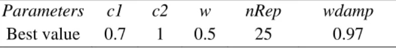
We can understand which amount of parameter is suitable and has a better result from analyzing Diagrams. Abstract of diagrams and results are summarized in Table 4.

Table 4. The results of parameters tuning for MOPSO

Parameters c1 c2 w nRep wdamp

Best value 0.7 1 0.5 25 0.97

4- Numerical results

As it is explained, tuned NSGA-II and MOPSO algorithms are applied to tackle the proposed mathematical model. These calculations actualized on an Intel Core i3 2.67 GHz PC with 2GB RAM and have been coded in MATLAB R2014a to validate the execution of these two algorithm. The performance metrics used for evaluating multi-objective algorithms are different from criteria used to evaluate single-objective algorithms. In this paper, some qualitative and quantitative metrics are used to tune the parameters, assess and compare the performance of MOPSO and NSGA-II (Asefi et al. 2014; Karimi, Zandieh, and Karamooz, 2010; Behnamian, Ghomi, and Zandieh, 2009).

Number of Pareto solutions (NPS):

This performance metric is introduced as the quantity of non-dominated solutions that each algorithm can obtain. Larger number of Pareto solutions results in better performance.

Spread of non-dominated solutions:

This criterion is known as an indicator diversity. Larger values of this metric represent higher quality of solutions. This metric is computed by:

( )

1 i i n

MID c SNS

n ∈

− =

−

∑

(17)

where n is the number of non-dominated solution, and MID shows the mean distance from ideal point. Since all objective functions in this paper are minimization, the origin point is considered as an ideal point. ci denotes the distance between i solution from ideal point.

Diversification matrix (DM): The diversity of solutions that each algorithm can obtain is calculated by

this performance criterion. The value of this criterion is calculated by:

2 2 2

1 1 2 2 3 3

(max _i min _i) (max _i min _i) (max _i min _i)

DM = f − f + f − f + f − f (18)

Mean ideal distance (MID): The value of this criterion indicates the closeness between the ideal point

and Pareto solutions. The lower value represents the best performance of the algorithm.

i i n

c M ID

n

∈

=

∑

2 2 2

1 2 3

i i i i

c

=

f

+

f

+

f

∀ ∈

i

n

where denotes the value of i-th objective for solution j.

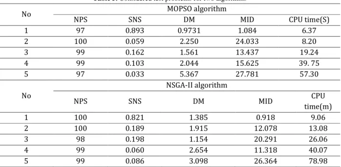
Each test problem is solved for five times and the averages of these results are reported in Table 5. Due to illustrate the performance of these algorithms, NSGA-II and MOPSO are implemented in various size problems. We compare this two algorithm in terms of a number of Pareto solutions (NPS), diversification metric (DM), spread of non-dominance solutions (SNS), mean ideal distance (MID) and computational

time. According to the results obtained from all test problems, the comparison of metrics and results is illustrated in Table 5.

Table 5. Considered test problems for two algorithms

No MOPSO algorithm

NPS SNS DM MID CPU time(S)

1 97 0.893 0.9731 1.084 6.37

2 100 0.059 2.250 24.033 8.20

3 99 0.162 1.561 13.437 19.24

4 99 0.103 2.044 15.625 39. 75

5 97 0.033 5.367 27.781 57.30

No

NSGA-II algorithm

NPS SNS DM MID CPU

time(m)

1 100 0.821 1.385 0.918 9.06

2 100 0.189 1.915 12.078 13.08

3 98 0.198 1.154 20.291 26.06

4 99 0.060 2.654 11.318 40.07

5 99 0.086 3.098 26.364 78.98

The results can be summarized as follows:

1. MOPSO can obtain better results in terms of the computational time than NSGA-II. NSGA-II can search more solution space than MOPSO, so this higher running time is logical.

2. NSGA-II can achieve a greater number of Pareto-solutions (NPS) than MOPSO.

3. The average value of the diversification metric (DM) for NSGA-II is less than MOPSO. However, it is not much difference between these algorithms and do not prefer one over another from the perspective of the DM.

4. Based on the spread of non-dominance solutions (SNS) in NSGA-II indicates the superiority than the SNS in MOPSO. Since the larger value of this metric represents the highest quality of the solution, the quality of the solutions in NSGA-II is better than the quality of solutions in MOPSO.

5. The closeness between the ideal point and Pareto solutions represents the mean ideal distance (MID). According to the results, NSGA-II represents a better performance than MOPSO because of the low value of the MID.

Generally, NSGA-II almost in all factors of the test problem has a better performance than MOPSO. We can find out from Tables 5 that NSGA-II outperforms MOPSO in planning and scheduling, especially in problems considered in this paper.

5-Conclusion

In this research, the mixed-model assembly line (MMAL) was investigated. Two most important challenges in the MMAL problem are the balancing and sequencing products in the assembly line. We proposed integrated model to balance and sequence the products, simultaneously. Based on the assembly problem, the various tasks of models were assigned to the workstations, while in the sequencing problem, a sequence of models for production was determined. To solve the proposed model, the MOPSO and NSGA-II algorithms were developed. The Taguchi method was applied to enhance the performance of the proposed algorithms by tuning their parameters. Several test problems based on historical data were used to show the performance of our proposed model. The results showed that NSGA-II outperforms the

MOPSO algorithm in most metrics used in this paper. Based on the results, our proposed model is more effective and efficient to assignment of tasks and sequencing models than manual strategy. We suggest to interested readers in this field to formulate the problem based on other uncertain approach such as, stochastic programming approach, robust approach, and fuzzy-stochastic approach. Appling the other exact solution methodologies to solve the proposed model in the future researches can be interesting challenge. As another proposed research area, the game theory can be used to formulate the problem.

Reference

Asefi, H., F. Jolai, M. Rabiee, and M. T. Araghi. 2014. “A hybrid NSGA-II and VNS for solving a bi-objective no-wait flexible flowshop scheduling problem.” The International Journal of Advanced Manufacturing Technology 75: 1017-1033.

Becker, C. and Scholl, A., 2006. A survey on problems and methods in generalized assembly line balancing. European Journal of Operational Research, 168 (3), 694–715.

Behnamian, J., S. F. Ghomi, and M. Zandieh. 2009. “A multi-phase covering Pareto-optimal front method to multi-objective scheduling in a realistic hybrid flowshop using a hybrid metaheuristic.” Expert Systems with Applications 36: 11057-11069.

Bock, S., Rosenberg, O., and Brackel, T.V., 2006. Controlling mixed-model assembly lines in real-time by using distributed systems. European Journal of Operational Research, 168 (3), 880–904.

Boysen, N., Fliedner, M., and Scholl, A., 2007. A classification of assembly line balancing problems. European Journal of Operational Research, 183 (2), 674–693.

Boysen, N., Fliedner, M., and Scholl, A., 2009. Sequencing mixed-model assembly lines: survey, classification and model critique. European Journal of Operational Research, 192 (2), 349–373.

Bukchin, J., Dar-El, E.M., and Rubinovitz, J., 2002. Mixed model assembly line design in a make-to-order environment. Computers & Industrial Engineering, 41 (4), 405–421.

Bukchin, Y. and Rabinowitch, I., 2006. A branch-and-bound based solution approach for the mixed-model assembly linebalancing problem for minimizing stations and task duplication costs. European Journal of Operational Research, 174 (1), 492–508. International Journal of Production Research 5013 Cochran, W.G. and Cox, G.M., 1992. Experimental designs. 2nd ed. New York: Wiley.

Coello, C. A. C, Pulido, G. T, & Lechuga, M. S. handling multiple objectives with particle swarm optimization. Evolutionary Computation, IEEE Transactions on, 8(3), 256-279 (2004)

Dar-El, E.M. and Nadivi, A., 1981. A mixed–model sequencing application. International Journal of Production Research, 19 (1), 69–84.

Deb K, Pratap A, Agarwal S, and Meyarivan T. A. M. T, A fast and elitist multi-objective genetic algorithm: NSGA-II, IEEE Transactions on Evolutionary Computation, 6, 182-197 (2002)

Deb, K., Agrawal, S., Pratap, A., & Meyarivan, T. (2000). A fast elitist non-dominated sorting genetic algorithm for multi-objective optimization: NSGA-II. Lecture notes in computer science, 1917, 849-858. Erel, E., Gocgun, Y., and Sabuncuog˘ lu, _I., 2007. Mixed-model assembly line sequencing using beam search. International Journal of Production Research, 45 (22), 5265 – 5284.

Gutjahr, A.L. and Nemhauser, G.L., 1964. An algorithm for the line balancing problem. Management Science, 11 (2), 308–315.

Holland, J, Adaptation in Natural and Artificial Systems. Ann Harbor: University of Michigan (1975) Hwang, R. and Katayama, H., 2010. Integrated procedure of balancing and sequencing for mixed-model assembly lines: a multiobjective evolutionary approach. International Journal of Production Research, 48 (21), 6417 – 6441.

Hyun, C.J., Kim, Y., and Kim, Y.K., 1998. A genetic algorithm for multiple objective sequencing problems in mixed model assembly lines. Computers & Operations Research, 25 (7–8), 675–690.

Karimi, N., M. Zandieh, and H. R. Karamooz. 2010. “Bi-objective group scheduling in hybrid flexible flow shop: A multi-phase approach.” Expert Systems with Applications 37: 4024-4032.

Kim, Y.K., Hyun, C.J, and Kim, Y., 1996. Sequencing in mixed model assembly lines: a genetic algorithm approach. Computers & Operations Research, 23 (12), 1131–1145.

Kim, Y.K., Kim, J.Y., and Kim, Y., 2000. A coevolutionary algorithm for balancing and sequencing in mixed model assembly lines. Applied Intelligence, 13 (3), 247–258.

Kim, Y.K., Kim, J.Y., and Kim, Y., 2006. An endosymbiotic evolutionary algorithm for the integration of balancing and sequencing in mixed-model u-lines. European Journal of Operational Research, 168 (3), 838–852.

Mansouri, S.A., 2005. A multi-objective genetic algorithm for mixed-model sequencing on JIT assembly lines. European Journal of Operational Research, 167 (3), 696–716.

Miltenburg, J., 2002. Balancing and scheduling mixed-model u-shaped production lines. International Journal of Flexible Manufacturing Systems, 14 (2), 119–151.

Montgomery, D.C., 2000. Design and analysis of experiments. 5th ed. New York: Wiley.

Moore J, Chapman R, Application of particle swarm to multiobjective optimization. Department of Computer Science and Software Engineering, Auburn University (1999)

Naderi, B., Zandieh, M., and Fatemi Ghomi, S.M.T., 2009. Scheduling job shop problems with sequence-dependent setup times. International Journal of Production Research, 47 (21), 5959 – 5976.

Rabbani, M., Farrokhi-Asl, H., & Ameli, M. (2016). Solving a fuzzy multi-objective products and time planning using hybrid meta-heuristic algorithm: Gas refinery case study. Uncertain Supply Chain Management, 4(2), 93-106.

Rabbani, M., Mousavi, Z., & Farrokhi-Asl, H. (2016). Multi-objective metaheuristics for solving a type II robotic mixed-model assembly line balancing problem. Journal of Industrial and Production Engineering, 1-13.

Rabbani, M., Siadatian, R., Farrokhi-Asl, H., & Manavizadeh, N. (2016). Multi-objective optimization algorithms for mixed model assembly line balancing problem with parallel workstations. Cogent Engineering, (just-accepted), 1158903.

Rekiek, B. and Delchambre, A., 2006. Assembly line design: the balancing of mixed-model hybrid assembly lines with genetic algorithms. 1st ed. London: Springer.

Roberts, S.D. and Villa, C.D., 1970. On a multiproduct assembly line-balancing problem. AIIE Transactions, 2 (4), 361–364.

Sawik, T., 2002. Monolithic vs. hierarchical balancing and scheduling of a flexible assembly line. European Journal of Operational Research, 143 (1), 115–124.

Scholl, A., 2010. Homepage for assembly line optimization research. Available from:5http://www.assembly–line–balancing.de/4 [Accessed 10 July 2010].

Simaria, A.S. and Vilarinho, P.M., 2004. A genetic algorithm based approach to the mixed-model assembly line balancing problem of type ii. Computers & Industrial Engineering, 47 (4), 391–407.

Srinivas, N., & Deb, K. (1994). Muiltiobjective optimization using nondominated sorting in genetic algorithms. Evolutionary computation, 2(3), 221-248.

Taguchi, G., 1986. Introduction to quality engineering: designing quality into products and processes. 1st ed. White Plains, NY: Asian Productivity Organization.

Tavakkoli-Moghaddam, R. and Rahimi-Vahed, A.R., 2006. Multi-criteria sequencing problem for a mixed-model assembly line in a JIT production system. Applied Mathematics and Computation, 181 (2), 1471–1481.

Thomopoulos, N.T., 1967. Line balancing-sequencing for mixed-model assembly. Management Science, 14 (2), 59–75.

Tsai, L.H., 1995. Mixed-model sequencing to minimize utility work and the risk of conveyor stoppage. Management Science, 41 (3), 485–495.